NBER WORKING PAPER SERIES
COINTEGRATION AND CONSUMPTION RISKS IN ASSET RETURNS Ravi Bansal
Robert Dittmar Dana Kiku Working Paper 13108
http://www.nber.org/papers/w13108
NATIONAL BUREAU OF ECONOMIC RESEARCH 1050 Massachusetts Avenue
Cambridge, MA 02138 May 2007
An earlier draft of this paper was circulated with the title "Long Run Risks and Equity Returns." We would like to thank George Tauchen, Jessica Wachter, Vivian Wang, Amir Yaron, and the seminar participants at Arizona State University, Duke University, Simon Fraser University, Stanford University, University of British Columbia, University of Michigan, University of North Carolina, University of Pennsylvania, Vanderbilt University, Federal Reserve Board of Governors Conference on Risk Premiums: Time Variation and Macroeconomic Links, and 2007 American Finance Association Meetings for helpful comments. The views expressed herein are those of the author(s) and do not necessarily reflect the views of the National Bureau of Economic Research.
© 2007 by Ravi Bansal, Robert Dittmar, and Dana Kiku. All rights reserved. Short sections of text, not to exceed two paragraphs, may be quoted without explicit permission provided that full credit,
Cointegration and Consumption Risks in Asset Returns Ravi Bansal, Robert Dittmar, and Dana Kiku
NBER Working Paper No. 13108 May 2007
JEL No. C01,C13,G00,G1,G12
ABSTRACT
We argue that the cointegrating relation between dividends and consumption, a measure of long run consumption risks, is a key determinant of risk premia at all investment horizons. As the investment horizon increases, transitory risks disappear, and the asset's beta is dominated by long run consumption risks. We show that the return betas, derived from the cointegration-based VAR (EC-VAR) model, successfully account for the crosssectional variation in equity returns at both short and long horizons; this is not the case when the cointegrating restriction is ignored. Our evidence highlights the importance of cointegration-based long run consumption risks for financial markets.
Ravi Bansal
Fuqua School of Business Duke University 1 Towerview Drive Durham, NC 27708 and NBER [email protected] Robert Dittmar
Stephen M. Ross School of Business University of Michigan 701 Tappan Street Ann Arbor, MI 48109 [email protected] Dana Kiku Finance Department Wharton School University of Pennsylvania 3620 Locust Walk Philadelphia, PA 19104-6367 [email protected]
Introduction
How does the riskiness of equity returns change with investment horizon? We show that at long horizons risks are dominated by long run consumption risks in dividends, while at short horizons, additional price risks may also matter. The cointegrating relation between dividends and consumption measures long-run covariance consumption risks in dividends. We show that this cointegrating relation has important conceptual and empirical implications for the risks at all horizons. Empirically, we document that consumption asset betas determined by the cointegration based vector-autoregression (EC-VAR) can very well account for the mean equity returns in the cross-section at both short and long horizons. This is not the case when the cointegration restriction, as is traditionally done, is ignored. Hence, our evidence underscores the economic importance of the cointegrating relation in understanding sources of risks and explaining equity risk premia across all investment horizons.
Our focus on the cointegrating relation is motivated by Bansal and Yaron (2004), Bansal, Dittmar, and Lundblad (2001, 2005), Hansen, Heaton, and Li (2005), and Bansal, Gallant, and Tauchen (2005) who show that long run risks can be important in explaining risk premia. Cointegration, as made clear by the representation theorem of Granger and Engle (1987), has sharp implications for predictability. In the context of dividends and consumption, the representation theorem implies that the deviation of the level of dividends from consumption (the error-correction variable) is important for predicting dividend growth rates and returns at all horizons. As the error-correction variable alters the information set used to predict future returns, it also significantly influences the return innovation and, hence, the conditional consumption betas.
The empirical literature frequently imposes the implicit assumption of no cointegration by modeling returns with a standard vector autoregression (VAR). We show that this traditional approach leads to a significant deterioration in the ability of consumption-based models to
explain risk premia at both short and long horizons relative the the cointegration-based specification. In this “standard VAR”, consumption and dividend growth rates are stationary, however the levels of consumption and dividends are not cointegrated. Deviations of dividends from consumption contain a unit root and, thus, the two series can drift far apart — there is no error-correction mechanism, which ties dividends and consumption together in the long run. Cointegration, and the implied EC-VAR framework, ties these two series together in the long run; for this reason, the error-correction term can be quite important for predicting future returns and growth rates. The inclusion of the error-correcting mechanism can significantly alter the transition dynamics of returns and asset betas relative to the standard growth-rate based VAR specification.
We first document that the error-correction term in the dividend-consumption cointegrating relation contains important information for predicting future dividend growth and returns. Imposing cointegration, we are able to predict on average 11.5% of the variation in one-year returns, compared to 7.5% when we do not impose cointegration. This difference is even starker at longer horizons: at the 10-year horizon, the EC-VAR specification results in an average 44.0% adjusted R2, compared to 9.9% for the standard growth-rate VAR specification. That is, at longer horizons, we are able to predict far more variation in returns using the cointegration specification than when we do not impose cointegration on the return dynamics. This predictability evidence suggests that cointegration has important implications for measuring return innovations and, consequently, conditional consumption betas.
Using the EC-VAR, we find that the cointegrating relation indeed significantly influences the conditional consumption betas and resulting prices of risk at all investment horizons. The estimated market price of consumption risks is always positive and significant. For example, at the short horizon, the market price of risk is 1.19 (SE=0.41); at the long horizon, it continues to be highly significant of 0.72 (SE=0.25). Our conditional consumption betas account for about 75% of the cross-sectional variation in risk premia at the one-year horizon, and are able
to explain over 85% of the the cross-section of mean returns at long horizons. In contrast, VAR models traditionally used in the literature ignore the cointegrating relation in measuring conditional betas and, hence, are unable to account for the differences in risk premia across assets. The unconditional consumption CAPM also fails to explain the variation in average returns across assets. To confirm our findings we conduct a series of Monte Carlo experiments and show that our empirical evidence is statistically significant and robust.
The unique dimension of our paper is to show that after accounting for the long-run relation between dividends and consumption, conditional consumption betas contain important information about risk premia at all investment horizons. At long horizons, transitory risks vanish and only long-run risks drive risk compensations. Our approach, therefore, allows us to analyze the size of the compensation for long-run versus transitory risks in accounting for risk premia. Quantitatively, we find that long-run consumption risks are the dominant source of risk premia at all investment horizons. Conceptually, we provide a framework for linking the cointegration parameter to the conditional consumption betas by horizon and show that they can explain the cross-sectional variation in expected returns at both short and long horizons. Earlier work has pursued a very different approach to account for the cross-sectional variation in short-horizon (one period) returns. In particular, Bansal, Dittmar, and Lundblad (2001, 2005) and Hansen, Heaton, and Li (2005) focus on cash-flow betas and inquire if these betas can account for short horizon expected returns. Parker and Julliard (2005) measures covariance risk between current returns and future consumption, while Lettau and Ludvigson (2001) and Jagannathan and Wang (1996) rely on time-varying betas to justify the cross-sectional pattern in one period expected returns.
A rich array of specifications for dividends have been used in earlier asset pricing models. In Campbell and Cochrane (1999), and Bansal and Yaron (2004) models, consumption and dividend growth rates have the same unconditional mean but are not cointegrated. Cochrane,
of aggregate dividends differ across sectors and analyze the implications for risk premia. Menzly, Santos, and Veronesi (2004) consider a specification where dividends and consumption across all sectors have unit cointegration, while Bansal, Dittmar, and Lundblad (2001) and Hansen, Heaton, and Li (2005) entertain specifications that permit heterogeneity in the cointegrating relation between dividends and consumption. The economic implications of these alternative specifications of dividends for the risk-return relation are empirically evaluated in this paper. As stated above, the heterogeneity in the cointegrating relation is found to be empirically important for understanding risk premia across assets at all investment horizons. Specifications which do not allow for this heterogeneity are not supported in the data. The empirical evidence in this paper, therefore, suggests that developing dynamic models that permit heterogeneity in the cointegrating relation would be very valuable.
The rest of the paper is organized as follows. In Section 1, we discuss a brief and simple theoretical framework and present our econometric specification for return dynamics. Section 2 describes the data. Section 3 contains the results of our empirical analysis. Monte Carlo evidence that supports our data findings is discussed in Section 4. Finally, Section 5 provides concluding remarks.
1
Cointegration and Risk Premia
In this section, we discuss a simple theoretical framework that we employ and implications of cointegration for risk measures and risk premia. Throughout our discussion, we utilize a Taylor series approximation for log returns (see Campbell and Shiller (1988)). Let zt=pt−dt represent the log of the price-dividend ratio. The return approximation is given by
where the log-linearization constantsκ0 and κ1 are,
κ1 = exp(¯z)
1 + exp(¯z), (2)
κ0 = log(1 + exp(¯z))−κ1z,¯
and ¯z is the mean of the log price-dividend ratio. Using ∆zt+s = zt+s−zt, equation (1) also implies
rt+1 =κ0 + ∆dt+1+ ∆zt+1+ (κ1−1)zt+1. (3)
We further assume that the log price-dividend ratio, zt, and dividend growth rates, ∆dt+1, are covariance stationary processes. To model long-horizon returns, it is useful to define the summed level of the price-dividend ratio as zt+1→t+s ≡ sj=1zt+j, the accumulated change in it as ∆zt+1→t+s ≡ zt+1→t+s−zt→t+s−1, and accumulated s-period growth rate as ∆dt+1→t+s ≡
s
j=1∆dt+j. Using the return expression (3), it follows that s-horizon compounded return,
rt+1→t+s ≡
s
j=1rt+j, is completely characterized by these three components.
1.1
Risk Premia
We assume, as in Lucas (1978), that a representative agent prices assets across various investment horizons. The Euler equation associated with this agent will therefore determine the risk-return relation at all horizons. To keep the analysis simple, we further assume that the representative agent’s preferences are characterized by the standard power utility of aggregate consumption. Hence, the log of the one-step-ahead stochastic discount factor is mt = ln()−γ∆ct, where ∆ct is the growth rate of log aggregate consumption, γ is the parameter of risk aversion, and determines time preferences. The standard asset pricing
condition for any horizons is,
Et[exp(mt+1→t+s+rt+1→t+s)] = 1, (4)
wheremt+1→t+s =sj=1mt+j. We assume that the log of the stochastic discount factor and log returns are jointly conditionally normal and homoskedastic, and ∆ct is a covariance stationary process. Our preference and distributional assumptions are similar to those used by Hansen and Singleton (1983).1
Let ηt+1 ≡ ∆ct+1 −Et[∆ct+1] be the one-step ahead innovation in consumption growth and ηt+1→t+s be the innovation in the cumulative growth in consumption, ∆ct+1→t+s. The conditional variance of the cumulative consumption growth corresponds to the variance of this
s-period innovation, which we denote asσc,s2 . Similarly,ηr,t+1→t+s is the innovation ins-horizon return,rt+1→t+s,σr,s2 denotes its conditional variance, andCov[ηt+1→t+s, ηr,t+1→t+s] corresponds to the conditional covariance between consumption and return innovations for horizon s. Given our distributional assumption of homoscedasticity, all conditional second moments are constants. The asset pricing condition in eq.(4) along with distributional assumptions implies that the conditional expected return at any horizon s is given by,
1 sEt rt+1→t+s+ 0.5σ2r,s−srt,sf = 1 s γ Cov[ηt+1→t+s, ηr,t+1→t+s] = 1 s γ σ 2 c,s Cov[ηt+1→t+s, ηr,t+1→t+s] σc,s2 (5) = λs βs,
where rft,s is the yield on an s-period discount bond known at date t. λs ≡ 1
s γ σ 2
c,s is
1It is straightforward to extend the presented framework to a more general framework such as in Bansal and Yaron (2004). This, however, would entail estimation of a larger set of parameters in the cross-section of assets. To avoid this, we confine our attention to the case of power utility, which is sufficient for addressing questions about the cross-sectional dispersion in mean returns that are the focus of this paper.
the price of risk that is determined by the agent’s risk aversion and the conditional variance of consumption growth for the corresponding investment horizon, and βs is the conditional consumption risk measure for horizon s. We scale expression (5) by s to ensure that moments exist and to provide the interpretation of the risk premium as per unit of time.
The expected return is obtained by taking unconditional expectations of (5). Let µr be the one-period-ahead geometric mean return,
E 1 sEt rt+1→t+s+ 0.5σ2r,s =µr+0.5σ 2 r,s s =E[r f t,s] +βsλs. (6)
As shown in expression (6), expected returns per unit of time are determined by the the market price of horizon risk, λs, and the horizon-dependent beta, βs.
If returns are Gaussian i.i.d. processes, then conditional expected returns per unit time at all horizons will be identical, as σr,s2 = sσr,21. On the other hand, if there is predictable variation in returns, then σ2r,s need not equal sσr,21, leading to variation in expected returns per unit time across different investment horizons. Below we provide an empirical method for measuring σr,s2 , which allows us to construct expected returns at various horizons.
1.2
Betas by Horizon
The return expression (3) implies that the innovation in s-horizon return is determined by the innovations to ∆dt+1→t+s, ∆zt+1→t+s and zt+1→t+s, which we respectively denote as ηd,t+1→t+s,
η∆z,t+1→t+s and ηz,t+1→t+s. The covariance of these components with consumption growth will determine the overall risk compensation. Specifically, note that the asset beta, βs, can be expressed as the sum of three covariances:
βs = Cov (ηt+1→t+s, ηd,t+1→t+s) σc,s2 +Cov(ηt+1→t+s, η∆z,t+1→t+s) σc,s2 (7)
+ (κ1−1)Cov(ηt+1→t+s, ηz,t+1→t+s)
σc,s2
,
which we write compactly as,
βs= [βd,s+β∆z,s+ (κ1−1)βz,s]. (8)
Thus, the asset beta is determined by risks in both dividend growth rates and price-dividend ratios. We refer to the first component, βd,s, as the cash-flow beta, β∆z,s as the price change beta, andβz,t as the level beta associated with the risk in the cumulative price-dividend ratio. Equation (8) suggests that the joint dynamics of consumption growth, dividend growth, and price-dividend ratios contribute to the determination of assets’ risk. We discuss the implications of modeling these dynamics in the next section.
The expression for risk exposures (equation (8)) also suggests that risks faced by a long-run investor are quite different than those faced by a single-period investor. While at short horizons, transitory movements in price-dividend ratios may be important, their contribution to asset betas and risk compensations is virtually washed out in the long run. As the change in the price-dividend ratio represents a change in a stationary variable, its covariance with consumption growth (see the second term in eq.(7)) is gradually swamped by the variance of the cumulative growth in consumption; in the limit (i.e., as s = ∞), β∆z,s = 0. Further, as the approximation parameter κ1 is close to one,2 the final term in expression (8), (κ1 −1)βz,s, is quite close to zero. Consequently, for a long-run investor, an asset’s risk is dominated by the long-run covariance risk in dividends, which the cointegration parameter between dividends and aggregate consumption measures. In particular, as the investment horizon increases,
lims→∞βs ≡βlr =δ+ (κ1−1)βz,lr (9)
2In the data, the value of the log-linearization parameter,κ
where δ is the parameter of cointegration between dividends and consumption (see equation (19) below). In our empirical work, we show that the long-run risk measure δ has important information about expected returns at short horizons as well.
1.3
Cointegration Specification
A number of recent papers (e.g., Bansal, Dittmar, and Lundblad (2001) and Hansen, Heaton, and Li (2005)) suggest that consumption and dividends are stochastically cointegrated (see Campbell and Perron (1991)). In this section, we examine the implications of cointegration for the calculation of the risk measures outlined in the preceding section.
We focus on the per-share dividends series traditionally used in the literature. Dividends per share are constructed as follows. The total return per dollar invested is
Rt+1 =Ht+1+Yt+1, (10)
where Ht+1 is the price appreciation and Yt+1 is the dividend yield. The level of dividends per share and the price per share can then be computed as
Dt+1 = Yt+1Vt, (11)
Vt+1 = Ht+1Vt,
given V0, which equals the price per share of portfolio at the initiation date. Note that the present value of dividends per share is price per share. These dividend series correspond to the series commonly used in empirical work, as in Campbell and Shiller (1988), Bansal, Dittmar, and Lundblad (2005), Hansen, Heaton, and Li (2005) amongst others.
stationary. We express the relation between two such variables, dividends and consumption, as
dt=τ0 +τ t+δ ct+d,t, (12)
where the level of dividends and consumption in logs is dt and ct respectively and E[d,t] = 0. From equation (12) it also follows thatτ =µd−δµc, whereµcandµdare the average growth of consumption and dividends respectively. Substituting forτ, the above equation can equivalently be stated as
dt−µd t=τ0+δ(ct−µct) +d,t (13)
That is, the cointegration parameterδ can be estimated via the projection of deterministically de-trended dividends on de-trended consumption (as in Bansal, Dittmar, and Lundblad (2001)). The Granger and Engle (1987) representation theorem states that the error-correction variable,
d,t, will forecast future dividend growth rates, and consequently, perhaps returns. As we show below, this predictability has important implications for the calculations of risk measures in standard models.
Several features of our cointegration specification are worthy of further discussion. In particular, the specification in (12) includes a time trend and the cointegration parameter,δ, is unrestricted as in Bansal, Dittmar, and Lundblad (2001) — we refer to this as our “preferred specification”. Hansen, Heaton, and Li (2005) also entertain a specification with τ = 0 and unrestricted δ, and another with τ unrestricted while δ is restricted to one, while Menzly, Santos, and Veronesi (2004) consider a specification with τ = 0 and δ = 1 parameter. In our empirical analysis, we consider and discuss the implications of these alternative specifications as well.
It is important to note that it is not time trend but the cross-sectional heterogeneity in δ that is important for capturing differences in risks across assets. Note, without the time trend
in equation (12) the cointegration parameter simply equals the ratio of average dividend growth to average growth in aggregate consumption (see Hamilton (1994)). In this case, cross-sectional differences in δ’s will tautologically reflect differences in average dividend growth (and average capital gains) and, therefore, average ex-post returns. Including the time trend purges the effect of mean growth rates in dividends on the cointegration parameter, and ensures that long-run risk measures do not mechanically replicate cross-sectional differences in ex-post average returns.
1.4
Deriving Mean Returns and Betas by Horizon
This section provides the details for estimating assets’ consumption betas for different investment horizons. We first estimate the cointegrating relation (12) between dividends and consumption via OLS, that is by regressing the de-trended portfolio’s cash flows onto the stochastic trend in consumption. Using the resulting cointegrating residual, d,t, we model its dynamics jointly with the portfolio’s price-dividend ratio,zt, and consumption growth, ∆ct, via the first-order error-correction VAR (EC-VAR) structure:
Xt=AXt−1+Gut, (14)
whereXt = ( ∆ct d,t zt ∆dt ∆zt),Ais a 5×5 matrix of coefficients,Gis a 5×3 matrix, and u is a three by one matrix of shocks, ut = (ηt η,t ηz,t).3 All the variables are de-meaned throughout our discussion. While details of the EC-VAR specification are provided in the Appendix, below we highlight some of its salient features. The first three variables form the basis of the EC-VAR process. The last two variables provide no additional information; they are included into the EC-VAR to facilitate the description and discussion of consumption
3We have also considered specifications that include more lags in the vector error-correction model. As this does not materially change the results, we only report evidence based on the first-order EC-VAR.
betas by horizon. The dynamics of ∆dt and ∆zt are derived from the dynamics of the first three variables by exploiting ∆dt = ∆d,t+δ∆ct, and ∆zt=zt−zt−1.
Note that the EC-VAR specification reduces to the standard growth-rate based VAR if the error-correction term, d,t, is excluded from the set of variables that predict future growth rates and returns. In this “standard VAR”, ct and dt are each integrated, that is, the growth rates of consumption and dividends are stationary; however, ct and dt are not cointegrated. Thus, deviations of dividends from consumption contain a unit root and these two series can arbitrarily drift far apart — there is no error-correction mechanism which ties dividends and consumption together in the long run. Cointegration, and the implied EC-VAR framework, ties the long-run dynamics of the two series together. For this reason the error-correction term,
d,t, can be quite important for predicting future dividend growth rates and returns and its inclusion can significantly alter the transition dynamics of returns. In sum, there can be large differences between the standard VAR and the EC-VAR implications for risks measures and expected returns, which we subsequently highlight in our empirical work.
Using the recursive structure of the EC-VAR, we can compute the conditional variance of returns, σ2r,s, the conditional variance of consumption growth, σ2c,s, and the conditional beta,
βs, for any given horizon s. Specifically, let Bj = Bj−1+Aj−1, j = 1,2, ..., and B0 = 0. The horizon-s covariance matrix of the above variables satisfies the recursion
Σ∗s =BsΣeBs + Σ∗s−1, (15)
where Σe =GΣuG, and Σ∗0 = 0. Ass increases, Σ∗s grows without a bound; hence we consider Σs≡ Σ∗s
s . In the long-run limit, this covariance matrix becomes:
Details of the derivation of the covariance matrix are provided in the Appendix.
The s-period covariance matrix, Σs, allows us to calculate the s-period beta of an asset using the appropriate covariance and variance terms. For a given horizons, the covariance risk in the asset is βs= Σs(1,4) Σs(1,1) + Σs(1,5) Σs(1,1) + (κ1 −1) Σs(1,3) Σs(1,1), (17)
where Σs(i, j) is the (i, j)-element of the covariance matrix Σs. Note that computations in equation (17) correspond to various components in equation (8). In particular, the first component corresponds to the cash-flow risk,βd,s, the second component,β∆z,s, corresponds to the price change risk, and βz,s corresponds to the level risk.
There are several implications of expression (17) that are worthy of note. First, the cointegration parameter will be an important determinant of the asset’s risk at any investment horizon. To illustrate this point, consider the beta for one-period investment. Given the equation above, β1 = δ + Σ1(1,2) + Σ1(1,5) + (κ1 −1)Σ1(1,3) Σ1(1,1)−1. (18)
Notice that the cointegration parameter is one of the four components of the consumption beta at the one-period horizon. Further, the presence of cointegration not only alters betas directly (via the first term), it also alters the beta through the other terms (via its impact on the transition matrices A and G). Thus, the parameter of cointegration that reflects long-run consumption risks in the asset’s cash flows is an important determinant of the risk-return relation at all investment horizons.
At long horizons, cash-flow cointegration risks are especially important. As noted above, variation in transitory components in returns die out in the long run. Thus, variation in the error-correction term and the growth in the price-dividend ratio will vanish in the limit. This
means that, in the long run, lr, the beta will become
βlr =δ+ (κ1−1)Σ1(1,3)Σ1(1,1)−1. (19)
That is, the beta becomes the cointegration parameter plus a term related to the accumulated price-dividend level risk.
Expression (17) characterizes conditional consumption betas by horizon and highlights important implications of the cointegrating relation for risk measures. For example, when δ is assumed to be one, as in Menzly, Santos, and Veronesi (2004), the cross-sectional dispersion in betas will be significantly reduced at both short and long horizons. Further, when cointegration is not imposed, d,t is not a predictive variable for dividend growth rates and returns, and the permanent term δ is absent from the term structure of betas. This predictive power is an empirical consideration which we investigate below.
The profile of expected returns by horizon can be read from the above EC-VAR specification by adding half the variance on return innovation for a given horizon, σ2r,ss , to the mean log return. We use betas and mean returns by horizon, implied by the EC-VAR dynamics, to analyze the cross-sectional relation in risk and return at various investment horizons. Specifically, we investigate the relation by considering cross-sectional regressions for different horizons s,
E ri+ 0.5 σr2i,s s =λ0,s+λ1,sβi,s. (20)
Evidence on the sources of betas at various horizons and the explanatory power of these betas for the cross-section of mean returns is presented in Section 3.
2
Data
The portfolios employed in our empirical tests sort firms on dimensions that lead to cross-sectional dispersion in measured risk premia. The particular characteristics that we consider are firms’ market value and book-to-market ratio. Our rationale for examining portfolios sorted on these characteristics is that size and book-to-market based sorts are the basis for factor models used in Fama and French (1993) to explain the risk premia on other assets. Consequently, understanding the risk premia on these assets is an economically important step toward understanding the risk compensation of a wider array of assets.
We construct the set of portfolios formed on the basis of market capitalization by ranking all firms covered by CRSP on the basis of their market capitalization at the end of June of each year using NYSE capitalization breakpoints. We form annual returns on these portfolios over the period 1929 through 2002. In Table 1, we present means and standard deviations of market value-weighted returns for size decile portfolios. The data evidence a substantial size premium over the sample period; the mean real annual return on the lowest decile firms is 13.45%, contrasted with a return of 7.58% for the highest decile.
Book-to-market portfolios are formed by ranking firms on their book-to-market ratios as of the end of June of each year using NYSE book-to-market breakpoints. Book values are computed using Moody’s data prior to 1955 and Compustat data in the post-1955 period. The book-to-market ratio at yeart is computed as the ratio of book value at fiscal year endt−1 to CRSP market value of equity at calendar year t−1. Average value-weighted portfolio returns are also presented in Table 1. The data evidence a book-to-market spread of similar magnitude to the size spread; the highest book-to-market firms earn average real annual returns of 13.37%, whereas the lowest book-to-market firms average 7.01%.
between portfolio cash flows and consumption. Our construction of the dividend series is standard; details of the construction can be found in Campbell and Shiller (1988) and Bansal, Dittmar, and Lundblad (2005). We construct the level of cash dividends per share, Dt, for the size and book-to-market portfolios on a monthly basis as described above. From this series, we construct the annual levels of dividends by summing the cash flows within the year. These series are converted to real by the personal consumption deflator. Log growth rates are constructed by taking the log first difference of the cash-flow series. Summary statistics for the cash dividend growth rates of the portfolios under consideration are presented in Table 1. Earlier work shows that alternative measures of dividends, such as including repurchases, do not affect the results.4
3
Empirical Results
In this section, we investigate the implications of the preceding framework for the measurement of assets’ risks. We first analyze the cointegration of assets’ dividends with consumption and investigate the implications of the cointegrating relation for the predictability of assets’ growth rates and returns. We then compute the profile of consumption betas and expected returns for different investment horizons, implied by our EC-VAR framework, and analyze the cross-sectional implications of the model.
3.1
Cointegration Evidence
In Table 2, we present point estimates of the cointegration parameters between portfolios’ cash flows and consumption, the sample autocorrelation functions (ACF) of the cointegrating residuals, and unit root tests of the stationarity of the cointegrating residuals. As discussed
4Bansal, Dittmar, and Lundblad (2005)) show that alternative dividend measures, which include share repurchases do not make a big difference to their cash-flow risk measures. We find the same is true for the empirical evidence in this paper.
earlier, we estimate cointegration parameters via OLS by regressing the deterministically de-trended dividends on de-de-trended consumption. We first note that, for the majority of portfolios analyzed, the sample autocorrelations of the resulting cointegrating residuals exhibit a relatively rapid decline. This supports our assumption that the long-run dynamics of portfolios’ dividends and aggregate consumption are governed by the same permanent component that can be eliminated by the appropriate linear combination of the levels. In addition, large cross-sectional variation in the estimated cointegration parameters, presented in the first column, suggests that assets’ cash flows differ in their exposures to this low-frequency component. The unit root tests suggest cointegration in 10 of the 20 portfolios, and a number of portfolios’ test statistics are close to the Mackinnon critical value of -3.59. Because of the low power of this test in samples of the size that we analyze (74 observations), we conclude that the results in the table provide reasonable support for the cointegration specification.
We now examine the point estimates of the cointegration parameters more closely. Note that for the size portfolios, the parameters exhibit a near-monotonic decreasing pattern across the market capitalization deciles. The estimate for the small size portfolio is 9.62 compared to 0.82 for the large size portfolio, mirroring the pattern in observed risk premia. For the book-to-market portfolios, the cointegration parameters exhibit an increasing relation in the book-to-market decile. The point estimate for the highest book-to-market portfolio is 10.25, compared to -0.27 for the growth portfolio. Again, this result is broadly consistent with the pattern of observed risk premia. Indeed, we find that the cointegration parameter by itself explains about 81% of the cross-sectional variation in average one-period returns on size and book-to-market sorted assets. The price of risk of 0.486 (SE=0.053) is positive and statistically significant. This evidence suggests that long-run risks embodied in assets’ cash flows are able to account for a significant portion of the differences in risk premia. The fact that small and high book-to-market stocks have large exposures to permanent risks in consumption implies that the performance of these firms is linked to the permanent risks in the economy, while that
of large and low book-to-market portfolio firms is not. As consumption is largely dominated by permanent shocks, risks in large market-capitalization and low book-to-market stocks are largely unrelated to the long-run evolution of the economy. This, as we document further below, is exactly why large and low book-to-market portfolios should bear a low ex-ante risk premium and already highlights the importance of long-run risks.
3.2
Predictability Evidence
As stated above, cointegration implies that dividend growth rates are predicted by the cointegrating residuals. That is, the current deviations of an asset’s cash flows from their long-run relation with consumption should forecast the dynamics of dividend growth rates while dividends are moving back towards the equilibrium. For example, if dividends are unusually high today, dividend growth is expected to fall in order for cash flows to adjust to the stochastic trend in consumption. Given the approximation for the log return in equation (3), the predictability of dividend growth rates potentially translates into return predictability. The variation in the cointegrating residuals, therefore, may also be able to account for the variation in expected future returns.
We explore the ability of our EC-VAR specification to predict future dividend growth rates and returns at various horizons. To emphasize the importance of the cointegrating relation, we compare the adjusted-R2’s for dividend growth and return projections implied by the EC-VAR model outlined above with the corresponding ¯R2’s from the growth-rate VAR specification. The latter simply excludes the cointegrating residuals from a set of VAR variables. Results for dividend growth are presented in Table 3. We examine results at horizons of 1, 5, and 10 years. As shown in the table, at the one-year horizon, the differences between the EC-VAR specification and the simple growth-rate VAR are quite stark. The mean (median) adjusted R2 for the EC-VAR specification is 0.19 (0.16), compared to 0.15 (0.11) for the growth rates specification.
At longer horizons, the inclusion of the error-correction term becomes less important; at the ten-year horizon the mean (median) adjusted R2 for the EC-VAR and VAR specification are 0.20 (0.17) and 0.26 (0.24) respectively. This is not surprising, as the error-correction term captures transitory variation in dividend growth rates.
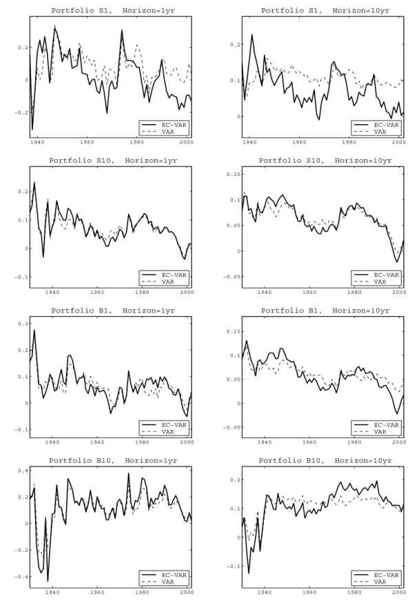
Further, asset return predictability is also altered by the cointegration between dividends and consumption. Return projections’ ¯R2’s for horizons 1, 5 and 10 years implied by the EC-VAR model as well as the alternative, growth-rate specification are reported in Table 4. The EC-VAR specification, on average, is able to explain an average (median) of 11.5% (10.5%) of return variation at one year horizon, and 44.0% (43.5%) of the variation in ten-year returns. Excluding the cointegrating residual significantly lowers the predictability of asset returns and alters the conditional mean of returns. We illustrate this point in Figure 1 by plotting one and ten-year returns predicted by the EC-VAR specification along with the forecasts implied by the alternative VAR model. Predicted conditional means are displayed for the top and bottom market capitalization and book-to-market portfolios. It can be seen that the two specifications produce quite different predictions of future expected returns, especially at longer horizons. That is, the cointegrating residual, included in the error-correction specification, contains distinct information about future returns beyond that in the growth-rate based model. Return innovations, therefore, also differ across the two specifications, and most importantly so will the consumption betas measured from the two alternative models.
As a robustness check, we have also examined direct projections of multi-period compounded dividend growth rates and returns on the EC-VAR versus growth-rate VAR information sets. We do not entertain this method beyond 5-7 years as the number of independent observations in such direct projections decreases rapidly with the horizon. Predictability evidence from these projections is very similar to that discussed above and, for brevity, is not reported. In sum, we find cointegrating residuals to be a significant predictor of both future growth rates and future
returns at short and intermediate horizons.5
The results of this section underscore the importance of cointegration in the measurement of risk and return. As emphasized in this section, temporary deviations of cash flows from the permanent component in consumption, that is cointegration residuals, contain valuable information for predicting dividend growth rates and returns, and thus represent an important component in the calculation of expected returns and betas by horizon. We turn to this point in the following section, and analyze how the risk-return relation changes with the investment horizon.
3.3
Betas and Expected Returns by Horizon
Mean returns for the portfolios at the one-, five-, and ten-year horizons, implied by the EC-VAR, are presented in Table 5. As shown in the table, the general pattern observed in expected returns is preserved across the various horizons. Small firm portfolios tend to earn higher mean returns than do large firm portfolios, and low book-to-market portfolios earn lower expected returns than high book-to-market portfolios. Further, at all horizons, the mean returns exhibit considerable cross-sectional variation; the dispersion in mean returns at the ten-year horizon is though slightly less than that at the one-year horizon.
We now explore the implications of cointegration for the determination of assets’ consumption risks. Table 6 presents betas at various horizons for each of the portfolios; Newey and West (1987) standard errors are given in parentheses. Similarly to mean returns, risk measures implied by the EC-VAR exhibit substantial cross-sectional variation. At the 1-year horizon, the small-firm portfolio beta (4.12) exceeds the large-firm portfolio beta (1.54), and
5In particular, at the one-year horizon, t-statistics on the cointegrating residual in dividend growth projections are significant for 11 out of 20 portfolios. As the horizon increases, the predictive power of the error-correction variable considerably improves: at the five-year horizon, robust t-statistics in dividend growth and return projections become statistically significant for virtually all the portfolios.
the high book-to-market beta (3.89) exceeds the low book-to-market beta (1.81). Further, there is a generally declining pattern in the size dimension and increasing pattern in the book-to-market dimension that is consistent with the pattern observed in mean returns. As the horizon increases, the cross-sectional pattern in these risk measures generally remains the same, although the precision of the estimates suffers. At the 10-year horizon, the small-firm beta (6.54) continues to exceed the large-firm beta (0.34) and the high book-to-market beta (4.33) exceeds the low book-to-market beta (-0.83).
As argued in Section 1, the cointegration parameter is one of the components of the overall consumption beta at each horizon, along with risks arising from transitory fluctuations in dividends and prices. The relative importance of price risks and short-run dividend risks, however, decreases over time, and in the long run, systematic risks in returns should be dominated by permanent risks in assets’ cash flows. We find that this theoretical proposition is strongly supported in the data. While at the one-year horizon, the correlation between assets’ betas and cointegration parameters is about 0.87, by the five-year horizon it already exceeds 0.90, reaching virtually 1 in the limit. Thus, the contribution of the cash-flow component of risks to the beta dominates in the long run. Moreover, even at short horizons, long-run consumption risks in dividends are an important determinant of assets’ betas.
To illustrate the importance of the cointegrating relation between dividends and consumption for measuring expected returns and conditional consumption betas, we compare the evidence discussed above with that implied by the alternative growth-rate based VAR specification. We find that the magnitude of mean returns for the growth-rate VAR specification, reported in Table 5, is somewhat higher relative to the EC-VAR specification but their cross-sectional pattern by horizon is very comparable to that impled by the EC-VAR. However, the betas in the VAR specification, reported in Table 6, significantly differ from the EC-VAR based betas. For comparison, in Table 6 we also present the unconditional
cross-sectional differences in mean returns on size and book-to-market sorted portfolios. This evidence underscores the importance of conditioning information contained in the cointegrating residual in computing assets’ exposures to consumption risks.
Below, we more formally analyze the relation between mean returns and risk measures in the cross-section across various investment horizons.
3.4
Cross-Sectional Risk and Return
In this section we investigate the cross-sectional risk-return relation and explore the ability of various specifications to account for cross-sectional differences in mean returns across various investment horizons. We report and discuss evidence based on our preferred EC-VAR specification, as well as alternative specifications: the standard growth-rate based VAR and the unconditional C-CAPM. Table 7 presents results of estimating the cross-sectional regression (20) for different investment horizons. The market prices of risk are estimated jointly with the time-series parameters via one-step GMM. The reported standard errors of the cross-sectional parameters, therefore, are robust to the estimation error in betas.6
As shown in the table, at the one-year horizon, betas impled by our EC-VAR specification explain 75% of the cross-sectional variation in mean returns with a positive price of risk of 1.19 (SE=0.41). This explanatory power is maintained at the 5- and 10-year horizons, with adjusted
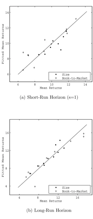
R2 of 0.73 and 0.84 respectively, and prices of risk of 0.73 (SE=0.32) and 0.65 (SE=0.24) respectively. At the very long horizon, i.e., s = ∞, the estimate of the market price of risk remains strongly significant of 0.72 (SE=0.25), and the cross-section of long-run consumption betas accounts for a sizeable portion of the variation in long-run risk premia ( ¯R2=87%). The fit for the one-period and the very long horizon is plotted in Figure 2. Thus, at all horizons,
6In addition, we have constructed bootstrap distributions of time-series and cross-sectional parameters of interest. As bootstrap-based standard errors are very similar to the above-discussed standard errors, for brevity, they are not reported.
the EC-VAR specification explains most of the cross-sectional variation in mean returns across assets. This evidence manifests the empirical importance of the cointegrating relation between dividends and consumption in determining assets’ risk premia not only at long but also at short horizons.
Table 7 also provides the cross-sectional risk-return tradeoff comparison of the EC-VAR relative to the VAR-based specification. As we might expect, given the estimates in the preceding section, the VAR betas have almost no power in explaining the cross-sectional variation in mean returns. In particular, at the one-year horizon, it explains just about 22% of the cross-sectional variation in mean returns and implies although positive, but insignificant, price of risk of 1.278 (SE=1.57). As the horizon extends, however, the ability of the VAR specification deteriorates substantially. At both five and ten-year horizons, it produces negative prices of risks and completely fails to account for the differences in risk premia across assets, as indicated by adjusted R2’s of -0.02 and -0.05 respectively.7
In addition to the conditional beta regressions, Table 7 presents the cross-sectional evidence for the unconditional C-CAPM for the one-year horizon. In contrast to our preferred EC-VAR specification, the unconditional C-CAPM is not able to account for the variation of average returns across the portfolios — the market price of risk is insignificant and the ¯R2 is negative. As the horizon increases, the cross-sectional fit of these unconditional betas remains quite low. For example, at the five-year horizon, the explanatory power of the C-CAPM is only 23%. We do not look beyond the 5-year horizon, as the number of independent observations in such multi-period regressions shrinks rapidly with horizon.
To ensure our results are robust, we consider standard misspecification tests as in
7We find that this evidence is fairly robust if we instead employ a double-sorted set of portfolios. In particular, using 9 portfolio sorted on size and book-to-market characteristics delivers virtually the same magnitudes of market prices of risks as for single-sorted collections of assets, which we discussed in details. The same is true for the cross-sectional ¯R2’s — while the EC-VAR is able to account for more than 50% of the cross-sectional variation in risk premia across various investment horizons, the adjusted-R2’s are virtually zero in the growth-rate VAR setting.
Jagannathan and Wang (1998). Specifically, in addition to our EC-VAR betas, we also include commonly used portfolio attributes: size and book-to-market. We find that the EC-VAR betas remain highly significant, while t-statistics on portfolio-specific characteristics are largely insignificant. In particular, at the first-year horizon, the robust t-statistic on the EC-VAR beta is 2.5; for size and book-to-market characteristics the corresponding statistics are -1.9 and 0.4 respectively. As the horizon increases, the explanatory power of the EC-VAR betas increases, while the significance of both characteristics diminishes. For example, at the ten-year horizon, the t-statistic for our betas is 2.6, and for size and book-to-market attributes are -0.6 and 0.2 respectively. In sum, this finding shows that our EC-VAR based betas are very important for capturing the dispersion in risks across assets.
Our empirical evidence highlights the importance of the cointegration-based specification for understanding the risk-return tradeoff at all investment horizons. The EC-VAR relative to alternative specifications, such as the growth-rate based VAR, incorporates the error-correction term d,tas a predictive variable. This error-correction state variable alters the information set used to predict future returns relative to other specifications of return dynamics, and hence significantly alters the return innovation and conditional betas.
It is worth noting that the implicit assumption (the null hypothesis) behind the EC-VAR specification is that the error-correction term is stationary — all the eigenvalues of theAmatrix are all inside the unit circle. At the point estimates, this critical restriction is satisfied for all 20 portfolios. If this restriction were not satisfied, then our betas could not be constructed for the entire cross-section of assets and the cross-sectional price of risks could not be computed at all horizons. Hence, for evaluating the cross-sectional implications, the null hypothesis that EC-VAR specification leads to stationary dynamics is an important input. In contrast, in the standard VAR, the error-correction mechanism is absent as dividends and consumption are not cointegrated and deviations between them contain a permanent component. This, as discussed earlier, is the key economic difference between these two specifications.
3.5
Long-Run Risks Compensation
Since consumption growth is a covariance-stationary process, its level satisfies a Beveridge and Nelson (1981) decomposition. That is, the consumption process can be presented as a sum of a deterministic trend, a random walk component and a transitory (stationary) component:
ct=µct+Tt+St, (21)
where Tt is the stochastic trend of log consumption, and St is a transitory (or short-run) component. The covariance of the return with consumption (i.e., the beta) can, therefore, be broken into two parts: the covariance with trend shocks (βT,s) and the covariance with transitory shocks in consumption (βS,s),
βT,s= Covt
(rt+1→t+s, Tt+1→t+s)
σT,s2 , and βS,s ≡
Covt(rt+1→t+s, St+1→t+s)
σS,s2 . (22)
The overall beta is just a weighted combination of the two risk measures,
βs ≡βT,s
σT,s2
σ2c,s +βS,s σ2S,s
σ2c,s. (23)
Consequently, at each horizon, the market price of risk reflects the premium for both very long risks and short-run fluctuations in consumption:
1 sEt rt+1→t+s+ 0.5σr,s2 −srt,sf ≡λsβs =λT,sβT,s+λS,sβS,s. (24)
As the horizon increases, transitory consumption shocks die out, and the transitory risk compensation shrinks to zero. Thus, the total risk compensation in the long-run limit (when
s = ∞) provides a measure of the compensation solely for long-run consumption risks, i.e.,
long-run risk-return relation in the cross-section of assets. Subtracting it from the overall risk compensation for a given horizonsallows us to construct the time-horizon profile of risk premia for transitory consumption risks.
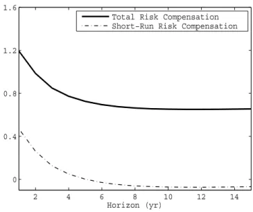
We find that the compensation for long-run risks in consumption is about 60% of the overall compensation at the one-year horizon. Specifically, the estimate of the long-run risk compensation is 0.72 per annum compared to 1.19 at the one-period horizon. Figure 3 plots the compensation for short-run consumption risks along with the total market price of risks for investment horizons up to 15 years. The compensation for transitory fluctuations is small relative to the premium for long-run risks and exhibits a rapid decline as the time horizon grows, starting at about 50 basis points at the first horizon and falling to zero by the 5th year. That is, long-run fluctuations in consumption are the dominant source of the premium for consumption risks in asset markets.
4
Robustness of Evidence
4.1
Alternative Cointegration Specifications
In this section, we discuss the implications of various restrictions on the cointegration specification presented above. In particular, we focus on three alternative specifications relative to our preferred cointegration specification where both δ and τ are unrestricted. In the first, we estimate (12) and (14) under the restrictionδ = 1 for all assets andτ is unrestricted. In the second specification, we impose the restriction that τ = 0 (no time trend) butδ is unrestricted. In the third case, we impose a joint restriction of τ = 0 and δ= 1 across all assets.8
8It the time-series dimension, these restrictions are sharply rejected for the majority of assets. In particular, according to Park (1992) test statistics, single hypotheses ofτ = 0 andδ= 1 are rejected for 13 and 14 portfolios, respectively. The joint null of no time trend and a unit cointegration parameter is rejected for all 20 assets (for all but one portfolio, at the 1% level). Empirical evidence provided in this section reinforces this analysis. We show that imposing restrictions on the long-run dynamics of assets’ dividends and consumption significantly
Results for cross-sectional regressions incorporating these restrictions are presented in Table 8. The first set of columns present results for the first specification, where δ = 1 for all assets (while still allowing for differences in time trends). The results at the one-period horizon are somewhat weaker relative to our preferred case; the price of risk is 1.58 (S.E. = 0.39) and the betas explain 45% of the cross-sectional variation in average returns, as indicated by the
¯
R2. However, as the horizon increases, the explanatory power of the specification deteriorates rapidly. At the two- and five-year horizons, the prices of risk are no longer statistically significant and the explanatory power of the regression is near zero. These results indicate that allowing for heterogeneity in the long-run risk in dividends is important for capturing variation in risk premia not only in the long run, but also the short term.
In the second set of columns, we report results for the second specification, where δ is unrestricted and τ = 0 (no time trend) for all assets. These results represent an improvement over the case in which the cointegration parameter is restricted to be one, and are mostly comparable to our preferred specification. At the first horizon, the estimated price of risk is positive and statistically significant and ¯R2 is of 62%. The price of risk and the explanatory power of the regression remain high as the horizon lengthens. Finally, we have also considered a specification with τ = 0 and δ = 1 for all assets as in Menzly, Santos, and Veronesi (2004). This specification, however, is sharply rejected in the data and, for brevity, we do not report the detailed evidence.
A comparison of our preferred case (unrestricted time trend and cointegration parameter), to the second case where the time trend is eliminated highlights that it is not the time trend per-se but cross-per-sectional heterogeneity that is important for capturing differences in risks across assets at long and short horizons. This is further reinforced by the evidence that when δ = 1, the specification cannot account for the differences in risks at various horizons. As mentioned
limits the ability of the cointegration-based betas to account for the cross-sectional variation in risk premia at all investment horizons.
previously, in the second case (τ = 0 and δ unrestricted) the cointegration parameter equals the ratio of the mean growth rate in the portfolio dividends to the mean growth of aggregate consumption, and hence may tautologically reflect average ex-post returns. Including the time trend purges the effect of mean growth rates in dividends on the cointegration parameter, and ensures that long-run risk measures (that is, δ’s) do not mechanically replicate cross-sectional differences in ex-post average returns. Despite this, if one chooses to restrict τ = 0 for all assets and estimate δ’s under this restriction, this specification produces cross-sectional results that are comparable to our preferred case. This, once again, underscores that it is appropriate heterogeneity inδthat is critical and not merely the inclusion or exclusion of time trends in the cointegration specification. Below, we further highlight the importance of the cross-sectional dispersion in long-run dividend risks, δ’s, using Monte Carlo simulations.
4.2
Monte Carlo Analysis
The results presented above show that the price of risk and ¯R2 are highly significant for our preferred EC-VAR specification. In this section, by means of Monte Carlo simulations, we show that our empirical evidence is robust to alternative specifications and is not likely to be an outcome of a lucky draw. We consider four different Monte Carlos which highlight different aspects of our empirical evidence.
As noted earlier, the cross-sectional heterogeneity in the cointegration parameter is important. Our first Monte Carlo experiment (MC-1) is designed to evaluate if this heterogeneity could arise in a set-up where, in fact, there is none due to either small sample errors or overfitting in small samples. In this experiment, the population value of the cointegration parameter is set at 1 for all assets. We ask the question if such an economy is capable of replicating the cross-sectional evidence that we find across various investment horizons. We simulate all the data, of the sample length, from the EC-VAR specification
that imposes the restriction δ = 1. Using the simulated data we estimate the cointegration parameter and the unrestricted EC-VAR, as we have done in the data. We then use the constructed betas to run cross-sectional regressions and to compute the prices of consumption risk and the ¯R2’s by horizon. Table 9 reports the cross-sectional evidence from this simulation exercise. The table shows that the conditional consumption betas in this case fail to explain the sectional differences in mean returns across almost all investment horizons — the cross-sectional ¯R2’s are very small and the cross-sectional slope coefficients are mostly insignificant. This Monte Carlo experiment, therefore, suggests that our empirical evidence is unlikely to come from a world where long-run cross-sectional dividend heterogeneity is absent. In addition, it underscores the importance of cross-sectional differences in the cointegration parameter for explaining differences in mean returns across all horizons.
In the second Monte Carlo (MC-2), we highlight the importance of the EC-VAR specification relative to the standard VAR specification. As is well known (see Granger and Engle (1987)), imposing a growth-rate based VAR structure when dividends and consumption are cointegrated entails loss of information that emanates from the error-correction mechanism. This can substantially affect the transition dynamics of dividend growth rates and returns and, consequently, the asset’s consumption betas that interest us. The null model that we simulate from is the EC-VAR; we then estimate the standard growth-rate based VAR (using the same specification as discussed earlier) to measure asset betas, price of risk, and the cross-sectional
¯
R2’s. The evidence reported in Table 10 shows that the VAR loses considerable information and, on average, cannot account for the cross-sectional differences in mean returns. In all, this suggests that if the data indeed have an EC-VAR structure then, as documented in our empirical section, the standard-VAR specification (commonly used in empirical work) will fail to measure asset risks.
asks what would one find if one estimates our preferred EC-VAR model.9 It is important to note that under the null of the VAR specification, consumption and dividend growth rates are stationary. However the level of dividend is not cointegrated with the consumption level as they do not share a common stochastic trend. A stationary error-correction variable does not exist as the deviation between dividends and consumption contains a unit root (see Granger and Newbold (1974), and Phillips (1986) and Hamilton (1994)). As the number of time-series observations increases, this unit root will become easier to detect (technically, one of the roots of A matrix will be outside the unit circle for all the assets). This implies that our EC-VAR based consumption betas will not exist in large enough samples. Our focus here, though, is on the modest sample length we observe in the data. We simulate sample lengths of data for 20 portfolios and then attempt to estimate our preferred EC-VAR specification.
We find, that in every each of samples we simulate, the A matrix for at least one of the portfolios implies an explosive path for the estimated error-correction variable. On average, about 3 assets have explosive dynamics and, thus, the EC-VAR conditional betas do not exit for the whole cross-section. Hence, the cross-sectional regression of mean returns on the asset betas cannot be conducted. That is, in this set-up, the distribution of various cross-sectional statistics of interest does not exist even in our modest length samples.10 In addition, we have examined the Monte Carlo distribution of the first-order autocorrelation (ACF(1)) of the estimated cointegration residual from MC-3. We find that the ACF(1) coefficient, even in our modest samples, is very high relative to the data, suggesting as to why some portfolios in a given draw have explosive dynamics. More specifically, for all the portfolios but one, the estimates of the first-order autocorrelation coefficient in the data, reported in Table 2, are well in the left tail (below the 2.5% percentile) of the Monte Carlo distribution. This evidence, and the fact
9Notice that a special case of the null is thei.i.d. growth rates specification. This nested case brings us back to the unconditional C-CAPM specification that, as we have shown, is strongly rejected in the data.
10In particular, the fraction of draws without at least one portfolio having explosive dynamics is zero; the percentage of draws with at least 1 explosive portfolio is 17%, with at least 2 explosive portfolios is 35%, and at least 3 explosive portfolios is 25%. Additionally, probabilities of observing at least 4, 5 and 6 explosive portfolios are 16%, 5%, 2%; for 7 portfolios and above, it is essentially zero.