Florida International University
FIU Digital Commons
FIU Electronic Theses and Dissertations University Graduate School
3-26-2013
Wireless Sensor Network Deployment
Yipeng QuFlorida International University, [email protected]
Follow this and additional works at:http://digitalcommons.fiu.edu/etd
Part of theElectrical and Electronics Commons, and theSystems and Communications Commons
This work is brought to you for free and open access by the University Graduate School at FIU Digital Commons. It has been accepted for inclusion in FIU Electronic Theses and Dissertations by an authorized administrator of FIU Digital Commons. For more information, please [email protected].
Recommended Citation
Qu, Yipeng, "Wireless Sensor Network Deployment" (2013).FIU Electronic Theses and Dissertations.Paper 854. http://digitalcommons.fiu.edu/etd/854
FLORIDA INTERNATIONAL UNIVERSITY Miami, Florida
WIRELESS SENSOR NETWORK DEPLOYMENT
A dissertation submitted in partial fulfillment of the requirements for the degree of
DOCTOR OF PHILOSOPHY in ELECTRICAL ENGINEERING by Yipeng Qu 2013
To: Dean Amir Mirmiran
College of Engineering and Computing
This dissertation, written by Yipeng Qu, and entitled Wireless Sensor Network Deployment, having been approved in respect to style and intellectual content, is referred to you for judgment.
We have read this dissertation and recommend that it be approved.
___________________________________
Jean H. Andrian ___________________________________ Kang K. Yen ___________________________________ Mohammed Hadi ___________________________________ Manos M. Tentzeris ___________________________________
Stavros V. Georgakopoulos, Major Professor Date of Defense: March 26, 2013
The dissertation of Yipeng Qu is approved.
___________________________________ Dean Amir Mirmiran
College of Engineering and Computing
___________________________________
Dean Lakshmi N. Reddi University Graduate School
© Copyright 2013 by Yipeng Qu All rights reserved.
DEDICATION
I dedicate this dissertation to my family and my loving boyfriend. Without their love, patience, understanding and support, the completion of this work would never have been possible.
ACKNOWLEDGMENTS
I would like to express my deepest appreciation to my advising professor, Dr. Stavros V. Georgakopoulos, who has continuously given me guidance and excellent support throughout my entire Graduate and Doctoral studies at FIU.
I would like to thank my committee members, Professor Jean H. Andrian, Professor Kang K. Yen, Professor Manos M. Tentzeris and Professor Mohammed Hadi for serving on my dissertation defense committee and giving enlightening comments.
I am extremely grateful to my loving family in China and my darling boyfriend and proofreader Andrés Miño, who have supported me throughout my research.
Finally, I would like to sincerely thank all of my fellow members of the Electrical and Computing Engineering department and specially all members in our research group: Olutola Jonah, Hao Hu, and Shun Yao for their help and friendship.
ABSTRACT OF THE DISSERTATION WIRELESS SENSOR NETWORK DEPLOYMENT
By Yipeng Qu
Florida International University, 2013 Miami, Florida
Professor Stavros. V. Georgakopoulos, Major Professor
Wireless Sensor Networks (WSNs) are widely used for various civilian and military applications, and thus have attracted significant interest in recent years. This work investigates the important problem of optimal deployment of WSNs in terms of coverage and energy consumption. Five deployment algorithms are developed for maximal sensing range and minimal energy consumption in order to provide optimal sensing coverage and maximum lifetime. Also, all developed algorithms include self-healing capabilities in order to restore the operation of WSNs after a number of nodes have become inoperative.
Two centralized optimization algorithms are developed, one based on Genetic Algorithms (GAs) and one based on Particle Swarm Optimization (PSO). Both optimization algorithms use powerful central nodes to calculate and obtain the global optimum outcomes. The GA is used to determine the optimal tradeoff between network coverage and overall distance travelled by fixed range sensors. The PSO algorithm is used to ensure 100% network coverage and minimize the energy consumed by mobile and range-adjustable sensors. Up to 30% - 90% energy savings can be provided in
different scenarios by using the developed optimization algorithms thereby extending the lifetime of the sensor by 1.4 to 10 times.
Three distributed optimization algorithms are also developed to relocate the sensors and optimize the coverage of networks with more stringent design and cost constraints. Each algorithm is cooperatively executed by all sensors to achieve better coverage. Two of our algorithms use the relative positions between sensors to optimize the coverage and energy savings. They provide 20% to 25% more energy savings than existing solutions. Our third algorithm is developed for networks without self-localization capabilities and supports the optimal deployment of such networks without requiring the use of expensive geolocation hardware or energy consuming localization algorithms. This is important for indoor monitoring applications since current localization algorithms cannot provide good accuracy for sensor relocation algorithms in such indoor environments. Also, no sensor redeployment algorithms, which can operate without self-localization systems, developed before our work.
TABLE OF CONTENTS
CHAPTER PAGE
1 INTRODUCTION ...1
1.1 Problem statement ...1
1.2 Research Objectives and Contributions ...4
1.3 Methodology ...6
1.4 Dissertation Outline ...7
2 RELATED WORK ...10
2.1 Distributed Optimization Algorithms for Sensor Redeployment ...10
2.2 Centralized Optimization Algorithms for Sensor Redeployment ...14
2.2.1 Genetic Algorithm ...14
2.2.2 Particle Swarm Optimization ...17
2.3 Self-localization in Wireless Sensor Networks ...19
2.4 Voronoi Diagram ...23
2.5 Range-Adjustable Sensors ...25
2.6 Energy Consumption ...26
2.7 Summary ...26
3 MODELS AND THEORIES ...27
3.1 Sensing Models ...27
3.1.1 Binary sensing model ...29
3.1.2 Probability sensing model ...30
3.2 Coverage Calculation Model ...32
3.3 Ideal Coverage Model ...35
3.4 Energy Model for Mobile Sensors ...38
3.5 Energy Model for Adjusting Range ...40
3.6 Obstacle Model ...42
3.7 Assumptions ...43
3.8 Summary ...44
4 DISTRIBUTED OPTIMIZATION ALGORITHM DESIGN ...45
4.1 Optimization with Average Relative Position ...45
4.1.1 Assumptions ...45
4.1.2 Optimal coverage distance threshold estimation ...46
4.1.3 Algorithm description ...47
4.1.4 Simulation and results analysis ...54
4.1.5 Conclusions ...63
4.2 Optimization with Weighted Relative Distance ...63
4.2.1 Algorithm description ...64
4.2.2 Simulation and Results ...66
4.3.1 Assumptions ...72
4.3.2 Algorithm Description ...72
4.3.3 Simulation and Results analysis ...79
4.3.4 Conclusions ...88
4.4 Summary ...88
5 CENTRALIZED OPTIMIZATION ALGORITHM DESIGN ...90
5.1 Multi-Objective Genetic Algorithm ...90
5.1.1 Assumptions for MOGA ...90
5.1.2 Algorithm Outline ...91
5.1.3 Algorithm objective and fitness function design ...92
5.1.4 Algorithm description ...94
5.1.5 Simulations and results ...95
5.1.6 Conclusions ...101
5.2 Particle Swarm Optimization ...102
5.2.1 Assumptions for PSO ...102
5.2.2 Optimization goals ...103
5.2.3 Fitness function design ...104
5.2.4 Particle Swarm Optimization ...109
5.2.5 Algorithm Procedure ...110
5.2.6 Simulations and analysis ...111
5.2.7 Conclusions ...116
5.3 Hybrid PSO with distributed algorithm ...116
5.3.1 Algorithm Description ...117
5.3.2 Simulation and Results analysis ...120
5.3.3 Conclusions ...125
5.4 Summary ...126
6 DISTRIBUTED SENSING RANGE ADJUSTMENT ...128
6.1 Assumptions ...128
6.2 Voronoi Diagram ...128
6.3 Algorithm description ...129
6.3.1 Divide and Conquer ...130
6.3.2 Sensing range shortening ...131
6.3.3 Detailed range-adjustment process ...134
6.4 Simulation and Results ...138
6.4.1 Sensing radius adjustment ...138
6.4.2 Communication overhead ...141
6.5 Conclusions ...142
7 CONCLUSIONS AND FUTURE WORK ...143
7.1 Conclusions ...143
7.2 Future Work ...148
LIST OF FIGURES
FIGURE PAGE
Figure 1.1 An example of area coverage by a randomly deployed sensor network. ... 2
Figure 3.1 Difference between binary sensing model and probability sensing model. .... 28
Figure 3.2 Detection probability in Probability model and Binary model. ... 31
Figure 3.3 Coverage calculation for Binary model and Probability model. ... 35
Figure 3.4 Ideal coverage model. ... 36
Figure 3.5 Moving energy calculation illustration ... 39
Figure 4.1 Distance threshold estimation... 46
Figure 4.2 Flow diagram of algorithm. ... 48
Figure 4.3 Example for moving criteria. ... 49
Figure 4.4 Voronoi diagram. ... 52
Figure 4.5 Sensing range adjustment strategy illustration. ... 53
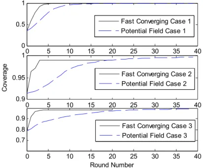
Figure 4.6 Sensing coverage convergence. ... 56
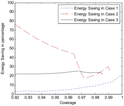
Figure 4.7 Savings in energy consumption. ... 57
Figure 4.8 Initial deployment of sensors in a field with obstacles. ... 58
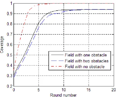
Figure 4.9 Sensing coverage convergence. ... 59
Figure 4.10 Simulation for a sensing field with two obstacles. ... 60
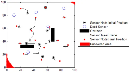
Figure 4.11 Movement traces and final coverage of sensors after self-healing process. .. 62
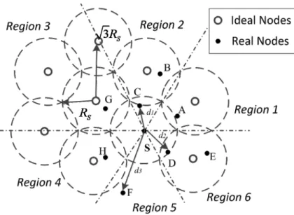
Figure 4.12 Ideal coverage model and region divisions. ... 65
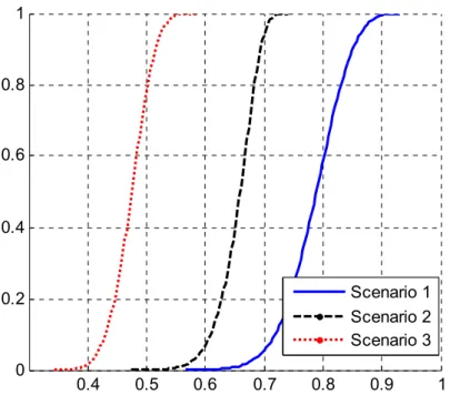
Figure 4.13 Probability of inital coverage ratio in three scenarios. ... 68
Figure 4.16 Probability of final coverage ratio with different noise in sensor locations. . 71
Figure 4.17 Virtual nodes in ideal optimized deployment. ... 75
Figure 4.18 Simulation results for self-relocation algorithm. ... 82
Figure 4.19 Simulation results for average coverage and energy consumption. ... 84
Figure 4.20 Five sensors die out of 20 originally deployed sensors. ... 84
Figure 4.21 Coverage using the for self-healing algorithm. ... 85
Figure 4.22 A sample simulation of self-healing process. ... 86
Figure 4.23 Initial deployment in field with two obstacles. ... 87
Figure 4.24 Statistical coverage result in self-relocation algorithm with obstacles. ... 87
Figure 5.1 Distance calculation when an obstacle appears. ... 93
Figure 5.2 Initial position of 10 randomly deployed sensors... 96
Figure 5.3 Relation between uncovered area and the average travelled distance. ... 97
Figure 5.4 Different Pareto optimal layouts. ... 98
Figure 5.5 Average travelled distance versus the weight coefficient w. ... 99
Figure 5.6 Random deployment of 8 sensors along with the coverage. ... 100
Figure 5.7 Simulation results for 8 sensors with obstacle. ... 100
Figure 5.8 Different Pareto optimal layouts. ... 101
Figure 5.9 Voronoi diagram and sensing radius calculation... 107
Figure 5.10 Sensor random initial deployments. ... 112
Figure 5.11 Best fitness value outcome of PSO algorithm. ... 113
Figure 5.12 Optimal relocation simulation outcome example. ... 114
Figure 5.13 Energy savings of optimization algorithm. ... 115
Figure 5.15 Lifetime optimization when the linear energy model is applied. ... 123
Figure 5.16 Lifetime optimization when the quadratic energy model is applied. ... 123
Figure 6.1 Redundancy and Coverage holes. ... 130
Figure 6.2 Voronoi diagram based sensing radius choosing. ... 132
Figure 6.3 Sensor important definition. ... 133
Figure 6.4 Simulation outcomes with different number of sensors ... 139
Figure 6.5 Example outcome for scenario 2. ... 140
CHAPTER 1
1 INTRODUCTION
1.1 Problem statement
Wireless sensor networks have recently attracted significant interest in the engineering community and among academic researchers. Different sensor network application testbeds have been built by various universities, such as the habitat monitoring sensor networks by the University of California at Berkeley and the College of Atlantic [1], the Zebranet Project for monitoring animal habits by Princeton University [2], and the wireless sensor network monitoring volcano activities in Ecuador by Harvard University, the University of New Hampshire, and the University of North Carolina together [3]. Also, DARPA has built a self-healing, smart minefield based on wireless sensor networks [4].
Different research areas are related to wireless sensor networks, such as sensor network security, coverage, communication, etc. Specifically, this dissertation focuses on the area coverage problem of mobile and wireless sensors. In the area coverage problem, each sensor covers a particular sub-area, and the total covered area of the sensor network is made up of the individual covered areas of each sensor node. Maximizing the total coverage area of the entire sensor network is the major objective of the area coverage problem. The area coverage problem is closely related to the performance of systems in applications, such as, target detection and tracking, monitoring the battlefield, homeland security, personal protection, and animal habit monitoring.
However, there are certain conditions when sensors cannot be deployed deterministically, for example in applications involving areas of natural disasters or harsh environments. Additionally, if the sensing field is very large or has only limited entrance, sensors may not be able to be deployed one by one in precise locations. They may instead be deployed all at once from an aircraft or similar vehicles.
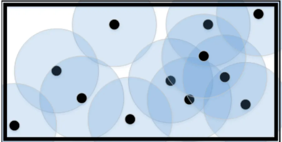
When sensors are randomly deployed, the area-coverage initially provided by the sensor network cannot be guaranteed to be optimal, as in the deterministic deployment. An example of a randomly deployed sensor networks is shown in Figure 1.1. There are twelve sensors deployed in a rectangular sensing field. In the left part of the sensing field, the density of sensors on the left side of the field is less than on the right side. Therefore, the sensing field is not fully covered by the sensors.
Figure 1.1 An example of area coverage by a randomly deployed sensor network. In order to increase the coverage area, redundant sensors are deployed. The redundancy makes the sensor networks have higher density than normal ad-hoc networks. However, it is proved by [5] and [6], that just increasing the sensor density cannot provide coverage with 100% probability. Also, it is costly to maintain the large-scale,
to avoid these problems and still improve coverage after the sensors are randomly deployed.
Nowadays, with the development of Micro-Electro-Mechanical systems (MEMS), sensors have become so small that they have shrunk to the point where they can be carried by pet-sized, mobile robots. Also, certain wireless sensor networks utilize mobile robotic platforms for moving the sensors in a controlled manner. Therefore, instead of increasing the sensing density in a sensor network, the mobile sensors can be used for increasing the coverage.
In addition to the coverage problem of the randomly deployed sensor networks, energy consumption is also a major concern for mobile wireless sensor networks. In most applications, the lifetime of a system is critical to its effectiveness, especially for mobile sensor networks whose mobility systems consume more energy than the other components and processing devices. Energy consumption is a primary constraint for wireless sensor network nodes because most are self-powered by definition. Among the different parts of an individual network node, batteries are the only source of power for its entire life. Some applications are limited to the most essential components and do not have the option of recharging batteries. All of the node actions, such as, sensing, communicating, computing, and moving consume energy. Thus, once the battery or a sensor runs out of power, the sensor node is not useable anymore. This can degrade the quality of service for the entire sensor network.
In this dissertation, we will develop algorithms that relocate the sensors to improve the coverage of randomly deployed sensor networks, while also minimizing the sensor energy consumption so as to prolong the lifetime of the sensor networks.
There is also another concern that complicates the redeployment problem: the robustness of sensor networks. Once deployed, it is expensive and impractical, if not impossible, to replace unusable sensors in applications as the ones described above. Therefore, if an individual sensor node dies, it will affect the entire performance of the sensor network. The death of a sensor node can be attributed to various causes, such as a dead battery, physical damage in the field due to environmental forces, or being destroyed by enemy. If a sensor that covers a very sensitive area dies and no other sensor can cover that area, the sensor network fails its mission of distributing the sensors effectively.
1.2 Research Objectives and Contributions
The objective of the dissertation is to develop relocation algorithms for mobile wireless sensor networks that optimize both coverage and energy consumption. The specific tasks of our research are as follows:
1. Develop distributed algorithms that optimize the coverage and energy used for
carrying the sensors. These algorithms can be performed by the sensor network
without the use of a powerful central node. Therefore, the algorithms must not contain heavy calculations and also should not involve much communication overhead. The algorithms should also consider these three situations:
a) All sensors have very accurate localization systems on them. b) None of the sensors have any localization systems on them.
Different technologies and methods have been developed and implemented for self-localization of wireless sensor nodes. However, in some environments such as indoors, there is still no accurate localization algorithm for wireless sensor nodes. All these cases need to be analyzed and a different set of algorithms need to be developed for them.
2. Develop centralized algorithms for optimizing the coverage of sensor network
and energy consumed for the sensors. These algorithms can have higher
computation requirements and be performed by a central node. The algorithms are only applicable when central nodes exist in the wireless sensor networks. Also, the use of a central node with high computational abilities should also provide better performance than the one provided by distributed algorithms.
3. Develop algorithms using range-adjustable sensors to provider better coverage
and also to save energy by shortening some of the sensors’ sensing radius. These
algorithms are distributed algorithms that only deal with the sensors range but do not relocate them. They can be used in conjunction with the proposed and other existing relocation algorithms to provide energy savings.
4. Enhance all the developed algorithms with the property of self-healing. Whether
a sensor network is capable of functioning well throughout its entire lifetime highly depends on its overall robustness. Algorithms with self-healing can increase the robustness of the system. The algorithms are designed such that when a sensor node dies, due to a drained battery or some physical condition change, the other nodes will adjust their status and react properly to minimize the influence of the sensor node’s death on the sensor network’s entire performance.
5. Ensure our algorithms exhibit rapid convergence. In most monitoring applications, reaction time is very important. The algorithms are designed to have a fast convergence rate when the sensors are first deployed and also when self-healing processes must take place.
6. Evaluate our proposed algorithm. The performance of our algorithms depends on
area coverage, energy consumption, and the convergence speed. Different initial deployments are tested to ensure the convergence of algorithms. Also, we compare and evaluate the performance of our developed algorithm with the existing solutions.
In our work, seven different optimization algorithms are developed, including three distributed algorithms and three centralized algorithms for sensor relocation and one distributed algorithm for sensing range adjustment. All of the algorithms focus on both optimizing coverage with a limited number of sensors and prolonging the lifetime of the entire sensor network. However, this focus is considered differently in various applications and conditions, such as, if a central node exists or whether the sensors can self-locate. These algorithms should be capable of working with both indoor and outdoor monitoring applications, in harsh environments and disaster areas, and in real-time. Simulation results show that in all the different conditions described above, the corresponding algorithms optimize coverage of the sensor network within a reasonable cost of energy.
1.3 Methodology
Firstly, we build the mathematical model for our optimization problem, which involves the maximization of the coverage and the minimization of the energy consumption. Different models related to the problem have been used in our analysis, and we simplify the mathematical model and optimize the solutions. Circle packing and Monte Carlo methods are used to analyze the coverage of the sensor networks.
Secondly, we compare our candidate solutions of the optimization problem with the ideal case of optimal solution and try to generate the solution close to the ideal. Different approaches have been developed in order to achieve the optimum solution.
Thirdly, we develop centralized solutions to the optimization problem. We developed multi-objective Genetic Algorithm and Particle Swarm optimizations algorithms to search for global optimization solutions. Both of these algorithms are heuristic optimization algorithms that will avoid local maxima or minima but provide globally optimal results. The optimum trade-offs are achieved between the conflicting objectives of better coverage and less energy usage.
Fourthly, simulations are done in the Matlab platform. Different random initial deployments are implemented in the simulations and the results are analyzed with probability theory. The simulations are repeated a significant number of times in order to analyze the results by statistical methods.
1.4 Dissertation Outline
The remainder of the dissertation is organized as follows. Chapter 2 discusses the related work. Chapter 3 describes the basic models and theories applied in our work. Two different sensing models are described with respect to coverage calculation. Models and
theories related to energy savings include the energy models of the mobility components and the sensing power model of the sensing components, including range adjustable sensors.
Chapter 4 describes three distributed optimization algorithms: one for sensors with self-location devices, one for sensors without self-location devices, and the other for sensors with inaccurate self-location devices. Simulation results show that in all three cases, the coverage can be optimized. The first algorithm optimizes the average relative distances and provides fast convergence. The second algorithm works without localization system for sensors and provides optimized coverage by a trade-off of energy consumed for moving the sensors. The third algorithm works well when the localization systems of sensors are not accurate.
Chapter 5 discusses our centralized optimization algorithms. Three algorithms are described. The first is based on multi-objective, Genetic Algorithm. The second is based on traditional Particle Swarm Optimization. In the third algorithm, we hybridize the distributed algorithms into a Particle Swarm Optimization and generate a Hybrid PSO, which works uniquely for the sensor relocation problem. The first two centralized algorithms optimize the tradeoffs between coverage and energy consumption of the mobile sensor nodes. The hybrid PSO optimizes the lifetime of sensors and also optimizes the sensing coverage to be very close to 100%.
Chapter 6 discusses a novel sensing range adjustment algorithm that provides near to 100% coverage and also minimizes redundantly covered areas. This algorithm cannot be used for relocating the sensors but can be used cooperatively with our relocation
Chapter 7 summarizes the conclusions and provides recommendations for future research.
CHAPTER 2
2 RELATED WORK
This chapter discusses the related work and the literature view. We separate the related optimization algorithms into two groups with respect to their method of computation: distributed or centralized. After a summary of the existing algorithms, we discuss other related terms such as the self-location techniques in wireless sensor networks, the Voronoi diagram, the range-adjustable sensors, and the obstacle avoidance.
2.1 Distributed Optimization Algorithms for Sensor Redeployment
In the random deployment of sensor networks, distributed algorithms have been used. The most commonly used distributed optimization algorithms for coverage optimization of mobile wireless sensor networks are the virtual force related algorithms [7]-[11].
A potential field method was introduced by Howard, et al., [7], to optimize the coverage of sensor networks. Specifically, in [7], all sensors and obstacles create a virtual potential field. Therefore, every sensor is a point enacted upon by the combined potential field created by all the other sensors and obstacles. Each sensor will be impacted by a composition force from the virtual potential field. The interactive force of a particular potential field of another sensor or obstacle is directly proportional to the square of distance to that sensor or obstacle. The forces can be calculated as:
2 1 i n n i i i r F k r r = −
⋅ (2.1) 2 1 i o o r F k r r = −
⋅ (2.2)where Fn and Fo represents the force due to other nodes and obstacles correspondingly, ri is the directional vector pointing for the center sensor to other sensors or obstacles and ri is its magnitude. It can be seen from the above equation that both forces have a negative sign which means there are only repulsive forces. Sensors will be assigned weights so that they can move according to the virtual forces applied to them as they would in a real physical situation. Virtual frictional effects are also applied so that the algorithm can converge faster. It has been proved that equilibrium state can be achieved in a sensing field with boundaries. As a result, the sensors in the sensing field will rearrange themselves into a more uniform distribution after being randomly deployed, and also, the network’s coverage can be significantly increased.
Sheng, et al., [8] also used the potential field algorithm. In their work, the potential field algorithm was used to relocate the sink nodes, which were carried by mobile robotic devices. After the relocation of the mobile sink nodes, more static sensor nodes could communicate to the sink nodes so that the quality of performance is increased.
Yi Zou, et al., [9], introduced a virtual force algorithm. The major difference between [7] and [9] is that [9] has both repulsive and attractive forces between sensors, whereas [7] only has the repulsive force. The force depends on the distance between sensors and their relative position. The forces can be represented as follow:
( ( ), ) 0 ( / , ) A ij th ij ij th ij ij th R ij ij ij th k d d a if d d F if d d k d a π if d d − > = = + < (2.3)
where dij is the distance between sensors and aij is the direction from the center node to other sensor nodes, and dth is a distance threshold that has a close relation to the sensors’ sensing range. The objective of this algorithm is also to achieve better overall coverage by relocating the mobile sensors.
Different force models have been derived, including the impact of hotspots and obstacles model by Li et al.,[10]. A ranking system has also been applied to the force model, so that the algorithm can be used for varying application requirements.
Wong et al.,[11] improved the virtual force algorithms by applying a back-off delay time in the virtual force algorithm. The back-off delay time is used such that the sensors relocate themselves one-at-a-time in each round of movement. Thus, each sensor will have the most updated position information of the other sensors, including the movement of previous sensors within the current round. In this way, the sensors can move less than if they use the aged location information.
It should be pointed out that the virtual force related algorithms described above require that each sensor knows the exact or relative positions of all other sensors in the network. In other words, location information for sensors is required, and must somehow be communicated throughout the network.
Other deployment algorithms for randomly distributed mobile sensor networks were proposed by Wang et al.,[12], Pac et al.,[13], and Chang, et al.,[14]. These algorithms require that each sensor knows only the relative locations of sensors that are in its communication range, or its neighborhood.
those areas. Three different optimization algorithms have been developed: vector based optimization (VEC), Voronoi diagram based optimization (VOR), and Minimax optimization. The VOR and Minimax have similar performances that are better than the VEC when sensor nodes have low density. These algorithms also used a virtual movement method. With this method, each sensor calculates the future movements of all neighboring sensors and tracks these virtual movements to predict their future locations using the virtual locations. This prediction technique is repeated several times, and then the sensor moves only once. By using the virtual movement method, the total distance of sensor relocation is greatly decreased, along with the energy consumed.
Furthermore, Pac, et al., [13], used a fluid model for sensor relocation. In this algorithm, the author compared the mobile sensor network to a fluid model. The sensors are treated as fluid elements in a continuous medium, which represents the unknown sensing field. This algorithm can optimize the sensing coverage.
Chang, et al. [14] developed a density control coverage optimization algorithm. Each sensor divided its surrounding area into eight, hexagonal subareas, according to the relative direction. Then, the sensor density of each subarea was calculated, according to the number of sensors and the area of obstacles in that subarea. Then, the sensors moved toward the subarea that has the least density.
The deployment algorithms above are not designed to converge fast. However, the convergence speed is an important factor in real time applications.
2.2 Centralized Optimization Algorithms for Sensor Redeployment
The effectiveness of the deterministic deployment of a sensor network is a function of how efficiently it uses the sensor nodes to cover the desired area without any uncovered spots. This problem is related to the Art Gallery problem[15]. The Art Gallery problem is that of positioning the cameras of an art gallery so that the least amount of camera sensors can cover the entire art gallery. This problem is an optimization problem that is Non-deterministic, Polynomial-time hard. The video cameras in the Art Gallery problem are very similar to the sensors in wireless sensor networks. The main difference is that the video cameras have no limit of visual range, as they can see as long as no wall or obstacle blocks their line of sight. However, the sensor nodes always have a limited sensing range.
2.2.1 Genetic Algorithm
Genetic algorithms (GAs) are a type of evolutionary, optimization algorithm. Evolutionary optimization algorithms were first introduced by Barricelli in 1957[16]. GAs are heuristic search algorithms that come from the idea of natural evolution[17][18]. They take the concept of chromosomes, inheritance, mutation, and crossover in natural evolution. In a genetic algorithm, the input variables are treated as chromosome vectors. Different groups of initial variables will be generated. The genetic algorithm evaluates the values of the fitness function related to the input variables and keeps the chromosomes of the best fitness values. The GA simulates mutation and crossover of the chromosomes and always keeps the best values. So the best chromosomes are always inherited. GAs are very useful in obtaining the global maximum without being trapped in
a local optimum. This is because the initial population covers the entire solution space, so that local optimized values will be avoided. They are suitable for solving nonlinear optimization problems and for finding the global optimization value of a fitness function.
Genetic algorithms can be used to solve optimization problems with NP-hard complexity. Also, deterministic deployment algorithms seek to prolong the lifetime of sensor networks by minimizing energy consumption. Some previously developed algorithms have used GAs to obtain optimum deployment of sensor networks.
Jourdan, et al., [19] used a Multi-Objective Genetic Algorithm to optimize the coverage and lifetime of an entire wireless sensor network. In the sensor network in [19], there is only one sink node. All sensors need to transmit data to the sink node directly or through multi-hop communication. Data transmission is the main concern of energy consumption in [19]. So with different communication ranges, the data transmission will have different number of hops, changing the energy consumed. The work presented in [19] deals with the conflict of the goals of minimizing energy consumption and maximizing coverage and uses a Multi-Objective Genetic Algorithm to find the optimal tradeoff between coverage and lifetime. Different optimum layouts are obtained with respect to different sensing-to-communication range ratios.
Jia, et al.,[20] deals with the scheduling problem for redundant sensors to prolong the lifetime of wireless sensor networks. The two objectives of their fitness function are to maximize the coverage and minimize the area covered by more than one sensor. They introduced a non-dominated sorting genetic algorithm (NSGA-II) to solve the optimization problem and minimize the number of sensors that need to be “on” to cover
the maximum area. The other sensors are turned off so that they can save their energy and can be used when other sensors die.
Wang, et al.,[21] focused on improving the problem of selecting dynamic sensor nodes, which was first introduced by Burne, et al.,[22]. The problem is similar to the problem described in [20] but it involves the energy of each sensor in real time, dynamically. The objectives are to optimize the coverage ratio and prolong the lifetime of the entire sensor network. A Hopfield network (NH) is used to reduce the search space of the GA. Compared to the GA, this NH-GA converges faster.
Also, sensing range adjustment and coverage optimization were performed in[23]. The work presented in[23] used the Voronoi Diagram to determine the approximate sensing range of each sensor and then used the GA to optimize the utilization of power.
Liang, et al.,[24] performed the optimization work for wireless sensor networks in 3D environments. In this work, a force driven genetic algorithm was introduced to decide the location of the sensors in order to obtain an optimized coverage and also consider energy savings.
GAs are suitable for optimizing the deployment positions of sensor nodes, scheduling of groups of sensor nodes, and optimizing energy usage such as optimizing the sensing range and communication. GAs are very powerful optimization tools for the wireless sensor networks. However, the main restriction of GAs is they have very high computation complexity; thus, they require powerful CPUs. A normal sensor node usually does not have the ability to do so, and a central node with powerful computational capabilities is always required for GAs.
2.2.2 Particle Swarm Optimization
Particle Swarm Optimizations (PSOs) was first introduced by Kennedy, et al.,[25] in 1995. The idea of a PSO comes from the natural behavior of birds seeking food. When a group of birds are looking for food together, each bird will first look around in the area near itself. Each bird will communicate to the other birds where it finds the most amount of food near its area. Thus, all the birds can know which areas have the most amount of food in their entire, collective feeding area. Birds will continue looking for food in nearby places, especially where the most amount of food had been found in the entire area. PSO algorithms simplify this concept of organized labor. Similar to GAs, a group of candidates will be generated in PSOs from the entire space. Each candidate is a set of vectors that contain the variables related to the problem. The group of candidates will evolve to the combination of personal best fitness and the group global best fitness. This is like the process of the birds seeking food.
Compared to GAs, the PSO has the advantage that it is easier to program and implement, and it has less parameters to control. The PSO has been widely used in wireless sensor networks[26], such as node and base station positioning[27], node localization[28][29][30], data aggregation[31][32], and energy aware clustering[33][34].
PSO has been used in coverage and energy optimizations for non-mobile wireless sensor networks. Wang, et al.,[35] used a parallel particle swarm optimization algorithm for optimizing the energy used by sensors to track targets. The parallel PSO is used for maximizing the coverage and minimizing the energy consumption by turning off the sensors that are far away from the targets. The simulation results showed siginificant improvement in energy efficiency.
The PSO has also been used for relocating mobile sensor nodes[36]-[39]. Bai, et al.,[36], used PSO to optimally relocate sensors that are initially randomly deployed. The objective of their PSO is to optimize the coverage of the sensor network with least amount of sensor movements. Specifically, they studied two different cases of sensors mobility. In the first case, the sensors can move unlimited distance. In second case, the sensors modeled with limited mobility, which means they can only move within a certain maximum distance. The PSO algorithm improved the network’s coverage in both cases, especially in the limited mobility model. Also, the energy spent for the sensors’ movement was greatly reduced.
Wang, et al.,[37], developed a new PSO algorithm, called VFCPSO, which combines the virtual force (VF) algorithms and co-evolutionary particle swarm optimizations (CPSO). In this algorithm, virtual forces are used to update the evolving velocity of each candidate solutions and different, cooperating swarms. The algorithm optimizes the coverage of a network that contains both static and mobile sensors. Compared to the traditional PSO, the VFCPSO can perform better with increasing dimensionality of the optimization problem and decreasing the computation time of the VFCPSO. Simulation results showed that VFCPSO provides a 10% coverage increased compared to the traditional PSO. Huang and Lu [38] also applied the PSO to the coverage optimization of hybrid, wireless sensor networks.
Li, et al., [39] imported selection and mutation to the PSO and named their algorithm Particle Swarm Genetic Optimization (PSGO). Their algorithm aims at improving the density of nodes. Mobile nodes move to cover the uncovered areas
algorithm could increase the coverage by 6%. However, these algorithms do not focus on energy savings and prolonging the lifetime of sensor networks with limited energy resources.
2.3 Self-localization in Wireless Sensor Networks
Self-localization is the ability to know one’s location with respect to some agreed upon reference, and it is very important for wireless sensor networks, since most applications require knowledge of where the data is coming from. It is also important to the coverage optimization algorithms, most relocation algorithms discussed above require knowing at least the relative locations of sensors, and they cannot function if the sensors have no self-localization system. Therefore, sensor localization has become an active research topic in recent years.
There are two types of sensor self-localization methods; one is Fine Grained Localization and the other one is Coarse Grained Localization. The first type usually has less error in the localization results than the second, but it usually involves either higher computational complexity or hardware cost.
A typical Coarse Grained Localization algorithm for wireless sensor networks is the Distance Vector hop (DV-Hop) method introduced by Niculescu[40]. In this algorithm, the distances between nodes are estimated by the least number of hops they need to communicate, where a hop is a communication link used between sensors that form part of a larger segmented transmission path. Since neither the hop distance between each sensor pair is constant, nor are their associated directions always the same, this algorithm can only estimate the approximate area that other nodes are in, and not their
exact locations. Different algorithms are developed to optimize the original DV-Hop. Li, et al.,[41] developed a weighted DV-Hop self-localization scheme that can increase the accuracy of the traditional DV-Hop. Other improved algorithms are [47-51]. [42][43][44][45][46].
Bulusu, et al., [47] introduced a reference-point based, low-cost self-localization algorithm for wireless sensor networks. In this algorithm, base stations, or other types of infrastructures, are located at grid points. They send out beacon signals including their location information to nearby sensors. These sensors use this information to estimate their own location by assuming they are at the centroid, or average location, of all the stations from which they receive beacon signals. If a sensor node can hear from reference nodes located in (x1,y1), (x2,y2),… (xn,yn), the sensor node will self-locate itself as:
1 1 1 1 n est i i n est i i x x n y y n = = = =
(2.4)where (xest,yest) is the estimation location decided by the sensor. Thus, this method does not require the sensors to know or use the strength of the beacon signal, as the exact distance is not calculated. The accuracy depends on the density of the reference points and the distances between them. Furthermore, the accuracy of this method increases as the density of the reference points increases
Xu, et al.,[48] introduced a coarse localization algorithm based on received signal strength indicators (RSSI). In this algorithm, three base stations are placed in different corners of a sensing field that, again, send out beacon signals to nearby sensors. A signal strength map is generated and stored by the individual sensor nodes. In the map, there are
known to the sensor nodes. The individual sensors will compare the received signal strengths of the three base stations with that of the reference nodes and assign to themselves the location of the reference points with the most similar values.
In the Coarse Grained Localization schemes described above, there is not much calculation involved. However, the Fine Grained localization is different. Fine-grained localization algorithms can be classified into three types: received signal strength (RSS) based, time of arrival (TOA) based, and direction of arrival (DOA) based.
In RSS based localization algorithms, radio propagation model equations are used, as the received signal strength between sensors or base stations are directly related to the distance between them. The main process of an RSS based localization algorithm is the determination by the sensors of their locations. First, each sensor receives the beacon from the reference nodes (base stations etc). Then, it calculates the distance to each reference node. Finally, it solves the distance equations to get its own location. The main obstacle of this type of algorithm is that the parameters, especially that of the path loss exponent (also called distance-power gradient), in the equations are not easily obtained due to variations in the environment of sensing field and the uncertainty of channel noise in lognormal fading. Thus, different algorithms are developed to optimize the solutions of the equations and minimize the localization error.
Li, [49] developed an RSS based localization algorithm for unknown distance-power gradients. He used the gradient method to minimize the estimation error. Simulation results show a significant advantage of this algorithm over ones with fixed distance-power gradient values when the distance-power gradient is not accurate. Similar works are also done in [50]
MacDonald, et al., [51] analyzed the RSS based localization algorithm with an isotropic transmitter. They also estimated the distance-power gradient to be 2, which is the free space value. They also use the gradient method to optimize their results. They tested their algorithm with localized, cell phone base stations along Lake Shore Drive in Chicago.
Other relevant RSS-based works are included in the following. Shi, et al., [52] use the steepest descent method to refine the node position of RSS and minimize the influence of the noise. Yao, et al., [53] used Particle Swarm Optimization to increase the localization accuracy. Jia, et al., [54] used Genetic Algorithm to perform the optimization. Amutha, et al., [55] developed a hybrid algorithm that first uses the hop count to approximate the positions of the sensor nodes and then uses RSS to refine the result.
TOA is another distance based localization algorithm. In this type of algorithm, the distance is calculated using the time differences between when the beacon signal is transmitted and when it is received. Radio waves are propagate very fast, thereby requiring a very accurate clock to determine the locations precisely. Therefore, the TOA algorithms have a high cost. The global positioning system (GPS) is a typical application of the TOA localization[56]. Mobile devices use the signal received from satellites to calculate the distance between the satellites and themselves. The satellites also send their own location information, so that the mobile devices can calculate and estimate their own locations. A detailed survey about TOA based localization algorithms is presented in [57]. Other TOA algorithms can be found in [58-60].[58][59][60].
beacon signal they received. This usually requires antenna arrays or some other complicated hardware using directional antennas. Sensors use the location information of the reference nodes and the angle, or direction, at which they received the beacon signal to solve triangulation equations and determine their locations [59-62].[61][62][63][64].
When sensor networks are used indoors, accurate self-localization becomes significantly more difficult. This is primarily due to multipath fading, or signal degradation when radiated through dense materials, such as metal and concrete found in buildings. Various improvements have been implemented to reduce the noise in indoor environments. Pu, et al., [65] used time-series filters to eliminate the noise in RSS localization algorithms. Wu, et al., [66] used radio map filters to deal with noise. Chen, et al., [67] analyzed the obstacles’ influence on the localization systems and derived an error-based improved RSS localization algorithm.
The localization error of wireless sensor networks used indoors is at mimimum 2 meters, in existing manufactured products. This is tolerable if there are not any walls or obstacles that must be taken into account. However, if a sensor node is near a wall, which is about 20 cm thick on average, the previously discussed localization schemes are not able to determine on which side of the obstacle the sensor is located. With this level of uncertainty, most relocation schemes described before cannot function properly for indoor sensor networks.
2.4 Voronoi Diagram
A Voronoi diagram is a method of decomposing an area. Assume there is a set of
entire area into N subareas, and each subarea has a single node inside it. The characteristic of Voronoi diagram is that each subarea is composed of the area closest to the node inside it, as opposed to the other nodes. The generation of the Voronoi diagram requires the location information of all nodes. Voronoi diagrams are very useful in the coverage problem of wireless sensor networks. If each sensor can cover its own Voronoi subarea, the entire sensing field can be covered.
Voronoi diagrams have been used for detecting uncovered areas. Aziz, et al., [68] used PSO to optimize the coverage of wireless sensor networks. Voronoi diagrams are used for calculating whether there are any uncovered areas, so as to calculate the fitness function. Meguerdichian, et al., [69] examined the best-worst case coverage in target tracking in wireless sensor networks. A Voronoi diagram is used for the worst case coverage analysis. The worst case coverage happened when the target traveled along the edge of Voronoi subarea. Boukerche, et al., [70] optimized the centralized Voronoi diagram approach and reduced the computation for coverage problem in wireless sensor networks.
Wang, et al., [12], also used a Voronoi diagram for uncovered area detection in wireless sensor networks. After detecting the uncovered area, sensors move toward that direction, and thus increasing the coverage. Wang, et al., [12], also developed a scheme in which the sensors are always moving to the center of the Voronoi subarea, so that the sensors will have a larger chance to cover the entire Voronoi subarea.
Voronoi diagrams have also been used to optimize the coverage of wireless sensor networks. Li, et al., [71] used Voronoi diagram to assist in reducing the number of
applied the Voronoi diagram on wireless sensor networks to save the energy when range adjustable sensors are used. The Voronoi diagram can help choose the sensing range that is shortest without decreasing the coverage of the entire sensor network.
2.5 Range-Adjustable Sensors
Range-adjustable sensors can change their sensing range by controlling their power. This type of sensor can be used to save energy by shortening the sensing range. There are now some sensors available with range adjustable capabilities, such as some motion detection sensors and photoelectron sensors. Motion detector sensors are very typical sensors that can be found in safety monitoring or in harsh environments.
Wu, et al., [72] studied a coverage problem with range-adjustable sensors. They attempted to minimize the number of sensors and maintain the coverage, in order to lower the energy consumption. Different energy models have been proposed to describe the relationship between the sensing range and consumed energy. A scheduling model has been proposed to achieve the objectives.
Cardei, et al., [73] introduced an energy saving method using range-adjustable sensors. They grouped the sensors into Adjustable Range Set Covers (AR-SC), such that each set can cover the entire desired area. A scheduling scheme was also proposed, so that the energy can be saved and the lifetime of the entire wireless sensor network can be optimized.
Dhawan, et al., [74] also developed algorithms for a similar problem as the one handled by [73]. A mathematical model was proposed and the approximation algorithm of Garg-Konemann was used to determine the approximate solutions. Simulations
showed that their algorithm can increase the lifetime of sensor network by four times compared to the one of [73].
2.6 Energy Consumption
As we described in the first chapter, a common mobile sensor has several components, such as the CPU, memory, battery, sensing device, and mobile device. These components will need to use energy from a battery. It will be very helpful to know the energy consumed by each of the components.
Pei, et al., [75] did a survey on hardware platforms for wireless sensor networks. They summarized the sensor nodes hardware for different applications. They analyzed the energy consumption for different communication protocols and microprocessor platforms. Stojcev, et al., [76] summarized the energy consumed in different types of sensors such as a GPS, a barometric sensor, and a humidity sensor. They also compared the power of some common radio modules. Mei, et al., [77] presented a mobile device for carrying wireless sensor nodes. They analyzed the energy consumed when a sensor node moves straight or turns.
2.7 Summary
This chapter summarized both distributed and centralized algorithms for coverage optimization of wireless sensor networks. We also described some key terms related to coverage optimization: the localization of sensors is critical for the coverage optimization algorithm; the Voronoi diagram is helpful for coverage calculation and energy savings; range-adjustable sensors can also be used for energy saving. Lastly, we discuss the energy consumption of different sensors’ components.
CHAPTER 3
3 MODELS AND THEORIES
This chapter describes the models and theories that are related to the coverage optimization algorithms. The coverage of wireless sensor networks is related to the sensing model used. Different sensing models are introduced in this chapter, and the corresponding methods for coverage calculation are described in the following. We also explain the ideal model for sensor deployment for optimizing coverage, without any uncovered areas in between the sensors. In order to optimize the energy usage in individual wireless sensor nodes of the network, we also describe the energy models for mobile sensors and range adjustable sensors.
3.1 Sensing Models
There are two types of sensors in the real world. The first type of sensor only is concerned about the data at the point where it is located, such as temperature, humidity, and pressure sensors. The second type of sensor has a certain range in which it can detect, such as motion detectors and video camera sensors. In our discussion, we mainly focus on the second type of sensors, because they are more commonly used for area monitoring and safety surveillance.
In the real world, the sensing range of sensors may be irregular due to the obstacles in the environment, such as rain and snow. Fei, et al., [78] researched the irregular sensing range due to the existence of obstacles in the real world and proposed an α-shape range detection model.
However, in order to simplify the analysis and calculation, the sensing range of each sensor is always assumed to be a circular area. Commonly, there are two different types of sensing models used for simulating the performance of sensors [9]: the binary and probability models.
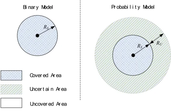
The difference between binary sensing model and probability sensing model is that, in the probability model, if a target is in a certain area, the target may be detected with a certain probability between 0 and 1. However, there is no such area in binary model. In binary model, a target can either be detected or not. This difference between the models is illustrated in Figure 3.1. The notation used is explained below.
Figure 3.1 Difference between binary sensing model and probability sensing model.
RU RS RS Uncover ed Ar ea Cover ed Ar ea Uncer t ai n Ar ea
3.1.1 Binary sensing model
If there is a sensor node S at location (xs, ys), we assume that the sensing range of the sensor S is a circular area with radius RS and centered at (xs, ys). RS is called the sensing radius of node S.
In the binary model, the sensor S is able to detect the target inside its sensing range with a probability 1, and it is not able to detect any target that is outside of its sensing range. Thus, in the binary model, a sensor can detect the target with a probability of 1 if the distance between the target area and the sensor is less than the sensing radius
RS. However, if the distance between the target and sensor is farther than RS, the sensor will have zero probability of detecting it.
Assume a target T is located at coordinate (xt, yt), the probability that the target T will be detected by sensor S in binary model can be expressed in the following equation:
1 0 TS S sb D R p Otherwise ≤ = (3.1)
where psb represents the sensing probability in binary model, DTS is the distance between target T and sensor S which can be calculated as:
2 2
( ) ( )
TS s t s t
D = x x− + y −y (3.2)
There is no transitional period in the binary model. A slight difference in locations may result in a totally different detection output. The binary model is the most simplified model for sensing.
3.1.2 Probability sensing model
In the probability model, unlike the binary model, there is a transitional period between when a sensor absolutely can and cannot detect a target. There will be a certain area for each sensor, in which the sensor cannot tell if a target can be detected. In that area, the target will have a probability to be detected between 0 and 1.
In the probability model, there are two critical distances for a sensor. The first one is RS, which is the same as the one in the binary model. If the distance between the target and the sensor is less than RS, the target can be detected by the sensor with a probability of 1. The second critical distance is RU, which stands for the uncertain range. If the distance between the target and the sensor is in the range between RS and RS+RU, the probability that the target will be detected by the sensor is related to the distance between them. If the distance between the target and sensor is farther than RS+RU, the target will not be detected by the sensor. The mathematical expression of probability model is as followed: 1 0 TS S a sp S TS S U S U TS D R p e R D R R R R D β λ − ≤ = < ≤ + + < (3.3)
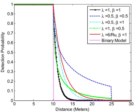
where a =DTS - RS, and λ and β are constants related to the sensors’ hardware properties. The relationship between the probability model, λ, and β is shown in Figure 3.2. In the figure, RS is set to be 10 meters and RU is set to be 25 meters.
Figure 3.2 Detection probability in Probability model and Binary model.
It can be seen in Figure 3.2, that when the distance between the target and the sensor is closer than RS, both binary model and probability model give a detection probability of 1. When the distance is longer than RS and shorter than RS+RU, the binary model gives a 0 probability of being detected, but the probability model will have a gradually decreasing probability. When the distance is longer than RS+RU, both of the sensing models will give a zero detection probability.
Different parameter values result in different transitions regions of the decreasing probability. As it can be seen, when λ and β are both equal to 1, the probability drop from 1 to 0 in about 6 meters, and when λ and β are both equal to 0.5, the probability has not dropped to 0 after 15 meters. In our algorithm, we want to choose the value of λ and β
that can make the probability drop from 1 to 0 gradually in the entire range of RU. Assume β = 1, then λ can be calculated by this equation:
0 5 10 15 20 25 30 0 0.1 0.2 0.3 0.4 0.5 0.6 0.7 0.8 0.9 1 Distance (Meters) D e te ct io n P robabi lit y λ =1, β =1 λ =0.5, β =0.5 λ =0.5, β =1 λ =1, β =0.5 λ =6/Ru, β =1 Binary Model
U
R
e−λ =ε (3.4)
where ε is a small positive value.
We calculate that when λ is equal to 6/RU, εwill be equal to 0.0025. It can be seen in Figure 3.1, when λ = 6/RU and β = 1, the detection probability will drop from 1 to 0 continuously in the entire range of RU. We will use these values in our simulation in the following chapters.
The probability model is more realistic than the binary model and the binary model is the simplified version of probability model when RU is zero. However, the binary model is much easier to analyze.
3.2 Coverage Calculation Model
In Section 3.1, the two sensing models have been described. As the binary model is a special case of the probability model, we can just use one coverage calculation model that fits both of the sensing models.
The definition of coverage ratio (RCoverage) is the ratio of area that can be covered by sensors cooperatively (ACovered) over the entire sensing field (ATotal):
Cov Covera ered t ge To al A A R = (3.5)
The maximum coverage ratio is 1. In the rest of this dissertation, we will use a percentage to describe the coverage ratio.
An area is covered if it can be covered by at least one sensor node or by the joint detection of several sensors. Assume there are N sensor nodes in the entire sensing field, the joint detection probability for a certain area can be calculated as below:
1 1 (1 ) s N Cover s s P = p = = −
∏
− (3.6)where ps can be calculated by equation (3.1) and (3.3) corresponding to the model adopted.
In the binary model, PCover will be either 1 or 0, which means the area will be covered or not. However, in the probability model, PCover will be any value from 0 to 1. A threshold (Pth) is required for judging if an area is covered. If PCover is bigger than Pth, the area is considered to be covered, otherwise, the area is not covered. The value of Pth depends on the application requirement.
Due to the random positions of sensors, the area they cover will be irregular. One method for calculating an irregular area is the Monte Carlo method. The Monte Carlo method is a statistical method for finding numerical results for the problems that are hard to find or do not have analytical results. In the Monte Carlo method, random samples will be evaluated repeatedly. If a sufficient number of samples are evaluated, the results will be very close to the expected value of the outcome [79] [80]..
In the Monte Carlo method, the area of an irregular field can be calculated in the following procedure. First, a regular area that surrounds the target field is chosen. Second, we randomly pick a sufficient number of points in the regular area and judge if each is in the target field. Last, the coverage ratio is calculated with the number of points inside the target field over the number of all sample points. The area will be the coverage ratio multiplied with the area of the regular area.
In our algorithm, we did not sample randomly when calculating the coverage. Instead, we treated the sensing fields as a grid, and used each grid point as a sample point for calculating the coverage. The coverage ratio can be calculated by:
Coverage
n R
N
= (3.7)
where n is the number of grid points that meet the requirement that PCover Pth. It is implied that if Pth is 1, the probability model is equivalent to the binary model.
The accuracy of this method depends on the distance between grids. In our simulations, the sensing field has been divided into 100 by 100 grid points, which means there are 101x101 = 10201 points in total. Therefore, the error in the coverage calculation for our simulations is less than 1%.
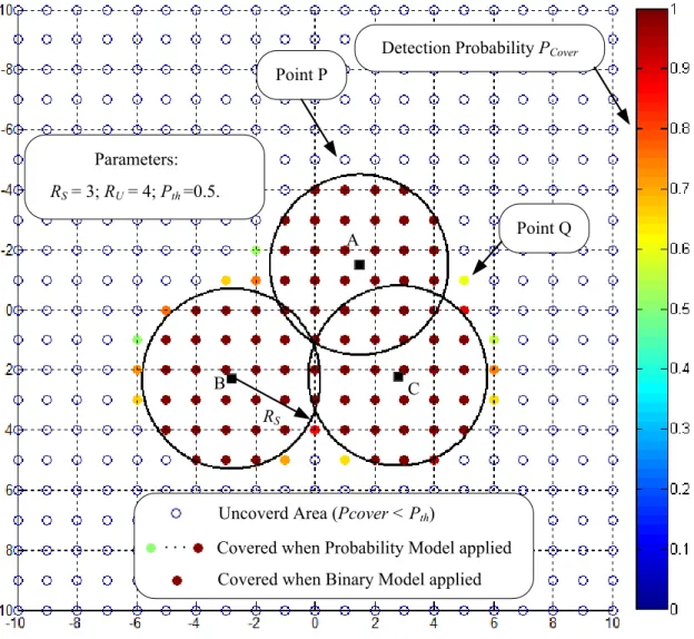
Examples of the coverage calculation in both models are shown in Figure 3.3. In figure 3.3, three sensor nodes A, B and C are deployed in a 20 meter by 20 meter square field. There are 21*21 = 441 grid points in total. The parameters we used here are: the sensing radius is 3 meters, the uncertain radius is 4 meters, and the coverage probability threshold is 0.5. The circles with radius RS represent the real covered areas, with the binary model is applied. It can be seen that all the grid points have probability 1 to be detected. We count the number of nodes that have a detection probability 1, which is 79. So the coverage of binary model is 79/441 = 17.9%. The different color solid points are those that are covered when employing the probability model. The color bar on the right side indicates the probability. All other hollow points are places the probability model cannot cover. The number of grid points covered when applying the probability model is 95, so that the coverage ratio when we use probability model is 21.5%.
Figure 3.3 Coverage calculation for Binary model and Probability model.
Compare point P and Q in Figure 3.3 in probability model. They have similar distances to sensor node A; however, point P is not covered but point Q is covered. This is because Q is in the uncertain range of both sensor A and C. Therefore, the joint detection probability of Q becomes larger than 50%.
3.3 Ideal Coverage Model
Consider a sensing field without any obstacles or attractive areas inside. The deployment of sensors with maximum coverage can be achieved as in [81] and [82]. Boll,
A
B C
RS
Uncoverd Area (Pcover < Pth)
. . . Covered when Probability Model applied
Covered when Binary Model applied Point P
Point Q Parameters:
RS= 3; RU= 4;Pth=0.5.
et al., [81] works on circular packing problems. However, in this work, they only deal with circle packing of adjacent sensors to each other so that a gap will be between each pair circles. Circles are not allowed to overlap. This is not suitable for analyzing the problem of sensor deployment, because in sensor deployment the sensors’ covered areas can overlap.
Wang, et al., [82] analyzed the problem of seamless coverage in sensor networks. Optimal deployment of sensors is achieved when all sensors have the same equal sensing radius. The optimal layout is shown in Figure 3.4. This is an ideal coverage model for the binary sensing model. This can be used for the deterministic deployment of sensors when the boundary of sensing field has a regular shape and there are no obstacles in the sensing field.
Figure 3.4 shows that in the ideal coverage model sensors are deployed regularly with same distance between sensors. The distance between sensors (dth) can be calculated by the sensing radius:
3
th
d = ⋅R (3.8)
a) Binary model
When the binary model is used, R will be equal to the sensing radius RS, therefore, dth can be calculated using RS as below:
3
th S
d = ⋅R (3.9)
b) Probability model
When the Probability model is used, the joint point J will have a detection probability of Pth by the sensor nodes A, B and C. Using the same notations as previous, the radius R can be calculated by solving equation (3.3) and (3.6):
3 1 1 (1 ) s Cover s th s P = p P = = −
∏
− = (3.10) (R Rs) s p =e−λ − β (3.11)Since the distances from sensor node A, B and C to joint point P have same distance, the single detection probability from A, B and C are the same. Equation (3.10) can be simplified to:
(
)
3 1− −1 ps = Pth (3.12) 3 1 1 s th p = − −P (3.13)Also, we are using the parameters in Section 3.2 in which λ = -6/RU and β = 1. R can be solved in the following way:
6 ( ) 3 1 1 s U R R R th e− − = − −P (3.14)
(
3)
ln 1 1 6 U S th R R R= − − −P (3.15)Therefore, dth can be calculated by:
(
3)
3 ln 1 1 6 U th S th R d = R − − −P (3.16)Comparing equation (3.9) and (3.16) for binary model and probability model, when Pth equals to 1 or RU equals to 0, equation (3.16) is equivalent to equation (3.9).
However, this optimal model is ideal because it can only be used for optimizing the deployment without obstacles. If obstacles are present in the sensing field, the problem becomes more complicated. No formulated algorithm is derived when different shapes and numbers of obstacles appear in the sensing field.
3.4 Energy Model for Mobile Sensors
Our algorithms aim at relocating sensor nodes to increase the overall network coverage ratio. In the relocation process, energy will be consumed by each sensor node as they move or turn.
When the weight of sensors and speed are constant, we consider the power consumed in relocating to be constant as well. Therefore, the energy consumed in moving the sensors (Edis) is linear with respect to distance it traveled when acceleration is negligible. Also, every time a sensor node turns, energy will be consumed. The energy consumed for turning (Eturn) is linearly related to the angle sensor node turned. These can be summarized by the following equations:
dis dis total
E
=
k
⋅
D
(3.17)turn