A novel Automatic Optic Disc and Cup Image
Segmentation System for Diagnosing Glaucoma using
RIGA dataset
by
Ahmed Almazroa
A thesis
presented to the University of Waterloo
in fulfillment of the
thesis requirement for the degree of
Doctor of Philosophy
in
Vision Science
Waterloo, Ontario, Canada, 2016
ii
AUTHOR'S DECLARATION
I hereby declare that I am the sole author of this thesis. This is a true copy of the thesis, including any required final revisions, as accepted by my examiners. I understand that my thesis may be made electronically available to the public.
iii
Abstract
The optic nerve head (ONH) of the retina is a very important landmark of the fundus and is altered in optic nerve pathology especially glaucoma. Numerous imaging systems are available to capture the retinal fundus and from which some structural parameters can be inferred the retinal fundus camera is one of the most important tools used for this purpose. Currently, the ONH structure examination of the fundus images is conducted by the professionals only by observation. It should be noted that there is a shortage of highly trained professional worldwide. Therefore a reliable and efficient optic disc and cup localization and segmentation algorithms are important for automatic eye disease screening and also for monitoring the progression/remission of the disease Thus in order to develop a system, a retinal fundus image dataset is necessary to train and test the new software systems.
The methods for diagnosing glaucoma are reviewed in the first chapter. Various datasets of retinal fundus images that are publically available currently are described and discussed. In the second chapter the techniques for the optic disc and cup segmentations available in the literature is reviewed. While in the third chapter a unique retinal fundus image dataset, called RIGA (retinal images for glaucoma analysis) is presented. In the dataset, the optic disc and cup boundaries are annotated manually by 6 ophthalmologists (glaucoma professionals) independently for total of 4500 images in order to obtain a comprehensive view point as well as to see the variation and agreement between these professionals. Based upon these evaluations, some of the images were filtered based on a statistical analysis in order to increase the reliability. The new optic disc and cup segmentation methodologies are discussed in the fourth chapter. The process starts with a preprocessing step based on a reliable and precise algorithm. Here an Interval Type-II fuzzy entropy
iv
based thresholding scheme along with Differential Evolution was applied to determine the location of the
optic disc in order to determine the region of interest instead of dealing with the entire image. Then, the processing step is discussed. Two algorithms were applied: one for optic disc segmentation based on an active contour model implemented by level set approach, and the second for optic cup segmentation. For this thresholding was applied to localize the disc. The disc and cup area and centroid are then calculated in order to evaluate them based on the manual annotations of areas and centroid for the filtered images based on the statistical analysis. In the fifth chapter, after segmenting the disc and cup, the clinical parameters in diagnosis of glaucoma such as horizontal and vertical cup to disc ratio (HCDR) and (VCDR) are computed automatically as a post processing step in order to compare the results with the six ophthalmologist’s manual annotations results. The thesis is concluded in chapter six with discussion of future plans.
v
Acknowledgements
I am grateful to Almighty Allah blessing me to finish this thesis.
I could not find a better word to say thank you, but first of all I would like to
acknowledge my parents for their encouragements and support all the time.
I truly must also acknowledge my supervisor Dr. Vasudevan Lakshminarayanan for
his permanent support, inspiring ideas, encouragements and instructions in my PhD
study. Actually, without his support, this work would never have reached the level
it did.
Moreover, I would like to express my deepest appreciation and gratitude to my co
supervisor Dr. Kaamran Raahemifar for the unlimited guidance and support
throughout my research study.
I also would like to thank the rest of my thesis committee Drs William Bobier and
Simarjeet Saini who has been very helpful and generous.
My gratitude finally goes to my colleagues and friends and other members in school
vi
Table of Contents
AUTHOR'S DECLARATION ... ii Abstract ... iii Acknowledgements ... v Table of Contents ... viList of Figures ... viii
List of Tables ... xv
List of Abbreviations ... xviii
Chapter 1 Introduction ... 1
1.1. Background ... 1
1.1.1. Glaucoma ... 1
1.1.2. Retinal image processing ... 2
1.2. Optic disc and optic cup segmentation... 3
1.3. Publicly available retinal image datasets. ... 4
1.4. Performance Metrics ... 7
Chapter 2 Literature review and thesis objectives ... 10
2.1. Literature review ... 10
2.1.1. Segmentation approaches ... 10
2.2. Objectives of this Thesis ... 51
Chapter 3 RIGA dataset ... 53
3.1. Introduction ... 53
3.2. Images resources ... 54
3.3. Optic disc and optic cup manual annotations ... 54
3.4. Manual annotation segmentation and calculating the geometrical parameters ... 55
3.5. Variation between the 6 Ophthalmologists in the manual annotations ... 59
3.5.1. Optic disc area and centroid ... 59
3.5.2. Optic cup area and centroid ... 63
3.5.3. Horizontal cup to disc ratio (HCDR) ... 68
3.5.4. Vertical cup to disc ratio (VCDR) ... 72
3.5.5. Consolidated results ... 76
3.6. Potential use of RIGA Dataset ... 80
Chapter 4 Optic disc and cup segmentation methodologies ... 81
4.1. Introduction ... 81
vii
4.2.1. Fuzzy set ... 83
4.2.2. An Interval Type-II fuzzy entropy based thresholding ... 83
4.3. Active contours and level set approach ... 86
4.4. Preprocessing ... 89
4.4.1. Localizing the region of interest ... 89
4.5. Processing ... 92
4.5.1. Optic disc boundary segmentation ... 92
4.5.2. Optic cup boundary segmentation ... 110
4.5.3. Comparison between the disc and cup ... 133
Chapter 5 The Cup to Disc Ratios ... 135
5.1. Introduction ... 135
5.2. Horizontal Cup to Disc Ratio (HCDR) ... 136
5.2.1. Results of Bin Rushed dataset ... 140
5.2.2. Results of Magrabi dataset ... 141
5.2.3. Results of MESSIDOR dataset ... 142
5.2.4. Consolidated results for HCDR ... 143
5.2.5. Agreement for HCDR ... 145
5.3. Vertical Cup to Disc Ratio (VCDR) ... 148
5.3.1. Results of Bin Rushed dataset ... 151
5.3.2. Results of Magrabi dataset ... 152
5.3.3. Results of MESSIDOR dataset ... 153
5.3.4. Consolidated results for VCDR ... 154
5.3.5. Agreement for VCDR ... 157
5.4. Final Results (HCDR and VCDR) ... 159
5.4.1. Results of Bin Rushed dataset ... 163
5.4.2. Results of Magrabi dataset ... 164
5.4.3. Results of MESSIDOR dataset ... 165
5.4.4. The final consolidated results ... 166
5.4.5. Agreement for the final ... 169
Chapter 6 Conclusions and future works ... 174
6.1. Conclusions ... 174
6.2. Future work ... 180
Appendix ... 182
viii
List of Figures
Figure 1.1. Optic Disc in fundus image.
Figure 1.2 Retinal images from DRIVE: (a) normal image, (b) pathological image.
Figure 1.3 The relation between the ground truth and automatically annotated area.
Figure 1.4 Measurement of cup-to-disc ratio for a tilted disc.
Figure 1.5 Measurement of the ISNT rule.
Figure 2.1 Flowchart for algorithm proposed in [44].
Figure 2.2 Flowchart for algorithm proposed in [38].
Figure 2.3 Flowchart for algorithm proposed in [34].
Figure 2.4 ODP determination. ((a), (b), and (c)) Original images. ((a1), (b1), and (c1))OD pixels provided by the maximum difference method. ((a2), (b2), and (c2)) OD pixels provided by the maximum variance method. ((a3), (b3), and (c3)) OD pixels provided by the low-pass filter method. ((a4), (b4), and (c4)) Final ODP determination.
Figure 2.5 The calculation process of the circular OD boundary approximation. (R) Red channel; (G) Green channel. R1 and G1: Vessel elimination; R2 and G2: Gradient magnitude image; R3 and G3: Binary image; R4 and G4: Cleaner version of the binary image; R5 and G5: Circular OD boundary approximation.
Figure 2.6 Flowchart for algorithm proposed in [39].
Figure 2.7 Flowchart for algorithm proposed in [36].
Figure 2.8 Flowchart for algorithm proposed in [40].
Figure 2.9 Optic disc segmentation using the proposed method (red), level set method (blue), FCM method (black), CHT method (cyan), and ground truth (green).
Figure 2.10 Flowchart for algorithm proposed in [41].
Figure 2.11 (a) The results (blue: without EF, red: with EF, and green: ground truth). (b)The results (cyan: before 𝛽 -PPA detection, magenta: after 𝛽-PPA detection, red: with ellipse correction, and green: ground truth).
Figure 2.12 Flowchart for algorithm proposed in [37].
Figure 2.13 Flowchart for algorithm proposed in [42].
Figure 2.14 Flowchart for algorithm proposed in [43].
Figure 2.15 Flowchart for algorithm proposed in [35].
ix
Figure 2.17 Flowchart for algorithms proposed in [28, 40].
Figure 2.18 Representative results.
Figure 2.19 Flowchart for algorithm proposed in [66].
Figure 2.20 Flowchart for algorithm proposed in [65].
Figure 2.21 Flowchart for algorithm proposed in [58].
Figure 2.22 Flowchart for algorithm proposed in [62].
Figure 2.23 OD segmentation using proposed method (red), level set method (blue), and FCM method (black) with ground truth (green).
Figure 2.24 Optic cup segmentation using the proposed method (blue), ASM method without vessel removal (red), and level set method (black) with ground truth (green).
Figure 2.25 Flowchart for algorithm proposed in [6].
Figure 2.26 Sample results of the optic disc. From left to right columns: (a) the original images, (b) the manual “ground truth,” and ((c)–(g)) outlines by the MCV, CHT-ASM, EHT, and MDM.
Figure 2.27 Sample results of the optic cup. From left to right columns: (a) the original images, (b) the manual “ground truth,” and ((c)–(e)) outlines by the proposed method before ellipse fitting.
Figure 2.28 Flowchart for algorithm proposed in [61].
Figure 2.29 Flowchart for algorithm proposed in [57].
Figure 2.30 Flowchart for algorithm proposed in [64].
Figure 2.31 Flowchart for algorithm proposed in [60].
Figure 2.32 Flowchart for algorithm proposed in [59].
Figure 2.33 Flowchart for algorithm proposed in [32].
Figure 2.34 Flowchart for algorithm proposed in [63].
Figure 3.1 The manual annotation image segmentation.
Figure 3.2 The geometrical parameters for the optic disc and cup. a) Vertical cup to disc ratio; b) Horizontal cup to disc ratio; c) Disc area and centroid and cup area and centroid.
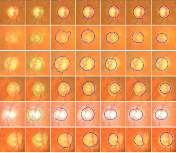
Figure 3.3 Example for a clear cup and disc annotated by 6 ophthalmologists.
Figure 3.4 Results of the geometrical parameters for the 6 ophthalmologists for figure 3.3. X axis represents the number of 6ophthalmologists and Y axis represents the number of pixels for the top graphs and represents ratio for the bottom graphs.
x
Figure 3.5 Example for an unclear cup annotated by 6 ophthalmologists.
Figure 3.6 Results of the geometrical parameters for the 6 ophthalmologists for figure 3.5. X axis represents the number of 6ophthalmologists and Y axis represents the number of pixels for the top graphs and represents ratio for the bottom graphs.
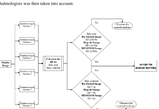
Figure 3.7 Flowchart for the disc annotationsanalysis.
Figure 3.8 Example of the six discannotations.
Figure 3.9 Compering the agreement between the six ophthalmologists in the disc area and centroid annotations in terms of the number of images. X axis represents the number of 6ophthalmologists. Y axis represents the number of agreed images.
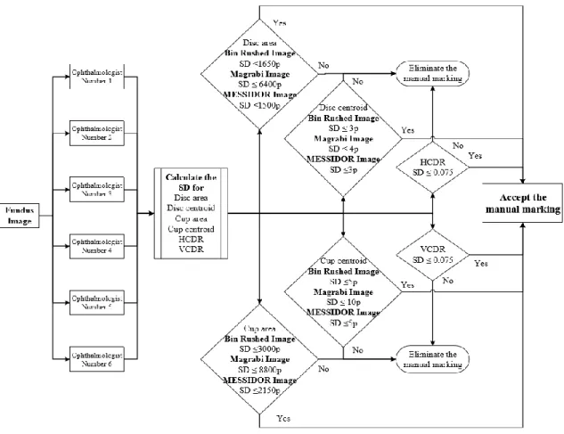
Figure 3.10 Flowchart for the cup annotationsanalysis.
Figure 3.11 Example of the six cup annotations.
Figure 3.12 Compering the agreement in the cup area and centroid among the six ophthalmologists in term of number of images. X axis represents the number of 6Ophthalmologists. Y axis represents the number of agreed images.
Figure 3.13 Comparison between the disc and cup for the agreement in number of the images for every ophthalmologist. X axis represents the number of 6Ophthalmologists. Y axis represents the number of total agreed images.
Figure 3.14 Flowchart for the HCDR annotationsanalysis.
Figure 3.15 Example of the six HCDR annotations.
Figure 3.16 Compering the agreement in the HCDR between the six ophthalmologists in term of number of images. X axis represents the number of 6Ophthalmologists. Y axis represents the number of agreed images.
Figure 3.17 Flowchart for the VCDR annotationsanalysis.
Figure 3.18 Example of the six VCDR annotations.
Figure 3.19 Compering the agreement in the VCDR between the six ophthalmologists in term of number of images. X axis represents the number of 6ophthalmologists. Y axis represents the number of agreed images.
Figure 3.20 Comparison between the HCDR and VCDR for the agreement in number of the images for every ophthalmologist. The X axis represents the number of 6ophthalmologists. The Y axis represents the number of total agreed images.
Figure 3.21 Flowchart for the annotationsanalysis with all the parameters.
Figure 3.22 Example of the six ophthalmologists’ final annotations(Disc, Cup, HCDR and VCDR).
Figure 3.23 Compering the agreement in the total six parameters between the six ophthalmologists. The X axis represents the number of 6ophthalmologists. The Y axis represents the number of agreed images.
Figure 3.24 Comparison between all the parameters as well as the total for the agreement in number of the images for every ophthalmologist. The X axis represents the number of 6ophthalmologists. The Y axis represents the number of total agreed images.
xi
Figure 4.1 General flowchart for the new system.
Figure 4.2 Image histogram.
Figure 4.3 ‘The membership function is shifted over the gray-level range to calculate the amount of fuzziness in each position. The maximum fuzziness indicates the optimal threshold’.
Figure 4.4 ‘A possible way to construct type II fuzzy sets. The interval between lower and upper membership values (shaded area) should capture the footprint of uncertainty (FOU)’ [79].
Figure 4.5 Result for an ultrasound image of carotid artery [85].
Figure 4.6 The results of the localizing algorithm.
Figure 4.7 The flowchart for the disc segmentation algorithm.
Figure 4.8 The disc segmentation procedures for TIFF images.
Figure 4.9 The disc segmentation procedures for JPG images.
Figure 4.10 Flowchart for the analysis of the disc segmentation.
Figure 4.11 Examples for the good disc segmentation results for both TIFF and JPG images.
Figure 4.12 Examples for the bad disc segmentation results for both TIFF and JPG images.
Figure 4.13 The disc accuracy results for all the six ophthalmologists as well as the algorithm for Bin Rushed images set. X axis represents the number of 6 Ophthalmologists and the algorithm. Y axis represents the accuracy (percentage).
Figure 4.14 The disc accuracy results for all the six ophthalmologists as well as the algorithm for Magrabi images set. X axis represents the number of 6Ophthalmologists and the algorithm. Y axis represents the accuracy (percentage).
Figure 4.15 The disc accuracy results for all the six ophthalmologists as well as the algorithm for MESSIDOR images set. X axis represents the number of 6 Ophthalmologists and the algorithm. Y axis represents the accuracy (percentage).
Figure 4.16 The disc accuracy results for all the six ophthalmologists as well as the algorithm for the three images sets. X axis represents the number of 6 Ophthalmologists and the algorithm. Y axis represents the accuracy (percentage).
Figure 4.17 The disc accuracy results for all the six ophthalmologists as well as the algorithm for the three images sets individually. X axis represents the number of 6 Ophthalmologists and the algorithm. Y axis represents the accuracy (percentage).
Figure 4.18 The disc agreement results for all the six ophthalmologists as well as the algorithm for all images sets. X axis represents the number of 6Ophthalmologists and algorithm. Y axis represents the number of agreed images.
Figure 4.19 The disc agreement results for all the six ophthalmologists as well as the algorithm for all images sets. X axis represents the number of 6Ophthalmologists and algorithm. Y axis represents the number of total agreed images.
Figure 4.20 Flowchart for the cup segmentation algorithm. Figure 4.21 The cup segmentation procedures.
xii
Figure 4.22 The function of the cup centroid for X and Y.
Figure 4.23 Flowchart for the analysis of the disc segmentation.
Figure 4.24 Examples for the good cup segmentation results.
Figure 4.25 Examples for the bad cup segmentation results.
Figure 4.26 The cup accuracy results for all the six ophthalmologists as well as the algorithm for Bin Rushed images set. X axis represents the number of 6 Ophthalmologists and the algorithm. Y axis represents the accuracy (percentage).
Figure 4.27 The cup accuracy results for all the six ophthalmologists as well as the algorithm for Magrabi images set. X axis represents the number of 6Ophthalmologists and the algorithm. Y axis represents the accuracy (percentage).
Figure 4.28 The cup accuracy results for all the six ophthalmologists as well as the algorithm for MESSIDO images set. X axis represents the number of 6 Ophthalmologists and the algorithm. Y axis represents the accuracy (percentage).
Figure 4.29 The cup accuracy results for all the six ophthalmologists as well as the algorithm for the three images sets. X axis represents the number of 6 Ophthalmologists and the algorithm. Y axis represents the accuracy (percentage).
Figure 4.30 The cup accuracy results for all the six ophthalmologists as well as the algorithm for the three images sets individually. X axis represents the number of 6 Ophthalmologists and the algorithm. Y axis represents the accuracy (percentage).
Figure 4.31 The cup agreement results for all the six ophthalmologists as well as the algorithm for all images sets. X axis represents the number of 6Ophthalmologists and the algorithm. Y axis represents the number of agreed images.
Figure 4.32 The cup agreement results for all the six ophthalmologists as well as the algorithm for all images sets. X axis represents the number of 6Ophthalmologists and the algorithm. Y axis represents the total agreed images.
Figure 4.33 The total accuracy percentage for the disc and cup versus the total images agreement between the six ophthalmologists as well as the algorithm. X axis represents the number of 6Ophthalmologists and the algorithm. Y axis represents the accuracy (percentage) for (A) and total agreed images for (B).
Figure 5.1 The final algorithm flowchart.
Figure 5.2 Flowchart for the analysis of the HCDR calculation.
Figure 5.3 The algorithm bad HCDR results.
Figure 5.4 The algorithm good HCDR results.
Figure 5.5 The percentage accuracy of the HCDR resultsfor Bin Rushed images set. X axis represents the number of 6Ophthalmologists and the algorithm. Y axis represents the accuracy (percentage).
Figure 5.6 The percentage accuracy of the HCDR results for Magrabi images set. The percentage accuracy of the HCDR resultsfor Bin Rushed images set. X axis represents the number of 6Ophthalmologists and the algorithm. Y axis represents the accuracy (percentage).
Figure 5.7 The percentage accuracy of the HCDR results for MESSIDOR images set. X axis represents the number of 6Ophthalmologists and the algorithm. Y axis represents the accuracy (percentage).
xiii
Figure 5.8 The percentage accuracy of the HCDR results for the total of the three images sets. X axis represents the number of 6Ophthalmologists and the algorithm. Y axis represents the accuracy (percentage).
Figure 5.9 The percentage accuracy of the HCDR for the three images set individually. X axis represents the number of 6Ophthalmologists and the algorithm. Y axis represents the accuracy (percentage).
Figure 5.10 The number of images agreed for the HCDR between the ophthalmologists as well as the algorithm. X axis represents the number of 6Ophthalmologists and the algorithm. Y axis represents the number of agreed images.
Figure 5.11 The total agreed images for the HCDR between the ophthalmologists as well as the algorithm. X axis represents the number of 6Ophthalmologists and the algorithm. Y axis represents the total number of agreed images.
Figure 5.12 Flowchart for the analysis of the VCDR calculation.
Figure 5.13 The algorithm bad VCDR results.
Figure 5.14 The algorithm good VCDR results.
Figure 5.15 The percentage accuracy of the VCDR resultsfor Bin Rushed images set. X axis represents the number of 6Ophthalmologists and the algorithm. Y axis represents the accuracy (percentage).
Figure 5.16 The percentage accuracy of the VCDR resultsfor Magrabi images set. X axis represents the number of 6 Ophthalmologists and the algorithm. Y axis represents the accuracy (percentage).
Figure 5.17 The percentage accuracy of the VCDR resultsfor MESSIDOR images set. X axis represents the number of 6Ophthalmologists and the algorithm. Y axis represents the accuracy (percentage).
Figure 5.18 The percentage accuracy of the VCDR results for all the three images sets. X axis represents the number of 6Ophthalmologists and the algorithm. Y axis represents the accuracy (percentage).
Figure 5.19 The percentage accuracy of the VCDR for the three images set individually. X axis represents the number of 6Ophthalmologists and the algorithm. Y axis represents the accuracy (percentage).
Figure 5.20 The number of images agreed for the HCDR between the ophthalmologists as well as the algorithm. X axis represents the number of 6Ophthalmologists and the algorithm. Y axis represents the number of agreed images.
Figure 5.21 The total agreed images for the VCDR between the ophthalmologists as well as the algorithm. X axis represents the number of 6Ophthalmologists and the algorithm. Y axis represents the number of total agreed images.
Figure 5.22 Flowchart for the algorithm analysis.
Figure 5.23 The algorithm final results for MESSIDOR images set.
Figure 5.24 The algorithm final results for Bin Rushed images set.
Figure 5.25 The algorithm final results for Magrabi images set.
Figure 5.26 The percentage accuracy of the total resultsfor Bin Rushed images set. X axis represents the number of 6Ophthalmologists and the algorithm. Y axis represents the accuracy (percentage).
Figure 5.27 The percentage accuracy of the total resultsfor Magrabi images set. X axis represents the number of 6 Ophthalmologists and the algorithm. Y axis represents the accuracy (percentage).
Figure 5.28 The percentage accuracy of the final resultsfor MESSIDOR images set. X axis represents the number of 6Ophthalmologists and the algorithm. Y axis represents the accuracy (percentage).
xiv
Figure 5.29 The percentage accuracy of the final resultsincluding all the three images sets. X axis represents the number of 6Ophthalmologists and the algorithm. Y axis represents the accuracy (percentage).
Figure 5.30 The percentage accuracy of the VCDR for the three images set individually. X axis represents the number of 6Ophthalmologists and the algorithm. Y axis represents the accuracy (percentage).
Figure 5.31 The number of images agreed for the HCDR between the ophthalmologists as well as the algorithm. X axis represents the number of 6Ophthalmologists and the algorithm. Y axis represents the number of agreed images.
Figure 5.32 The total agreed images for the VCDR between the ophthalmologists as well as the algorithm. X axis represents the number of 6Ophthalmologists and the algorithm. Y axis represents the number of total agreed images.
Figure 5.33 The total number of agreement for HCDR, VCDR and final. X axis represents the number of 6 Ophthalmologists and the algorithm. Y axis represents the number of total agreed images.
Figure 5.34 The percentage accuracy results for all the four parameters. X axis represents the number of 6 Ophthalmologists and the algorithm. Y axis represents the accuracy (percentage).
Figure 6.1 The results of HCDR and VCDR (A) The number of the accepted images (B) the percentage accuracy.X axis represents the number of 6Ophthalmologists and the algorithm. Y axis represents the total agreed images for (B) and the accuracy (percentage) for (B).
Figure 6.2 The final total results (A) The number of accepted images (B) Percentage accuracy. X axis represents the number of 6Ophthalmologists and the algorithm. Y axis represents the total agreed images for (B) and the accuracy (percentage) for (B).
xv
List of Tables
Table 1.1 Performance metrics for optic disc and optic cup segmentation.
Table 2.1 Optic disc segmentation methods.
Table 2.2 Performance results for the optic disc segmentation.
Table 2.3 Categorization optic disc with optic cup segmentation methods.
Table 2.4 Performance results for the optic disc and optic cup segmentation.
Table 3.1 Details of the RIGA dataset. Table 3.2 Notations used for the images.
Table 3.3 The mean SD for the disc area for the three datasets.
Table 3.4The mean SD for the disc centroid for the three datasets.
Table3.5 The number of images agreed between the six ophthalmologists for the disc area and centroid.
Table 3.6The mean SD for the cup area for the three datasets.
Table 3.7 The mean SD for the cup centroid for the three datasets.
Table 3.8The number of images agreed between the six ophthalmologists for the cup area and centroid.
Table3.9The number of images agreed between the six ophthalmologists for the HCDR.
Table 3.10The number of images agreed between the six ophthalmologists for VCDR.
Table 3.11 The number of images agreed among the six ophthalmologists for the consolidated results.
Table 4.1 The localization algorithm results.
Table 4.2 The disc segmentation results for Bin Rushed images set.
Table 4.3 The disc accuracy results for the six ophthalmologists and the segmentation algorithm for Bin Rushed images set.
Table 4.4 The disc segmentation results for Magrabi images set.
Table 4.5 The disc accuracy results for the six ophthalmologists and the segmentation algorithm for Magrabi images set.
Table 4.6The disc segmentation results for MESSIDOR images set.
Table 4.7 The disc accuracy results for the six ophthalmologists and the segmentation algorithm for MESSIDOR images set.
xvi
Table 4.9 The disc accuracy results for the six ophthalmologists and the segmentation algorithm for all the three images sets together.
Table 4.10 The disc number of images agreement between the ophthalmologists as well as the algorithm.
Table 4.11 The cup segmentation results for the 100 images from MESSIDOR images set.
Table 4.12 The cup segmentation results for Bin Rushed images set.
Table 4.13 The cup accuracy results for the six ophthalmologists and the segmentation algorithm for Bin Rushed images set.
Table 4.14 The cup segmentation results for Magrabi images set.
Table 4.15 The cup accuracy results for the six ophthalmologists and the segmentation algorithm for Magrabi images set.
Table 4.16 The cup segmentation results for MESSIDOR images set.
Table 4.17 The cup accuracy results for the six ophthalmologists and the segmentation algorithm for MESSIDOR images set.
Table 4.18 The cup segmentation results for all the three images sets together.
Table 4.19 The cup accuracy results for the six ophthalmologists and the segmentation algorithm for all the three images sets together.
Table 4.20 The cup number of images agreement between the ophthalmologists as well as the algorithm
Table 5.1 The HCDR results for Bin Rushed images set.
Table 5.2 The HCDR results for Magrabi images set.
Table 5.3 The HCDR results for MESSIDOR images set.
Table 5.4 The consolidated results for the HCDR.
Table 5.5 The number of images agreed for the HCDR between the ophthalmologists as well as the algorithm.
Table 5.6 The VCDR results for Bin Rushed images set.
Table 5.7 The VCDR results for Magrabi images set.
Table 5.8 The VCDR results for MESSIDOR images set.
Table 5.9 The consolidated results for the VCDR.
Table 5.10 The number of images agreed for the VCDR between the ophthalmologists as well as the algorithm.
xvii
Table 5.12 The final results for Magrabi images set.
Table 5.13 The final results for MESSIDOR images set.
Table 5.14 The final consolidated results.
Table 5.15 The number of images agreed for the final between the ophthalmologists as well as the algorithm.
Table 6.1 The best accuracy and agreement for all the four parameters and the three images sets. Table 6.2 The worse accuracy and agreement for all the four parameters and the three images sets.
xviii
List of Abbreviations
IOP RNF OCT POAG SD- OCT SAP CDR RNFL ISNT OD OC DRIVE STARE ONH MESSIDOR ORIGA DIARETDB0 DIARETDB1 SP SN ACC PPA DM RAD ROI RMIN SBGFRLS PPA ARIA LoG POI SERI LIBSVM SiMES SCEN MCV CHT-ASM EHT MDM KNN BAYES SVM HCDR VCDR SD FOU PDE GUI Intraocular pressure. Nerve fiber layer.Optical Coherence Tomography. Primary open angle glaucoma.
Spatial domain-optical coherence tomography. Standard automated perimetry
Cup to disc ratio Retinal nerve fiber layer
Inferior (I), superior,(S) nasal (N), and temporal Optic disc
Optic cup
Digital Retinal Images for Vessel Extraction Structured Analysis of Retina
Optic nerve head
Methods to evaluate segmentation and indexing techniques in the field of retinal ophthalmology Online Retinal Fundus Image Dataset for Glaucoma Analysis and Research
The Standard Diabetic Retinopathy Dataset Calibration level Diabetic retinopathy dataset and evaluation protocol
Specificity Sensitivity Accuracy
Positive Predictive Accuracy Dice metric
Relative area difference region of interest
operator which detects the regional minima pixels
Selective Binary and Gaussian Filtering Regularized Level Set Peripapillary atrophy
Automatic retinal image analysis Laplacian of Gaussian
Patches of interest
Singapore eye research institute Library for support vector machine Singapore Malay Eye Study Singapore Chinese Eye Study Chan-Vese model
Circular Hough transform combined with an active shape model Elliptical Hough transform
Modified deformable models K nearest neighbor classifier Bayes classifier
Support vector machines Horizontal cup to disc ratio vertical cup to disc area Standard deviation Footprint of uncertainty partial differential equation
1
Chapter 1
Introduction
1.1.Background 1.1.1. Glaucoma
Glaucoma is a chronic eye disease in which the optic nerve is gradually damaged. Glaucoma is the second leading cause of blindness after cataract, with approximately 60 million cases reported worldwide in 2010 [1]. It is estimated that by 2020 about 80 million people will suffer from glaucoma [1]. If undiagnosed, glaucoma causes irreversible damage to the optic nerve leading to blindness. Therefore, diagnosing glaucoma at an early stage is extremely important for appropriate early management [2-4]. Accurate diagnosis of glaucoma requires three different sets of examinations: (1) evaluation of the intraocular pressure (IOP) using contact (Goldmann tonometry) or noncontact tonometry (“air puff test”), (2) evaluation of the visual field, and (3) evaluation of the optic nerve head [5]. Accurate diagnosis of glaucoma requires additional measurements, that is, gonioscopy and assessment of retinal nerve fiber layer (RNFL) [4]. Since both elevated-tension and normal-tension glaucoma may or may not increase the IOP, the IOP by itself is not a sufficient screening or diagnosis method [6]. On the other hand, visual field examination requires special equipment which is usually available only in tertiary care hospitals that have a fundus camera and possibly an Optical Coherence Tomography (OCT) [6]. In routine practice, patients with primary open angle glaucoma (POAG) can be manifested with inconsistent reports between SD (spatial domain)-OCT and standard automated perimetry (SAP). In the elderly, higher cup to disc (this refers to the optic nerve head) ratio, larger cup volume, and lower rim area on SD-OCT appear to be associated with detectable damage. Moreover, additional worsening in
2
RNFL parameters might reinforce diagnostic consistency between SD-OCT and SAP [7]. Therefore, the optic nerve head examination (cup-to-disc ratio) is a valuable method for diagnosis of glaucoma structurally [8]. The visual field test, on the other hand, diagnoses glaucoma functionally by detecting the damage done to the visual field. Determining the cup-to-disc ratio is a very expensive and time consuming task currently performed only by professionals. Therefore, automated image detection and assessment of glaucoma will be very useful.
There are two different approaches for automatic image detection of optic nerve head [6]. The first approach is based on the very challenging process of image feature extraction for binary classification of normal and abnormal conditions. The second and more common approach however is based on clinical indicators such as cup-to-disc ratio as well as inferior (I), superior(S), nasal (N), and temporal (T) zones rule in the optic disc area [6]. The optic disc is made of 1.2 million ganglion cell axons passing across the retina and exiting the eye through the scleral canal in order to transit visual information to brain [8]. Examining the optic disc helps clarify the relationship between the optic nerve cupping and loss of visual field in glaucoma [8]. The optic disc is divided into three different areas: neuroretinal rim, the cup (central area), and sometimes parapapillary atrophy [9]. The cup-to-disc ratio (CDR) is the ratio of the vertical diameter of the cup to the vertical diameter of the disc [10].
1.1.2. Retinal image processing
1.1.2.1. Fundus photography
Fundus photography is a complicated process. The fundus camera is essentially a low power microscope designed to capture the image of the posterior pole of the eye as well as the whole retina.
3
Fundus photography allows three types of examination: (1) color, in which white light is illuminated on the retina to examine it in full color; (2) red-free, in which the contrast among vessels and other structures is improved by removing the red color through filtering the imaging light; and (3) angiography, in which the contrast of vessels is improved by intravenous injection of a fluorescent dye [11].
1.1.2.2. Optical coherence tomography (OCT)
OCT is an optical signal acquisition method for capturing 3D images with micrometer resolution from within optical scattering media. OCT applies near infrared light and is based on the Michaelson interferometry method.
The long wavelength light has the advantage of penetrating into the scattering medium. OCT is usually used for imaging the retina due to its ability to provide high resolution cross-sectional images [12]. It is also a useful imaging technique in other areas such as dermatology and cardiology [13].
1.2.Optic disc and optic cup segmentation
The Optic Disc (OD) is one of the most important parts of a retinal fundus image [14] (Figure 1). OD detection is considered a preprocessing component in many methods of automatic image segmentation of retinal structures, which is a common step in most retinopathy screening procedures [15]. The OD has a vertical oval (elliptical) shape [16] and is divided into two separate zones: the central zone or the cup, and the peripheral zone or neuroretinal rim [6].
4
Figure 1.1 Optic Disc in fundus image [17]
Changes in the color, shape, or depth of OD are indications of ophthalmic pathologies such as glaucoma [18]; therefore, OD measurements have important diagnostic values [19, 20]. In automated image processing for detection of glaucoma, accurate detection of the central point of OD is important. Furthermore, correct segmentation of OD requires accurate detection of the boundary between the retina and the rim [16]. Pathological cases occurring on the OD boundaries, such as papillary atrophy, influence the segmentation accuracy. Optic Cup (OC) segmentation is further challenged by the density of blood vessels covering parts of the cup and the gradual change in color intensity between the rim and the cup. The kinks in the blood vessels sometimes facilitate detecting the cup boundaries and make it more challenging. Bad image acquisition also affects cup segmentation. Accurate disc and cup segmentation is very important in all pathological cases since errors in disc and cup segmentation may mislead the professionals and hence affect their diagnosis. 1.3.Publicly available retinal image datasets
Most of the retinal optic disc and cup segmentation methodologies presented in the Literature Review chapter were tested on various publicly available datasets, for example, DRIVE, STARE, MESSIDOR, and ORIGA. In this section we provide a brief summary of these datasets.
5 DRIVE Dataset
The Digital Retinal Images for Vessel Extraction (DRIVE) dataset [21] consists of 40 color fundus images. The images were acquired from a diabetic retinopathy research program in the Netherlands. Seven images of the dataset have pathology. Figure 1.2 shows an example of a normal (A) and a pathological (B) image. A Canon CR5 non-mydriatic 3CCD camera with a 45° field of view was used to obtain the images. The images were divided into two groups, a training set and a test set, with 20 images in each group. Three experts manually segmented the images in order to have reference images for evaluating the automatic segmentation techniques by comparing the manually segmented images with those segmented automatically.
(A) (B)
Figure 1.2Retinal images from DRIVE: (a) normal image, (b) pathological image.
STARE Dataset
The Structured Analysis of Retina (STARE) dataset [22] is funded by the US National Institutes of Health. The dataset has 400 fundus images. The blood vessels are annotated in 40 images. The optic nerve head (ONH) is localized in 80 images. A Topcon TRV-50 fundus camera with 35° field of view was used to capture the images.
6 MESSIDOR Dataset
MESSIDOR [23] contains 1200 images in two sets; the images were captured in three ophthalmology departments by a research program sponsored by the French Ministries of Research and Defense. Two diagnoses have been provided by the medical experts for each image, namely, retinopathy grade, and risk of macular edema. A color video 3CCD camera on a Topcon TRC NW6 non-mydriatic retinography with a 45° field of view was used to capture the images. The images are saved in uncompressed TIFF format.
ORIGA Dataset
The Online Retinal Fundus Image Dataset for Glaucoma Analysis and Research (ORIGA) [24] consists of 650 images acquired through Singapore Malay Eye Study (SiMES). Critical signs for glaucoma diagnosis are annotated. SiMES is conducted by the Singapore Eye Research Institute (SERI) [25]. The images were annotated by experts by employing “key nodes” which are imagine landmarks along the disc boundary and cup boundary and were stored in a centralized server. The dataset includes 168 glaucomatous and 482 non-glaucoma images.
DIARETDB0 Dataset
The Standard Diabetic Retinopathy Dataset Calibration level 0 DIARETDB0 [26] consists of 130 color fundus images, 20 normal images, and 110 images with signs of diabetic retinopathy, acquired from the Kuopio University Hospital in Finland. The images were captured by a digital fundus camera with 50° field of view.
DIARETDB1 Dataset
The diabetic retinopathy dataset and evaluation protocol DIARETDB1 [27] consists of 89 color fundus images acquired from the Kuopio University Hospital in Finland. The dataset consists of 84 images with diabetic retinopathy and 4 normal images. The images were captured by a digital
7
fundus camera with 50° field of view. Four experts annotated the microaneurysms, hemorrhages, and hard and soft exudates.
1.4.Performance Metrics
The outcome of optic disc segmentation process is pixel based. Figure 1.3 shows the three distinctive areas: (1) the true positive area representing the overlapping area between the manually annotated (ground truth) and automatically annotated (segmented image) areas, (2) the false negative area where a pixel is classified only in the manually annotated area, and (3) the false positive area where the pixel is classified only in the automatically segmented area. Sensitivity measures the proportion of the actual positives which are correctly identified. A higher sensitivity value implies a higher validity of results [28]. On the other hand, there are different measurements used in image classification of the optic disc and optic cup segmentation to determine whether an image is normal or glaucomatous. Cup-to-disc ratio is defined as the ratio of vertical distances between pixels at the highest and lowest vertical position inside the cup and disc region [29] (Figure 1.4). Table 1.1 summarizes the OD and OC segmentation algorithms performance metrics. Various methods are used for image classification which is a clinical assessment of the ISNT rule for the optic nerve. The ISNT rule is considered to be an observer to the gradual decrease or no change in rim width at the following position order: inferior (I) ≥ superior (S) ≥ nasal (N) ≥ temporal (T) (Figure 1.5).
8
Figure 1.3 The relation between the ground truth and automatically annotated area [9].
Figure 1.4 Measurement of cup-to-disc ratio for a tilted disc [30].
9
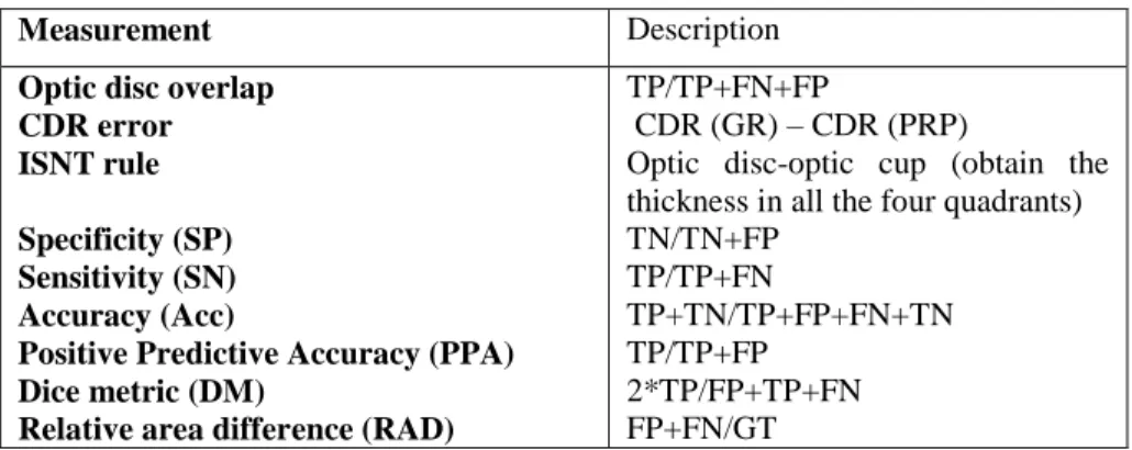
Table 1.1 Performance metrics for optic disc and optic cup segmentation.
Measurement Description
Optic disc overlap CDR error ISNT rule Specificity (SP) Sensitivity (SN) Accuracy (Acc)
Positive Predictive Accuracy (PPA) Dice metric (DM)
Relative area difference (RAD)
TP/TP+FN+FP
CDR (GR) – CDR (PRP)
Optic disc-optic cup (obtain the thickness in all the four quadrants) TN/TN+FP TP/TP+FN TP+TN/TP+FP+FN+TN TP/TP+FP 2*TP/FP+TP+FN FP+FN/GT
As mentioned before, sensitivity is the probability of an abnormal class to be identified as abnormal. Specificity however, is the probability of a normal class to be identified as normal. Accuracy represents the ability or quality of the performance. The positive predictive accuracy represents the precision in detecting normal and abnormal cases. The true negative represents the number of normal images identified as normal, while false negative represents the number of glaucoma images identified as normal. True positive represents the number of glaucoma images identified as glaucoma and false positive represents the number of normal images identified as glaucomatous [32].
In this chapter we have reviewed the methods for diagnosing glaucoma as well as the methods used to take the images of the eye fundus and various datasets of retinal fundus images that are publically available. In addition, the performance matrices used to compute the accuracy of the automatic systems have been introduced.
10
Chapter 2
Literature review and thesis objectives
2.1.Literature review
Different techniques have been used for optic disc (OD), optic cup (OC), or optic disc with optic cup segmentation. In this chapter, the OD and OC segmentation methodologies that automatically detect OD and OC boundaries are critically reviewed. These techniques help professionals with diagnosing and monitoring glaucoma by providing them with clear and accurate information regarding the ONH structure. The uniqueness of this literature review is in demonstrating the segmentation methodology by creating a flowchart for each technique. In this chapter the algorithms applied for OD and OC segmentation are introduced and the pros and cons of each method are discussed. Suggestions for future research are also provided.
2.1.1. Segmentation approaches
Various techniques have been used in image processing methodologies of optic disc and optic cup segmentation in the literate. These techniques for segmentation are, thresholding, edge-based methods, and region-based methods [33]. Here, three segmentation methodologies are considered: (1) optic disc segmentation approaches, (2) optic cup segmentation approaches, and (3) optic disc and optic cup segmentation together. While most algorithms are concerned with just optic disc segmentation, few are concerned with optic cup segmentation and even fewer with optic disc and optic cup segmentation together.
11 2.1.1.1. Optic Disc segmentation approaches
Optic disc extraction or segmentation is performed using segmented reference images called “ground truth” on which the optic disc is accurately annotated by ophthalmologists. The OD processing includes two main steps: localization (detecting the center point of OD) and segmentation (detecting the disc boundary) [34]. Different OD detection and segmentation algorithms have already been introduced; however, many of these algorithms have a number of limitations [35] such as using images with a clear color variation across OD boundary. Preprocessing methods are important steps for analyzing an image by enhancing the image and finding the region of interest (ROI). The OD segmentation approaches are summarized in Table 2.1 and their results are shown in Table 2.2.
Table 2.1 Optic disc segmentation methods.
Authors Year Image processing technique Performance
metrics
Dataset Number of Images
Lupascu et al. [36] 2008 Circles passing through three noncollinear points Success rate DRIVE 40 Youssif et al. [16] 2008 Normalized DFI by means of a vessels’ direction
matched filter
Success rate STARE 81
Zhu and Rangayyan [37]
2008 Edge detection using canny and sobel methods and through transform
Success rate DRIVE STARE
40 82 Welfer et al. [38] 2010 Adaptive morphological approach Overlap (Acc) DRIVE
DIARETDB1
40 89 Aquino et al. [34] 2010 Morphological, edge detecting, and feature extraction
techniques
Overlap (Acc) MESSIDOR 1200 Tjandrasa et al. [39] 2012 Hough transform and active contours Overlap (Acc) DRIVE 30
Yin et al. [40] 2011 Model based segmentation Overlap (Acc) ORIGA 650
Cheng et al. [41] 2011 Peripapillary atrophy elimination Overlapping error
ORIGA 650
Lu [35] 2011 Circular transformation Overlap (Acc) MESSIDOR
ARIA STARE
1200 120
81
Dehghani et al. [42] 2012 Histogram matching Success rate DRIVE
STARE Local
40 81 237 Zhang et al. [43] 2012 Projection with vessel distribution and
appearance characteristics
Success rate DRIVE 40
Fraga et al. [44] 2012 Fuzzy convergence and Hough transform Success rate VARIA 120 Sinha and Babu [45] 2012 Optic disc localization using L1 minimization Overlap (Acc) DIARETDB0
DIARETDB1 DRIVE
130 89 40
Kumar and Sinha [28]
2013 Maximum intensity variation Overlap (Acc) SN
MESSIDOR DIARETDB0
40 130
12
Table 2.2 Performance results for the optic disc segmentation.
Authors Year Dataset Sensitivity Average overlapping
Overlap error
Success rates (Acc) Computation time (s) Lupascu et al. [36] 2008 DRIVE 95% localization 70% identification of OD 60 Youssif et al. [16] 2008 DRIVE STARE 100% localization 98.77% localization 210 Zhu and Rangayyan [37] 2008 DRIVE STARE 92.5% 40.24% N/A Welfer et al. [38] 2010 DRIVE DIARETDB1 100% 97.7% 1083 Aquino et al. [34] 2010 MESSIDOR 99% localization 86% segmentation 1.67 5.69
Yin et al. [40] 2011 ORIGA 11.3% N/A
Cheng et al. [41] 2011 ORIGA 10% N/A Lu [35] 2011 MESSIDOR ARIA STARE 98.77% detection 97.5% detection, 91.7% segmentation 99.75% detection, 93.4% segmentation 5 Tjandrasa et al. [39] 2012 DRIVE 75.56% N/A Fraga et al. [44] 2012 VARIA 100% localization 93.36% segmentation 0.6 Dehghani et al. [42] 2012 DRIVE STARE Local 100% 91% 98.9% 27.6 Zhang et al. [43] 2012 DRIVE Self-selection STARE DIARETDB0 DIARETDB1 100% 97.5% 91.4% 95.5% 92.1% 13.2 Sinha and Babu [45] 2012 DIARETDB0 DIARETDB1 DRIVE 96.9% 100% 95% 3.8 Kumar and Sinha [28] 2013 MESSIDOR DIARETDB0 93% 0.895 90
Fraga et al. [44] presented a methodology for OD segmentation containing different stages (Figure 2.1). In order to reduce contrast variability and increase process reliability, the retinal image was normalized by means of the retinex algorithm [46]. Two different techniques were used to localize the optic disc: (1) analyzing the convergence of the vessels [47] to detect the circular bright shapes, and (2) detecting the brightest circular area based on a fuzzy Hough transform [48]. After detecting the OD, the segmentation techniques were conducted using the region of interest specified by a difference of Gaussian filter. The vessel tree boundaries were segmented by Canny filter to compute the edges. The vessel edges from the Canny output were suppressed using the vessel tree
13
segmentation. Finally, the histogram information was included to measure the accuracy of segmentation. The methodology was evaluated on 120 images and achieved 100% of OD localization for both fuzzy convergence and Hough transform. Using brute force search, the segmentation success rates were 92.23% and 93.36% for the fuzzy convergence and Hough transform, respectively. The aforementioned OD segmentation approach did not involve pathologic retinal images affecting the OD. This is a limitation which should be addressed in the future work in order to develop a robust methodology.
Figure 2.1 Flowchart for algorithm proposed in [44].
Welfer et al. [38] present a new adaptive method based on a model of the vascular structure using mathematical morphology for the OD automatic segmentation (Figure 2.2). This methodology has two main stages: (1) detecting OD location using the information of the main vessels arcade, where the vessels were detected to determine the foreground and background of the green channel image.
14
In this stage, the RMIN operator (which detects the regional minima pixels) was used to identify the background region; (2) detecting the optic disc boundary. In order to detect the OD boundary using the watershed transform, an internal point to the optic disc and other points in vicinity of the internal point were identified based on the previously detected vascular tree and using the following three steps: (1) using a specific algorithm to find the OD position and to determine whether it is on the right or left side of the image (morphological skeleton and pruning cycle are used in this step), (2) locating the optic disc by removing the less important vessels from the pruned image, (3) describing the shape of the optic disc. The methods were tested on 40 images obtained from DRIVE dataset and 89 images from DIARETDB1 dataset. The success rate in optic disc localization was 100% and 97.75% for the DRIVE and DIARETDB1 datasets, respectively. Future work should consider detecting other important retina structures, such as fovea, based on the proposed method.
15
Aquino et al. [34] proposed a new algorithm for OD segmentation (Figure 2.3), where the localization methodology obtains a pixel from the OD called optic disc pixel. The methodology contains three different detection methods (Figure 2.4). Each method has its own OD candidate pixel, and the final pixel was chosen by a voting procedure. The green channel has been selected since it provides the best contrast. Two of the three detection methods are called maximum difference method and maximum variance method. In general the maximum variation occurs between the bright region (OD) and the dark region (blood vessels in the disc). Therefore, the maximum variation was used to select the OD pixel of those two methods. In addition, the statistical variance for every pixel was calculated in the maximum variance method and the bright pixels were obtained by blue channel thresholding via Otsu method [49]. The last method was low pass filter method, where the OD pixel was the maximum gray level pixel in the filtered image.
16
Figure 2.4 ODP determination. (a), (b), and (c): Original images; (a1), (b1), and (c1): OD pixels provided by the maximum difference method; (a2), (b2), and (c2): OD pixels provided by the maximum variance method; (a3), (b3), and (c3): OD pixels provided by the low-pass filter method; (a4), (b4), and (c4): Final ODP determination.
Finally, the maximum variance method has been chosen to have the final OD pixel according to the voting procedure. On the other hand, the OD segmentation methodology was applied on two “red” and “green” components and the better segmentation was selected (Figure 2.5). The procedure was based on removing the blood vessels by employing a special morphological processing and then applying edge detection and morphological techniques to obtain a binary mask of the OD boundary candidates. Finally, the circular approximation of the OD was computed using a circular Hough transform. The methodology was evaluated using the publicly available MESSIDOR dataset. The localization was successful in 99% and the segmentation was successful in 86%. The current research is concentrated on improving the algorithm for executing a controlled elliptical deformation of the obtained circumference.
17
Figure 2.5 The calculation process of the circular OD boundary approximation. (R) Red channel; (G) Green channel. R1 and G1: Vessel elimination; R2 and G2: Gradient magnitude image; R3 and G3: Binary image; R4 and
G4: Cleaner version of the binary image; R5 and G5: Circular OD boundary approximation.
Tjandrasa and colleagues [39] applied the Hough transform as an initial level set for the active contours for optic disc segmentation. The algorithm procedure is shown in Figure 2.6. The OD segmentation steps started by converting the image into a grayscale image and then implementing the image preprocessing (image enhancement). Therefore, homomorphic filtering was applied to reduce the effect of uneven illumination. Homomorphic filtering has two stages: (1) applying a Gaussian low pass filter, and (2) obtaining the filtered edge by performing dilation. The blood vessels are removed in the next step to facilitate the segmentation process. The threshold was applied to detect the low pixel values in the image and followed by applying the median filter to blur the blood vessels. The next step in OD segmentation was detecting a circle which matches the location of OD by performing a Hough transform. Subsequently, an active contour model was used to obtain OD boundaries that are as close to the original OD boundaries as possible. The active contour model was applied with a special processing termed Selective Binary and Gaussian Filtering Regularized Level Set (SBGFRLS) [50]. The algorithm achieved 75.56% accuracy using 30 images from DRIVE dataset. Further work can be done to segment the cup disc in order to classify the images into normal and glaucomatous.
18
Figure 2.6 Flowchart for algorithm proposed in [39].
Lupascu and colleagues [36] presented an alternative technique (Figure 2.7) to detect the best circle that matches the OD boundary. The technique used a regression based method and texture descriptors to identify the circle which fits the OD boundary. The variation in the intensity of pixels described the appearance of the OD, and therefore this fact was utilized in the algorithm. Since the color fundus images have a dark background, the background pixels were not considered. A mask image was computed with zero values for background pixels and one for the foreground pixels. The maximum intensity pixels within the green component provide the highest contrast, and therefore were selected. The initial point was established based on the center of the mass of the region, where eight directions were considered. The directions were obtained by moving counterclockwise in steps of 45°. Each direction was based on the rapid variation of intensity. Three points were considered for each direction; thus in total there were 24 points. The Euclidean distances (the distances between the initial point and each of the 24 points of interest) were computed and their mean value was calculated. The circles were created using three non-collinear points. Hundreds of circles were obtained; however, based on their specific properties, less than twenty circles were selected as the better ones and the rest were removed. Using bilinear filtering, the selected circles were mapped into polar coordinate space. The next step was to find the maximum derivatives in 𝑦 direction by applying the linear least squares fitting technique. The correlation coefficient was computed to measure the quality of the fitting. The circle with the
19
maximum correlation coefficient was chosen as the best circle matching the OD. The algorithm was tested on 40 images. An ophthalmologist manually annotated the ground truth of OD boundary using the standard software to select some pixels on the OD boundary. The success rate was 95% for OD localization and 70% for OD contour (circle) identification. This method caused false detection of OD in low quality images; therefore, further study is needed to improve the algorithm by refining the selection of the initial points.
Figure 2.7 Flowchart for algorithm proposed in [36].
Yin et al. [40] have recently proposed a novel technique that consists of edge detection, circular Hough transform, and a statistical deformable model to determine OD (Figure 2.8). The Point Distribution Model was utilized to model the shape of the disc using a series of landmarks. A preprocessing step was performed to analyze the image and reduce the effect of blood vessels. The optimal channel was also selected by applying a voting scheme based on heuristics.
Subsequently, the OD was approximated by a circle using circular Hough transform to determine the optic disc center and diameter. Ultimately, the statistical deformable model was applied to fine-tune the disc boundary according to the image texture. The direct least squared ellipse fitting method was executed to smooth the OD boundary (Figure 2.9). The ORIGA dataset was used to
20
test the algorithm. The average error in the overlapping area was 11.3% and the average absolute area error was 10.8%.
Figure 2.8 Flowchart for algorithm proposed in [40].
Figure 2.9 Optic disc segmentation using the proposed method (red), level set method (blue), FCM method (black), CHT method (cyan), and ground truth (green).
Cheng et al. [41] proposed an OD segmentation method based on peripapillary atrophy (PPA) elimination. The algorithm included three parts: edge filtering, constraint elliptical Hough transform, and 𝛽-PPA detection (Figure 2.10). Extracting the region of interest and detecting the edges of OD were the initial steps in this algorithm. In the aforementioned steps, a low pass filter was applied to remove the noise, and then the first derivative from each row of the region of interest
21
(ROI) was computed. The first PPA elimination was edge filtering (EF). There are two types of PPA: 𝛼 and 𝛽. 𝛼-PPA is pigmentary and includes a structural irregularity of retinal pigment epithelial cells (darker than OD), while 𝛽-PPA is a complete loss of retinal pigment epithelial cells (similar color to OD). The 𝛼-PPA was detected simply by comparing the ROI with the threshold, i.e., the mean intensity in the ROI, followed by a morphological closing processing. Due to the elliptical shape of PPA together with OD, a second elimination of PPA was conducted by a constrained elliptical Hough transform. Finally, the third PPA elimination was conducted by 𝛽- PPA detection. 𝛽-PPA is much more difficult than 𝛼-PPA due to the similarity of its color with that of OD. To avoid false segmentation between the PPA and OD, a ring area was determined from the detected disc boundary and was divided into quarters. Inspired by the texture within 𝛽 -PPA, the local maximums and minimums were extracted within the ring and were named as feature points. 𝛽-PPA was considered present in a quadrant if the number of feature points in a quadrant exceeded the threshold. The threshold level was obtained by comparing the cases with and without 𝛽-PPA. Then the edge points along the detected disc boundary were removed from the quadrant. Finally, the constrained elliptical Hough transform was reapplied to obtain the new disc boundary (Figure 2.11). The ORIGA dataset with 200 images with PPA was used to evaluate the algorithm. Results showed an average overlapping error of 10%, an average absolute area error of 7.4%, and an average vertical disc diameter error of 4.9%. In the future studies, the method should be reapplied to segment OC for diagnosis of glaucoma.
22 (A)
(B)
Figure 2.11 (a) The results (blue: without EF, red: with EF, and green: ground truth). (b)The results (cyan: before 𝛽 -PPA detection, magenta: after 𝛽-PPA detection, red: with ellipse correction, and green: ground truth).
Zhu and Rangayyan [37] proposed an automated segmentation method based on Hough transform to detect the center as well as the radius of a circle that approximates the boundary of OD (Figure 2.12). The method has been used by Gonzalez and Woods [51] and Canny [52]. To calculate reference intensity for circle selection, a preprocessing step was conducted by normalizing the
23
color image components and converting them to luminance components and then thresholding the effective region of the image. Finally, morphological erosion was used to remove the artifacts from the DRIVE dataset which was used to test this algorithm. A median filter was applied to remove outliers from the image. The components of horizontal and vertical gradient of the Sobel operator were obtained by convolving the preprocessed image with specified operators. The binary edge map was obtained by a threshold applied to the gradient magnitude image. On the other hand, Canny operator was applied to detect the edges based on three criteria: multidirectional derivatives, multiscale analysis, and optimization procedures. After edge detection, Hough transform was applied to detect the center and radius of the circle. The algorithm was tested on two datasets: DRIVE and STARE. The algorithm achieved 92.5% (DRIVE) and 40.24% (STARE) success rates for Sobel method, and 80% (DRIVE) and 21.95% (STARE) success rates for Canny method. The algorithm needs to be improved by applying additional characteristics of OD.
Figure 2.12 Flowchart for algorithm proposed in [37].
Dehghani and colleagues [42] proposed a novel technique that used histogram matching for localizing OD and its center in the presence of pathological regions. The methodology is summarized in Figure 2.13. Four retinal images from DRIVE dataset were used to create three
24
histograms from the color image components (red, blue, and green) as a template. An average filter was applied to the image to reduce noise. The next step included extracting the OD for each retinal image using a window with a typical size of OD. Then a template was created by obtaining a histogram for each color component for each OD and calculating the mean of the aforementioned histograms. To reduce the effect of pathological regions with high intensity, the histograms with intensity of less than 200 were used. The correlation between the histograms of each channel was calculated in order to gain the similarity of two histograms. Finally, thresholding was applied to the correlation function to localize the center of the OD. The methodology was applied on three datasets: 40 images from DRIVE, 273 images from a local dataset, and 81 images from STARE. The success rates were 100%, 98.9%, and 91.36%, respectively. In the future work, the OD center should be used as the first step for localizing the boundary as well as for human recognition based on the retinal image.
25
Zhang et al. [43] proposed a novel OD localization technique based on 1D projection (Figure 2.14). The vascular scatter degree was used to determine the horizontal location of OD. The vertical location of OD was obtained by brightness and edge gradient around OD. A preprocessing step was necessary in which a binary mask obtained by morphological erosion operation was used to identify the region of interest of the retinal image. Blood vessel extraction was then conducted using non-vessel boundary suppression based on Gabor filtering and multithresholding process [53]. The structure of the main vessels is more critical in measurement of vascular scatter degree; therefore, vessels smaller than 30 pixels were neglected. After preprocessing, a vertical window was defined and was slid over the vessels map to calculate the vascular scatter degree in order to obtain a 1D horizontal projection signal and find the horizontal location of the OD at the minimum position of horizontal projection curve. Then a rectangular window was defined, centered at horizontal location of OD, and slid over Gabor filter map and gray intensity image to obtain the 1D vertical projection signal, where the location of the maximum peak of vertical projection curve was the vertical location of the OD. The algorithm was evaluated on four publicly available and one self-marked dataset: (1) 40 images from DRIVE (achieved 100% success rate); (2) 81 images from STARE (achieved 91.4% success rate); (3) 130 images from DIARETDB0 (achieved 95.5% success rate); (4) 89 images from DIARETDB1 (achieved 92.1% success rate); and (5) 40 images from self-selection (achieved 97.5% success rate). Future studies should test the algorithm using a larger dataset.
26
Figure 2.14 Flowchart for algorithm proposed in [43].
Lu [35] proposed an alternative technique for automatic segmentation of OD (Figure 2.15). The technique is based on a circular transformation other than Hough. The circular transformation was conducted to detect the circular boundary and color variation across the OD boundary simultaneously.
A preprocessing step was essential to improve the accuracy of OD segmentation. The intensity image was first derived from the given retinal image by combining the red and green components since these components contain most of the structural information about OD. Several operations were performed to speed up the process and to improve the accuracy. To decrease the computation cost, image size was reduced to one-third. Then the image was filtered by a median filter to suppress speckle noise as well as variation across the retinal vessels. The OD search space was minimized using the OD probability map based on Mahfouz’s method [54]. Designing the circular transformation was based on observing the variation of the distance from the point within a circular area to the boundary area which reaches the minimum when the point lies exactly at the centroid region. In particular, each pixel detects maximum variation pixels (PMs) along several evenly oriented radial line segments of specific length. In the next step, the PMs were filtered and finally the OD map was obtained by converting the image. In this map, the maximum value represents
27
the OD center and the PMs detected for the pixels at the identified OD center lie on the OD boundary. The algorithm was evaluated on three public datasets: MESSIDOR containing 1200 image, ARIA containing 59 images from individuals with diabetes and 61 normal images, and STARE containing 31 normal and 50 pathological images. The OD detection accuracies were 98.77%, 97.5%, and 99.75%, respective
![Figure 1.4 Measurement of cup-to-disc ratio for a tilted disc [30].](https://thumb-us.123doks.com/thumbv2/123dok_us/366414.2540358/26.918.282.639.124.393/figure-measurement-cup-disc-ratio-tilted-disc.webp)