Functional Data Analysis for Sparse
Longitudinal Data
Fang Y
AO, Hans-Georg M
ÜLLER, and Jane-Ling W
ANGWe propose a nonparametric method to perform functional principal components analysis for the case of sparse longitudinal data. The method aims at irregularly spaced longitudinal data, where the number of repeated measurements available per subject is small. In con-trast, classical functional data analysis requires a large number of regularly spaced measurements per subject. We assume that the repeated measurements are located randomly with a random number of repetitions for each subject and are determined by an underlying smooth random (subject-specific) trajectory plus measurement errors. Basic elements of our approach are the parsimonious estimation of the co-variance structure and mean function of the trajectories, and the estimation of the co-variance of the measurement errors. The eigenfunction basis is estimated from the data, and functional principal components score estimates are obtained by a conditioning step. This conditional estimation method is conceptually simple and straightforward to implement. A key step is the derivation of asymptotic consistency and distribution results under mild conditions, using tools from functional analysis. Functional data analysis for sparse longitudinal data enables prediction of individual smooth trajectories even if only one or few measurements are available for a subject. Asymptotic pointwise and simultaneous confidence bands are obtained for predicted individual trajectories, based on asymptotic distributions, for simultaneous bands under the assumption of a finite number of components. Model selection techniques, such as the Akaike information criterion, are used to choose the model dimension corresponding to the number of eigenfunctions in the model. The methods are illustrated with a simulation study, longitudinal CD4 data for a sample of AIDS patients, and time-course gene expression data for the yeast cell cycle.
KEY WORDS: Asymptotics; Conditioning; Confidence band; Measurement error; Principal components; Simultaneous inference; Smoothing.
1. INTRODUCTION
We develop a version of functional principal components (FPC) analysis, in which the FPC scores are framed as condi-tional expectations. We demonstrate that this extends the ap-plicability of FPC analysis to situations in longitudinal data analysis, where only few repeated and sufficiently irregularly spaced measurements are available per subject, and refer to this approach as principal components analysis through conditional expectation (PACE) for longitudinal data.
When the observed data are in the form of random curves rather than scalars or vectors, dimension reduction is manda-tory, and FPC analysis has become a common tool to achieve this, by reducing random trajectories to a set of FPC scores. However, this method encounters difficulties when applied to longitudinal data with only few repeated observations per sub-ject.
Beyond dimension reduction, FPC analysis attempts to char-acterize the dominant modes of variation of a sample of ran-dom trajectories around an overall mean trend function. There exists an extensive literature on FPC analysis when individ-uals are measured at a dense grid of regularly spaced time points. The method was introduced by Rao (1958) for growth curves, and the basic principle has been studied by Besse and Ramsay (1986), Castro, Lawton, and Sylvestre (1986), and Berkey, Laird, Valadian, and Gardner (1991). Rice and Silverman (1991) discussed smoothing and smoothing parame-ter choice in this context, whereas Jones and Rice (1992) em-phasized applications. Various theoretical properties have been studied by Silverman (1996), Boente and Fraiman (2000), and Kneip and Utikal (2001). (For an introduction and summary, see Fang Yao is Assistant Professor, Department of Statistics, Colorado State University, Fort Collins, CO 80523 (E-mail: [email protected]). Hans-Georg Müller is Professor (E-mail: [email protected]) and Jane-Ling Wang is Professor (E-mail: [email protected]), Department of Statistics, University of California, Davis, CA 95616. This research was supported in part by National Science Foundation grants DMS-98-03637, DMS-99-71602, DMS-02-04869, DMS-03-54448, and DMS-04-06430. The authors thank the associate editor and two referees for insightful comments on a previous version of this article that led to many improvements.
Ramsay and Silverman 1997.) Staniswalis and Lee (1998) pro-posed kernel-based functional principal components analysis for repeated measurements with an irregular grid of time points. The case of irregular grids was also studied by Besse, Cardot, and Ferraty (1997) and Boularan, Ferré, and Vieu (1993). How-ever, when the time points vary widely across subjects and are sparse, down to one or two measurements, the FPC scores de-fined through the Karhunen–Loève expansion are not well ap-proximated by the usual integration method.
Shi, Weiss, and Taylor (1996), Rice and Wu (2000), James, Hastie, and Sugar (2001), and James and Sugar (2003) pro-posed B-splines to model the individual curves with random coefficients through mixed effects models. James et al. (2001) and James and Sugar (2003) emphasized the case of sparse data, postulating a reduced-rank mixed-effects model through a B-spline basis for the underlying random trajectories. In contrast, we represent the trajectories directly through the Karhunen–Loève expansion, determining the eigenfunctions from the data. Perhaps owing to the complexity of their model-ing approach, James et al. (2001) did not investigate the asymp-totic properties of the estimated components in relation to the true components, such as the behavior of the estimated covari-ance structure, eigenvalues, and eigenfunctions, especially for the sparse situation. Instead, they constructed pointwise confi-dence intervals for the individual curves using bootstrap. With our simpler and more direct approach, we are able to derive asymptotic properties, using tools from functional analysis. We can also derive both pointwise and simultaneous bands for pre-dicted individual trajectories. This requires first obtaining the uniform convergence results for nonparametric function and surface estimates under dependence structure that follows from the longitudinal nature of the data. The dependence is a conse-quence of the assumed random nature of the observed sample of trajectories, which sets our work apart from previous results © 2005 American Statistical Association Journal of the American Statistical Association June 2005, Vol. 100, No. 470, Theory and Methods DOI 10.1198/016214504000001745
where either the observed functions are nonrandom with in-dependent measurements (Kneip 1994), are random vectors of large but fixed dimensions (Ferré 1995), or are random trajec-tories sampled on dense and regular grids (Cardot, Ferraty, and Sarda 1999).
The contributions of this article are as follows. First, we provide a new technique, PACE, for longitudinal and func-tional data, a method designed to handle sparse and irregular longitudinal data for which the pooled time points are suffi-ciently dense. Second, the presence of additional measurement errors is taken into account, extending previous approaches of Staniswalis and Lee (1998) and Yao et al. (2003). Third, an emphasis is on the derivation of asymptotic consistency prop-erties, by first establishing uniform convergence for smoothed estimates of the mean and covariance functions under mild as-sumptions. These uniform consistency results are developed for smoothers in the situation where repeated, and thus depen-dent, measurements are obtained for the same subject. Then we couple these results with the theory of eigenfunctions and eigenvalues of compact linear operators, to obtain uniform con-vergence of estimated eigenfunctions and eigenvalues. To our knowledge, there exist only few published asymptotic results for FPC (Dauxois, Pousse, and Romain 1982; Bosq 1991; Silverman 1996), and none for functional data analysis in the sparse situation. Fourth, we derive the asymptotic distribution needed to obtain pointwise confidence intervals for individual trajectories, and obtain asymptotic simultaneous bands for these trajectories.
The main novelty of our work is that we establish the con-ditional method for the case of sparse and irregular data, show that this provides a straightforward and simple tool for the mod-eling of longitudinal data, and derive asymptotic results for this method. Under Gaussian assumptions, the proposed estimation of individual FPC scores in PACE corresponds to the best pre-diction, combining the data from the individual subject to be predicted with data from the entire collection of subjects. In the non-Gaussian case, it provides an estimate for the best linear prediction. The proposed PACE method extends to the case of sparse and irregular data, provided that as the number of sub-jects increases, the pooled time points from the entire sample become dense in the domain of the data. We suggest one-curve-leave-out cross-validation for choosing auxiliary parameters, such as the degree of smoothing and the model dimension, cor-responding to the number of eigenfunctions to be included, sim-ilar to the approach of to Rice and Silverman (1991). For faster computing, we also consider the Akaike information criterion (AIC) to select the number of eigenfunctions.
The remainder of the article is organized as follows. In Sec-tion 2 we introduce the PACE approach, that is, the proposed conditional estimates for the FPC scores. We present asymp-totic results for the proposed method in Section 3, with proofs deferred to the Appendix. We discuss simulation results that illustrate the usefulness of the methodology in Section 4. Ap-plications of PACE to longitudinal CD4 data and time-course gene expression data for yeast cell cycle genes are the theme of Section 5, followed by concluding remarks in Section 6 and proofs and theoretical results in the Appendix.
2. FUNCTIONAL PRINCIPAL COMPONENTS ANALYSIS FOR SPARSE DATA 2.1 Model With Measurement Errors
We model sparse functional data as noisy sampled points from a collection of trajectories that are assumed to be inde-pendent realizations of a smooth random function, with un-known mean function EX(t)=µ(t) and covariance function cov(X(s),X(t))=G(s,t). The domain of X(·) typically is a bounded and closed time interval T. Although we refer to the index variable as time, it could also be a spatial variable, such as in image or geoscience applications. We assume that there is an orthogonal expansion (in the L2 sense) of G in terms of eigenfunctionsφk and nonincreasing eigenvaluesλk: G(s,t)=kλkφk(s)φk(t), t,s∈T. In classical FPC analysis, it is assumed that the ith random curve can be expressed as Xi(t)=µ(t)+kξikφk(t), t∈T, where the ξik are uncorre-lated random variables with mean 0 and variance Eξik2=λk, wherekλk<∞,λ1≥λ2≥ · · ·.
We consider an extended version of the model that incorpo-rates uncorrelated measurement errors with mean 0 and con-stant variance σ2 to reflect additive measurement errors (see also Rice and Wu 2000). Let Yij be the jth observation of the random function Xi(·), made at a random time Tij, and letijbe the additional measurement errors that are assumed to be iid and independent of the random coefficientsξik, where i=1, . . . ,n, j=1, . . . ,Ni, k=1,2, . . . .Then the model that we consider is
Yij=Xi(Tij)+ij =µ(Tij)+ ∞ k=1 ξikφk(Tij)+ij, Tij∈T, (1)
where Eij=0, var(ij)=σ2, and the number of measurements Ni made on the ith subject is considered random, reflecting sparse and irregular designs. The random variables Ni are as-sumed to be iid and independent of all other random variables. 2.2 Estimation of the Model Components
We assume that mean, covariance, and eigenfunctions are smooth. We use local linear smoothers (Fan and Gijbels 1996) for function and surface estimation, fitting local lines in one dimension and local planes in two dimensions by weighted least squares. In a first step, we estimate the mean function µbased on the pooled data from all individuals. The formula for this local linear smoother is in (A.1) in the Appendix. Data-adaptive methods for bandwidth choice are available (see Müller and Prewitt 1993 for surface smoothing and Rice and Silverman 1991 for one-curve-leave-out cross-validation); sub-jective choices are often adequate. (For issues of smoothing de-pendent data, see Lin and Carroll 2000.) Adapting to estimated correlations when estimating the mean function did not lead to improvements (simulations not reported); therefore, we do not incorporate such adjustments.
Note that in model (1), cov(Yij,Yil|Tij,Til)=cov(X(Tij), X(Til))+σ2δjl, where δjl is 1 if j=l and 0 otherwise. Let Gi(Tij,Til)=(Yij− ˆµ(Tij))(Yil− ˆµ(Til))be the “raw” covari-ances, whereµ(ˆ t)is the estimated mean function obtained from the previous step. It is easy to see that E[Gi(Tij,Til)|Tij,Til] ≈ cov(X(Tij),X(Til))+σ2δjl. Therefore, the diagonal of the raw
covariances should be removed; that is, only Gi(Tij,Til), j=l, should be included as input data for the covariance surface smoothing step (as previously observed in Staniswalis and Lee 1998). We use one-curve-leave-out cross-validation to choose the smoothing parameter for this surface smoothing step.
The varianceσ2 of the measurement errors is of interest in model (1). LetG(s,t)be a smooth surface estimate [see (A.2) in the App.] of G(s,t)=cov(X(s),X(t)). Following Yao et al. (2003), because the covariance of X(t) is maximal along the diagonal, a local quadratic rather than a local linear fit is ex-pected to better approximate the shape of the surface in the di-rection orthogonal to the diagonal. We thus fit a local quadratic component along the direction perpendicular to the diagonal and a local linear component in the direction of the diagonal; implementation of this local smoother is achieved by rotating the coordinates by 45 degrees and then minimizing weighted least squares [similar to (A.2)] in rotated coordinates with local quadratic and linear components, see (A.3) in the Appendix.
Denote the diagonal of the resulting surface estimate byG(t) and a local linear smoother focusing on diagonal values {G(t,t)+σ2} by V(t), obtained by (A.1) with {Gi(Tij,Tij)} as input. To mitigate boundary effects, we cut off the two ends of the interval to get a more stable estimate, follow-ing a suggestion of Staniswalis and Lee (1998). Let |T| de-note the length of T, and letT1 be the interval T1= [inf{x : x∈T} + |T|/4,sup{x : x∈T} − |T|/4]. The proposed estimate ofσ2is ˆ σ2= 2 |T| T1 {V(t)−G(t)}dt (2) ifσˆ2>0 andσˆ2=0 otherwise.
The estimates of eigenfunctions and eigenvalues correspond to the solutionsφˆkandλˆkof the eigenequations,
TG(s,t)φˆk(s)ds= ˆλkφˆk(t), (3) where the φˆk are subject to
T φˆk(t)2dt=1 and
Tφˆk(t)× ˆ
φm(t)dt=0 for m<k. We estimate the eigenfunctions by dis-cretizing the smoothed covariance, as previously described by Rice and Silverman (1991) and Capra and Müller (1997). 2.3 Functional Principal Components Analysis Through
Conditional Expectation The FPC scores ξik =
(Xi(t)−µ(t))φk(t)dt have tradi-tionally been estimated by numerical integration, which works well when the density of the grid of measurements for each subject is sufficiently large. Because in our model the Yij are available only at discrete random times Tij, reflecting the sparseness of the data, the integrals in the definition of the FPC scores ξik accordingly would be approximated by sums, sub-stituting Yij as defined in (1) for Xi(Tij) and estimates µ(ˆ tij) for µ(tij)and φˆk(tij) for φk(tij), leading to ξˆikS =
Ni j=1(Yij− ˆ
µ(Tij))φˆk(Tij)(Tij−Ti,j−1),setting Ti0=0. For sparse func-tional data, ξˆikS will not provide reasonable approximations toξik, for example, when one has only two observations per subject. Moreover, when the measurements are contaminated
with errors, the underlying random process X cannot be di-rectly observed. Substituting Yij for Xi(Tij) then leads to bi-ased FPC scores. These considerations motivate the alternative PACE method to obtain the FPC scores.
Assume that in (1), ξik andij are jointly Gaussian. In all of what follows, the results pertaining to expectations are al-ways conditional on the observation times Tij, i=1, . . . ,n, j =1, . . . ,Ni. For simplicity, the dependence on Tij is sup-pressed. Write Xi =(Xi(Ti1), . . . ,Xi(TiNi))
T, Yi =(Yi1, . . . , YiNi) T, µ i =(µ(Ti1), . . . , µ(TiNi)) T, and φ ik =(φk(Ti1), . . . , φk(TiNi))
T. The best prediction of the FPC scores for the ith subject, given the data from that individual, is the conditional expectation, which, under Gaussian assumptions [also given in (A5) in Sec. 3], is found to be (see, e.g., thm. 3.2.4 in Mardia, Kent, and Bibby 1979)
˜
ξik=E[ξik|Yi] =λkφTik− 1
Yi (Yi−µi), (4) where Yi =cov(Yi,Yi)=cov(Xi,Xi)+σ
2IN
i; that is, the (j,l)entry of the Ni×NimatrixYi is(Yi)j,l=G(Tij,Til)+ σ2δjlwithδjl=1 if j=l and 0 if j=l.
Estimates for the FPC scores ξik are obtained from (4), by substituting estimates ofµi,λkandφik,Yi obtained from the entire data ensemble, leading to
ˆ
ξik=E[ξik|Yi] = ˆλkφˆTik −1
Yi (Yi− ˆµi), (5) where the (j,l)th element of Yi is (Yi)j,l=G(Tij,Til)+
ˆ
σ2δjl. Assume that the infinite-dimensional processes under consideration are well approximated by the projection on the function space spanned by the first K eigenfunctions. The choice of K is discussed in Section 2.5. In practice, the pre-diction for the trajectory Xi(t)for the ith subject, using the first K eigenfunctions, is then XiK(t)= ˆµ(t)+ K k=1 ˆ ξikφˆk(t). (6) This conditioning method is simple, provides the best pre-dictors under Gaussian assumptions, and works in the pres-ence of both measurement errors and sparsity. The quantities λk andYi are estimated from the entire dataset, borrowing strength from the data on all subjects. We note thatξ˜ikin (4) is the best linear prediction ofξik, given the information from the ith subject, irrespective of whether or not the Gaussian assump-tion holds. Simulaassump-tion results, reported in Secassump-tion 4, indicate that the proposed method is robust in regard to violations of the Gaussian assumption.
2.4 Asymptotic Confidence Bands for Individual Trajectories
To obtain confidence intervals for the FPC scores, for an ar-bitrary integer K≥1, write ξK,i=(ξi1, . . . , ξiK)T andξ˜K,i= (ξ˜i1, . . . ,ξ˜iK)T. The covariance matrix of ξ˜K,i is var(ξ˜K,i)= H−Y1
iH
T for the K×Ni matrix H=cov(ξ
K,i,Yi)=(λ1φi1, . . . , λKφiK)T, because ξ˜K,i is a linear function of Yi. To take into account the variation of ξK,i, we use var(ξ˜K,i − ξK,i) to assess the estimation error of ξ˜K,i. Because ξ˜K,i= E[ξK,i|Yi] is the projection of ξK,i on the space spanned by
the linear functions of Yi, we have E[˜ξK,iξTK,i] =E[˜ξK,iξ˜ T K,i], that is, var(ξ˜K,i−ξK,i)=var(ξK,i)−var(ξ˜K,i)=K, where K=−H−Y1iH
T and=diag{λ
1, . . . , λK}. Then, under Gaussian assumptions,(ξ˜K,i−ξK,i)∼N(0,K).
We construct asymptotic pointwise confidence intervals for individual trajectories as follows. Let K =−HY−i1H
T, where =diag{ˆλ1, . . . ,λˆK} and H=(λˆ1φˆi1, . . . ,λˆKφˆiK)T. For t ∈ T, let φK,t = (φ1(t), . . . , φK(t))T, φˆK,t = (φˆ1(t), . . . ,φˆK(t))T, andXKi (t)= ˆµ(t)+ ˆφTK,tξˆK,i. Theorem 4 estab-lishes that the distribution of{XKi (t)−Xi(t)}may be asymptoti-cally approximated byN(0,φˆK,tT KφˆK,t). Because we assume that Xi can be approximated sufficiently well by the first K eigenfunctions, we may construct the(1−α)asymptotic point-wise interval for Xi(t),
XiK(t)±−1 1−α 2 φˆ T K,tKφˆK,t, (7) whereis the standard Gaussian cdf. These confidence inter-vals are constructed by ignoring the bias that results from the truncation at K inXKi .
Next, consider the construction of asymptotic simultaneous confidence bands. Let XiK(t)=µ(t)+Kk=1ξikφk(t). Theo-rem 5 provides the asymptotic simultaneous band for{XiK(t)− XiK(t)}, for a given fixed K. The Karhunen–Loève theorem im-plies that supt∈TE[XiK(t)−Xi(t)]2is small for fixed and suffi-ciently large K. Therefore, ignoring a remaining approximation error that may interpreted as a bias, we may construct(1−α) asymptotic simultaneous bands for Xi(t)through
XiK(t)± χK,21−αφˆTK,tKφˆK,t, (8) whereχK,21−αis the 100(1−α)th percentile of the chi-squared distribution with K degrees of freedom. Because √χK,21−α > −1(1−α/2)for all K≥1, the asymptotic simultaneous band is always wider than the corresponding asymptotic pointwise confidence intervals.
We obtain simultaneous intervals for all linear combinations of the FPC scores analogously. Given K, letA⊆ Kbe a linear space with dimension d≤K. Then, asymptotically, it follows from the uniform result in Corollary 2 in Section 3 that for all linear combinations lTξK,isimultaneously, where l∈A,
lTξK,i∈lTξˆK,i± χd,21−αlTKl, (9) with approximate probability(1−α).
2.5 Selection of the Number of Eigenfunctions
To choose the number of eigenfunctions that provides a rea-sonable approximation to the infinite-dimensional process, we may use the cross-validation score based on the one-curve-leave-out prediction error (Rice and Silverman 1991). Let
ˆ
µ(−i) andφˆk(−i) be the estimated mean and eigenfunctions af-ter removing the data for the ith subject. Then we choose K so as to minimize the cross-validation score based on the squared prediction error, CV(K)= n i=1 Ni j=1 Yij−Yi(−i)(Tij)2, (10)
whereYi(−i) is the predicted curve for the ith subject, com-puted after removing the data for this subject, that is,Yi(−i)(t)=
ˆ
µ(−i)(t)+Kk=1ξˆik(−i)φˆk(−i)(t), whereξˆikis obtained by (5). One can also adapt AIC-type criteria (Shibata 1981) to this situation. In simulations not reported here, we found that AIC is computationally more efficient while the results are similar to those obtained by cross-validation. A pseudo-Gaussian log-likelihood, summing the contributions from all subjects, condi-tional on the estimated FPC scoresξˆik(5), is given by
L= n i=1 −Ni 2 log(2π )− Ni 2 logσˆ 2 − 1 2σˆ2 Yi− ˆµi− K k=1 ˆ ξikφˆik T × Yi− ˆµi− K k=1 ˆ ξikφˆik , (11)
where we define AIC= −L+K.
3. ASYMPTOTIC PROPERTIES
We derive consistency and distribution results demonstrating the consistency of the estimated FPC scoresξˆik in (5) for the true conditional expectationsξ˜ikin (4). Uniform convergence of the local linear estimators of mean and covariance functions on bounded intervals plays a central role in obtaining these results and thus is established first (Thm. 1). Proofs are deferred to the Appendix.
The data(Tij,Yij), i=1, . . . ,n, j=1, . . . ,Ni, coming from model (1), are assumed to have the same distribution as(T,Y), with joint density g(t,y). Assume that the observation times Tij are iid with marginal density f(t), but that dependence is al-lowed between observations Yijand Yik, coming from the same subject or cluster. The following assumptions pertain to the number of observations Nimade on the ith subject or cluster:
(A1.1) The number of observations Nimade for the ith sub-ject or cluster is a random variable with Ni iid∼N, where N>0 is a positive discrete random variable, with EN<∞and P{N>1}>0.
The observation times and measurements are assumed to be in-dependent of the number of measurements, that is, for any sub-set Ji⊆ {1, . . . ,Ni}and for all i=1, . . . ,n,
(A1.2) ({Tij:j∈Ji},{Yij:j∈Ji})is independent of Ni. WritingTi=(Ti1, . . . ,TiNi)
T andYi=(Yi1, . . . ,YiN i)
T as be-fore, it is easy to see that the triples {Ti,Yi,Ni}are iid. Let T1, T2 be iid as T, and let Y1 and Y2 be two measurements made on the same subject at times T1 and T2. Assume that (Tij,Til,Yij,Yil), j,l∈Ji,j=l, is distributed as(T1,T2,Y1,Y2) with joint density function g2(t1,t2,y1,y2). We assume regular-ity conditions for the marginal and joint densities, f(t), g(t,y), and g2(t1,t2,y1,y2), which are listed as (B1.1)–(B1.3) in the Appendix.
Letκ1(·)andκ2(·,·)be nonnegative univariate and bivariate kernel functions used in the smoothing steps for the meanµ and covariance G in Section 2.2. [See (A.1), and (A.2) for
definitions of these smoothers.] Kernelκ1(·)is also used for obtaining the estimateV for{G(t,t)+σ2}with the local lin-ear smoother. Let hµ, hG, and hV be the bandwidths for es-timatingµˆ,G, andV. Assume thatκ1 andκ2 are compactly supported densities with properties (B2.1a) and (B2.2a) and (B2.1b) and (B2.2b). We develop asymptotics as the number of subjects n→ ∞, and require the following:
(A2.1) hµ→0, nh4µ→ ∞, and nh6µ<∞. (A2.2) hG→0, nh6G→ ∞, and nh8G<∞. (A2.3) hV→0, nh4V→ ∞, and nh6V<∞.
Define the Fourier transforms ofκ1(u)andκ2(u,v)byζ1(t)=
e−iutκ1(u)du and ζ2(t,s) =
e−(iut+ivs)κ2(u,v)du dv. They satisfy the following:
(A3.1) ζ1(t) is absolutely integrable, that is,
|ζ1(t)| × dt<∞.
(A3.2) ζ2(t,s) is absolutely integrable, that is,
|ζ2(t, s)|dt ds<∞.
Assume that the fourth moment of Y centered atµ(T)is finite, that is,
(A4) E[(Y−µ(T))4]<∞.
Then we obtain uniform convergence rates for local linear estimatorsµ(ˆ t)of µ(t)andG(s,t)of G(s,t)on compact sets T andT2.
Theorem 1. Under (A1.1)–(A4) and (B1.1)–(B2.2b) with ν=0,=2 in (B2.2a) andν=(0,0),=2 in (B2.2b), sup t∈T | ˆµ(t)−µ(t)| =Op 1 √ nhµ (12) and sup t,s∈T |G(s,t)−G(s,t)| =Op 1 √ nh2G . (13)
The consistency ofσˆ2(2) is obtained as a consequence. Corollary 1. Under (A1.1)–(A4) and (B1.1)–(B2.2b) with ν=0,=2 in (B2.2a) andν=(0,0),=2 in (B2.2b), | ˆσ2−σ2| =Op 1 √ n 1 h2G + 1 hV . (14)
We note that the rates of convergence provided in (12) and (13) are slower than the optimal ones known for the case of smoothing functions or surfaces from sufficiently densely spaced independent measurements. These rates would be of order Op( log n/(nhµ) ) for function estimates and Op(√log n/(nh2G) ) for surface estimates. It is an interesting question whether these rates remain optimal for the present dependent-data setting and whether they can be attained in the situation of dependent and sparse data that we are dealing with. Next, consider the real separable Hilbert space L2(T)≡H endowed with inner productf,gH=
T f(t)g(t)dt and norm
fH= √
f,fH(Courant and Hilbert 1953). LetIdenote the set of indices of the eigenfunctionsφkcorresponding to eigen-valuesλkof multiplicity 1. We obtain the consistency of theλˆk in (3) forλk, the consistency ofφˆkin (3) forφkin the L2norm · H, by choosingφˆk appropriately whenλk is of multiplic-ity 1, and furthermore the uniform consistency ofφˆkforφk on the bounded intervalT.
Theorem 2. Under (A1.1)–(A4) and (B1.1)–(B2.2b) with ν=0,=2 in (B2.2a) andν=(0,0),=2 in (B2.2b), |ˆλk−λk| =Op 1 √ nh2G ; (15) ˆφk−φkH=Op 1 √ nh2G , k∈I; (16) and sup t∈T | ˆφk(t)−φk(t)| =Op 1 √ nh2G , k∈I. (17) We remark that the rates (15)–(17) are direct consequences of the rates (12) and (13), as is evident from the proofs. If the rates in (12) and (13) are both Op(αn), then the rates in (15)–(17) will also be Op(αn).
For the following results, we require Gaussian assumptions: (A5) The FPC scoresξik and measurement errorsij in (1)
are jointly Gaussian.
We also assume that the data asymptotically follow a linear scheme:
(A6) The number, location, and values of measurements for a given subject or cluster remain unaltered as n→ ∞. The target trajectories that we aim to predict are
Xi(t)=µ(t)+ ∞ k=1 ˜ ξikφk(t), i=1, . . . ,n, (18)
withξ˜ik as defined in (4). We note thatXi may be defined as a limit of random functionsXiK(t)=µ(t)+Kk=1ξ˜ikφk(t), as supt∈T E[XiK(t)−Xi(t)]2→0 (see Lemma A.3 in the App.). For any K≥1, the target curveXi(t)is then estimated by
XKi (t)= ˆµ(t)+ K k=1 ˆ ξikφˆk(t), (19) withξˆikas in (5).
Theorem 3. Assume (A1.1)–(A6) and (B1.1)–(B2.2b) with ν=0,=2 in (B2.2a) andν=(0,0),=2 in (B2.2b). Then
lim
n→∞ξˆik= ˜ξik in probability, (20) and for all t∈T,
lim K→∞nlim→∞X
K
i (t)=Xi(t) in probability. (21) We note that the conclusion is still valid for the best lin-ear prediction of ξik, given the data vectorYi, irrespective of whether the Gaussian assumption (A5) holds or not.
For the ith subject and any integer K≥1, recall thatK= −H−Yi1HT,K=−H−
1
Yi HT,XKi (t)= ˆµ(t)+ ˆφTK,tξˆK,i, ˆ
φK,t = (φˆ1(t), . . . ,φˆK(t))T, and ξˆK,i = (ξˆi1, . . . ,ξˆiK)T. Let ωK(s,t)=φK,sT KφK,tfor t,s∈T andωˆK(s,t)= ˆφTK,sKφˆK,t. Then {ωK(s,t)}is a sequence of continuous positive definite functions. Assume the following:
(A7) There exists a continuous positive definite function ω(s,t)such thatωK(s,t)→ω(s,t), as K→ ∞.
Applying Theorems 1 and 2, the estimateωˆK(s,t)is consistent forω(s,t)for all t,s∈T; that is, limK→∞limn→∞ωˆK(s,t)= ω(s,t)in probability.
Theorem 4. Assume (A1.1)–(A7) and (B1.1)–(B2.2b) with ν=0,=2 in (B2.2a) andν=(0,0),=2 in (B2.2b). For all t∈T and x∈ , lim K→∞nlim→∞P XiK(t)−Xi(t) ˆ ωK(t,t) ≤x =(x), (22)
whereis the standard Gaussian cdf.
The number of random components and eigenfunctions K that are needed in Theorems 3 and 4 to approximate the tra-jectoryXi(t)depends primarily on the complexity of the co-variance structure G(s,t) and on the number and location of the measurements observed for a given subject. It also de-pends on the sample size n, through the eigenfunction and covariance estimates. Although data-based choices for K are available through (10) and (11) and are successful in practical applications, results (21) and (22) indicate that for large n, the number of components K needs to be increased to obtain con-sistency, but these results do not provide further guidance as to how K should be chosen in dependence on n.
We next establish (1−α) asymptotic simultaneous infer-ence for {XiK(t)−XiK(t)} on the domain T, where XiK(t)= µ(t)+Kk=1ξikφk(t). For these results, we are providing not functional asymptotics, but instead finite-dimensional asymp-totics, because the number of included components K is con-sidered fixed, whereas the sample size n→ ∞as before. If K is chosen such that only trajectories truncated at the first K com-ponents XiK(·)of their expansion are of interest, then the follow-ing two results provide simultaneous confidence bands, as well as simultaneous confidence sets for the first K random effects. Corollary 2 is a variation of Scheffé’s method.
Theorem 5. Under (A1.1)–(A7) and (B1.1)–(B2.2b) with ν=0, =2 in (B2.2a) andν=(0,0),=2 in (B2.2b), for fixed number of components K,
lim n→∞P sup t∈T |XiK(t)−XKi (t)| ˆ ωK(t,t) ≤ χK,21−α ≥1−α, (23) whereχK,21−αis the(1−α)th percentile of the chi-squared dis-tribution with K degrees of freedom.
Assuming K components, letA⊆ Kbe a linear space with dimension d≤K. By arguments analogous to the proof of The-orem 5, we obtain the asymptotic simultaneous(1−α) confi-dence region for all linear combinations lTξˆK,i, where l∈A.
Corollary 2. Under the assumptions of Theorem 5,
lim n→∞P sup l∈A |lT(ξˆK,i−ξK,i)| lTKl ≤ χd,21−α ≥1−α, (24) whereχd,21−αis the(1−α)th percentile of the chi-squared dis-tribution with d degrees of freedom.
4. SIMULATION STUDIES
To illustrate the implementation of sparse FPC analysis by PACE, we construct 100 iid normal and 100 iid nonnormal samples each consisting of n=100 random trajectories. The simulated processes have mean functionµ(t)=t+sin(t)and covariance function derived from two eigenfunctions,φ1(t)= −cos(πt/10)/√5 andφ2(t)=sin(πt/10)/
√
5, 0≤t≤10. We choseλ1=4,λ2=1, andλk=0, k≥3, as eigenvalues and σ2=.25 as the variance of the additional measurement er-rorsijin (1), which are assumed to be normal with mean 0. For the smoothing steps, we use univariate and bivariate Epanech-nikov kernel functions, that is,κ1(x)=3/4(1−x2)1[−1,1](x) andκ2(x,y)=9/16(1−x2)(1−y2)1[−1,1](x)1[−1,1](y), where
1A(x)=1 if x∈A and 0 otherwise for any set A. For an equally spaced grid{c0, . . . ,c50}on[0,10]with c0=0 and c50=10, let si=ci+ei, where eiare iid withN(0, .1), si=0 if si<0, and si=10 if si>10, allowing for nonequidistant “jittered” de-signs. Each curve was sampled at a random number of points, chosen from a discrete uniform distribution on{1, . . . ,4}, and the locations of the measurements were randomly chosen from {s1, . . . ,s49}without replacement. For the 100 normal samples, the FPC scoresξikwere generated fromN(0, λk), whereas the ξik for the nonnormal samples were generated from a mix-ture of two normals,N(√λk/2, λk/2)with probability 1/2 and N(−√λk/2, λk/2)with probability 1/2.
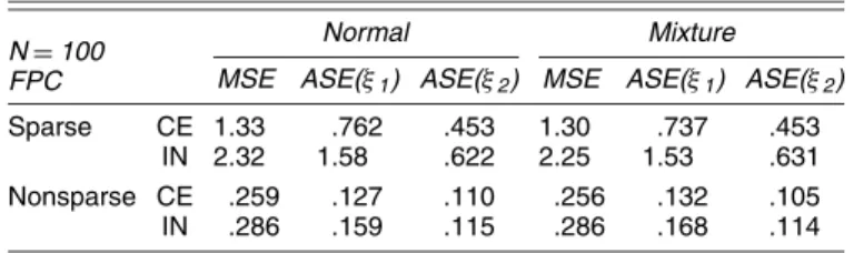
To demonstrate the superior performance of the conditional method, Table 1 reports the average mean squared error (MSE) for the true curves Xi, MSE=ni=1
10
0 {Xi(t)−XiK(t)}2dt/n, whereXiK(t)= ˆµ(t)+Kk=1ξˆikφˆk(t) and the ξˆik’s were ob-tained using either the proposed PACE method (5) or the in-tegration method. The number of eigenfunctions K in each run was chosen by the AIC (11). In each simulation consisting of 100 Monte Carlo runs (for a total of 400 runs, normal/mixture and sparse/nonsparse), there were always more than 95 runs in which two eigenfunctions were chosen.
Another outcome measure of interest is the average squared error (ASE) for the two FPC scores, ASE(ξk)=
n i=1(ξˆik− ξik)2/n, k=1,2, also listed in Table 1. We also compared the two methods for irregular but nonsparse simulated data, where the number of observations for each curve was randomly cho-sen from {30, . . . ,40}, with results given in Table 1. We find that the gains in the sparse situation are dramatic when switch-ing from the traditional method to the PACE method. For the case of an underlying normal distribution, the MSE was re-duced by 43% using the PACE method (5) as compared with
Table 1. Results for FPC Analysis Using Conditional Expectation (CE, corresponding to PACE) and Integration (IN) Methods for 100 Monte Carlo Runs With N=100 Random Trajectories per Sample,
Generated With Two Random Components N=100
FPC
Normal Mixture MSE ASE(ξ1) ASE(ξ2) MSE ASE(ξ1) ASE(ξ2) Sparse CE 1.33 .762 .453 1.30 .737 .453
IN 2.32 1.58 .622 2.25 1.53 .631 Nonsparse CE .259 .127 .110 .256 .132 .105 IN .286 .159 .115 .286 .168 .114 NOTE: Shown are the averages of estimated mean squared prediction error, MSE, and average squared error, ASE(ξk),k=1, 2, as described in Section 4. The number of components for each Monte Carlo run is chosen by the AIC criterion (11).
the traditional method; the ASE(ξk)were reduced by 52%/27% (k=1,2). For the mixture distribution case, the decreases were still 42% for MSE and 52%/28% for ASE(ξk) (k=1,2). In nonsparse situations, the traditional estimates provide reason-able approximations to the underlying integrals, but neverthe-less PACE still produces better estimates, with improvements of 10%/10% for MSE and 20%/21%,5%/8% for ASE(ξk), k=1,2, for normal/nonnormal samples. We conclude that the gains obtainable using PACE are substantial for sparse data and also extend to the case of dense and non-Gaussian data.
5. APPLICATIONS 5.1 Longitudinal CD4 Counts
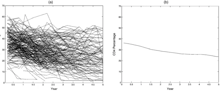
Because CD4 counts constitute a critical assessment of the status of the immune system and are used as an important marker in describing the progress to AIDS in adults, CD4 cell counts and CD4 percentages (i.e., CD4 counts divided by the to-tal number of lymphocytes) are commonly used markers for the health status of human immunodeficiency virus (HIV) infected persons. The dataset considered here is from the Multicenter AIDS Cohort Study, which includes repeated measurements of physical exams, laboratory results, and CD4 percentages for 283 homosexual men who became HIV-positive between 1984 and 1991. All individuals were scheduled to have their measurements made at semiannual visits. However, because many individuals missed scheduled visits and the HIV infec-tions happened randomly during the study, the data are sparse, with unequal numbers of repeated measurements per subject and different measurement times, Tij, per individual. The num-ber of observations per subject ranged from 1 to 14, with a median of 6. The trajectories in their entirety are assembled in Figure 1(a).
That the data from such a classical longitudinal study, with measurements intended to be spaced at regular 6-month inter-vals, are quite well suited for analysis by PACE is illustrated by Figure 2. As this figure shows, the assembled pairs(Tij,Tik)are sufficiently dense in the domain plane, and estimation of the co-variance function (A.2) is feasible for these data. Further details
Figure 2. Assembled Pairs (Tij,Tik) of All Subjects, i=1, . . . , n,
j, k=1, . . . , Ni, for the CD4 Count Data. Although the data available per
subject are sparse, the assembled data fill the domain of the covariance surface quite densely.
about design, methods, and medical implications of the study were given by Kaslow et al. (1987). Fan and Zhang (2000) and Wu and Chiang (2000) analyzed these data with varying coef-ficient models adapted to longitudinal data, and Diggle, Liang, and Zeger (1994) discussed classical longitudinal approaches for these data.
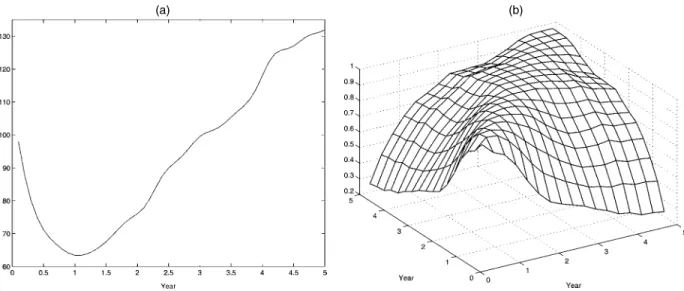
The objectives of our analysis are to estimate the overall trend over time, uncover subject-specific variation patterns, ex-tract the dominant modes of variation, and recover individual trajectories from sparse measurements. This includes predict-ing the time course for an individual given only few observa-tions, and constructing pointwise and simultaneous bands for an individual’s trajectory. The estimate of the mean function using local linear smoothing is shown in Figure 1(b), revealing the overall decreasing trend in CD4 cell counts. Estimates of variance and correlation functions are shown in Figure 3; the variance is clearly nonstationary, with high variability at very
(a) (b)
(a) (b)
Figure 3. (a) Smooth Estimate of the Variance Function for CD4 Count Data and (b) Smooth Estimate of the Correlation Function, Eliminating the “Raw” Data Falling on the Diagonal.
early times, decreasing until about 1 year and then increasing again. Measurements made on the same subject are strongly correlated, irrespective of the time difference. However, the cor-relation between very early and late counts dies off relatively rapidly, whereas for middle and later times, the dependence pat-terns persist more strongly. These features would be difficult to anticipate in a traditional parametric model; they would not be produced, by, for example, linear random-effects models.
Next, consider the eigenfunction decomposition of the esti-mated covariance surface. Three eigenfunctions shown in the upper panels of Figure 4 are used to approximate the infinite-dimensional process. The choice K=3 emerges as a reasonable choice, supported both by the AIC (11) and one-curve-leave-out cross-validation. The first eigenfunction is somewhat similar to the mean function, the second corresponds to a contrast
be-Figure 4. Smooth Estimates of the First Three Eigenfunctions for CD4 Count Data (top panels) and Observations (circles) and Predicted Trajectories (dashed lines) for the Three Individuals With the Largest Projections on the Respective Eigenfunctions Above, Overlaid With the Overall Estimated Mean Function (solid lines) (bottom panels).
tween very early and very late times, and the third corresponds to a contrast between the early and the medium plus later times. These eigenfunctions account for 76.9%, 12.3%, and 8.1% of the total variation. Most of the variability is thus in the direc-tion of overall CD4 percentage level. In exploring such data, extreme individual cases are difficult to detect by visual exami-nation due to irregular sampling and substantial noise. One way to explore the variability in the sample and to single out extreme cases is to identify cases that exhibit large principal component scores in the directions of a few leading eigenfunctions (Jones and Rice 1992). Three such cases, corresponding to the largest absolute values of the projections on the first three eigenfunc-tions, are shown in the lower panels of Figure 4.
The predicted curves and 95% pointwise and simultaneous confidence bands for four randomly chosen individuals are dis-played in Figure 5, where the principal component scores of
Figure 5. Observations (circles), Predicted (solid lines) Trajectories, and 95% Pointwise (dashed lines) and Simultaneous (dotted lines) Bands for Four Randomly Chosen Individuals, for the CD4 Count Data.
each subject are estimated using the PACE method. The pre-dicted curves are seen to be reasonably close to the obser-vations. Even for individuals with very sparse measurements, one is still able to effectively recover their random trajecto-ries, combining the information from that individual and the entire collection. For example, the PACE principle of borrow-ing strength from the entire sample for predictborrow-ing individual trajectories makes it feasible to predict trajectories and con-struct corresponding prediction bands for those cases where only one observation available per subject, as exemplified in the lower left panel of Figure 5. The predictions based on only one observation per subject work reasonably well, as is demon-strated in the second example described in Section 5.2 (see the lower right panel in Fig. 9, where only one single measurement enclosed in the circle is used for the prediction of the trajec-tory). Because we need to be able to consistently estimate the covariance structure, it is, however, not feasible to apply the method if there is only one observation available per subject for all subjects. Note that the 95% simultaneous bands show a widening near the endpoints due to end effects and increased variance near the ends, and that all observed data fall within these bands.
5.2 Yeast Cell Cycle Gene Expression Profiles
Time-course gene expression data (factor-synchronized) for the yeast cell cycle were obtained by Spellman et al. (1998). The experiment started with a collection of yeast cells, whose cycles were synchronized (α factor-based) by a chemical process. There are 6,178 genes in total, and each gene ex-pression profile consists of 18 data points, measured every 7 minutes between 0 and 119 minutes, covering two cell cy-cles. Of these genes, 92 had sufficient data and were identified by traditional methods, of which 43 are related to G1 phase regulation and 49 are related to non-G1 phase regulation (i.e., S, S/G2, G2/M, and M/G1 phases) of the yeast cell cycle; these genes serve as a training set. The gene expression level mea-surement at each time point is obtained as a logarithm of the expression-level ratio.
To demonstrate the usefulness of the PACE method for sparse functional data, we artificially “sparsify” the measurements made for the genes in the training data, then compare the results obtained from this “sparsified” data with those obtained from the complete data. To sparsify the expression measurements made for the ith gene expression profile, the number of mea-surements Ni is randomly chosen between 1 and 6 with equal probability, and the measurement locations are then randomly selected from the 18 recorded gene expression measurements per profile. The median number of observations per gene ex-pression profile for the resulting sparse data is just 3.
Analyses of both complete and sparsified yeast cell cycle pro-file data are illustrated in Figures 6–8. The two mean function estimates for the sparse and complete data, obtained by local linear smoothing of the pooled data, are close to each other and demonstrate periodicity [see Fig. 8(a), presenting two cell cy-cles]. The two smooth covariance surface estimates revealing the structure of the underlying process are displayed in Fig-ure 7. Both surfaces are very similar and exhibit periodic fea-tures. We use the first two eigenfunctions to approximate the
(a) (b)
Figure 6. Complete Measurements (a) of Gene Expression Profiles and a Randomly “Sparsified” Subset (b) for 92 Yeast Cell Cycles.
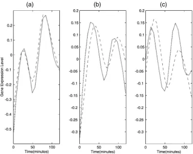
expression profiles [Figs. 8(a) and 8(c)]. The estimates of the first two eigenfunctions obtained from both sparse and com-plete data are also close and reflect periodicity, explaining ap-proximately 75% of the total variation.
We randomly select four genes, and present the predicted profiles obtained from both sparse and complete data and the confidence bands using only the sparse data in Figure 9. We note that the trajectories obtained for the complete data are en-closed in the simultaneous 95% confidence bands constructed from the sparse data. The predictions obtained from the sparse data are similar to those constructed from the complete data and are reasonable when compared with the complete measure-ments. This demonstrates that the PACE method allows us to effectively recover entire individual trajectories from fragmen-tal data.
(a) (b)
Figure 7. Smooth Surface EstimatesG (A.2) of the Covariance Func- tions Obtained From the Complete Data (a) and From the Sparsified Data (b) for Yeast Cell Cycle Gene Expression Profiles.
(a) (b) (c)
Figure 8. Smooth Estimates of the Mean Function (a), the First (b) and Second (c) Eigenfunctions, Obtained From Sparse (solid lines) and Complete (dashed lines) Gene Expression Data.
6. CONCLUDING REMARKS
Besides the general application to FPC analysis for sparse and irregular data, an application of our proposed PACE method to impute missing data in longitudinal studies is also feasible. Consider a regular design where for some subjects many data are missing. The PACE method can then be used to impute the missing data from predicted trajectories.
An interesting finding from the simulation study is that the PACE method improves on traditional FPC analysis even under dense and regular designs. This improvement is due to replacing integrals by conditional expectations when determining FPC scores. The conditioning step can be interpreted as shrinkage
Figure 9. Predicted Gene Expression Profiles Obtained From Com-plete Measurements (thick solid lines) and From Sparse Measure-ments (solid lines) for Four Randomly Selected Genes. Also shown are 95% pointwise (dashed lines) and simultaneous (dotted lines) bands ob-tained exclusively from the sparse data. Solid circles indicate the mea-surements for the complete data, and solid circles enclosed by an open circle correspond to the randomly sampled sparse data.
of these random effects toward 0. The observed improvement indicates that PACE can also be used to advantage for regularly spaced data, which enhances this method’s appeal. We conclude that the underlying principle of borrowing strength from an en-tire sample of curves to predict individual trajectories shows promise in applications.
APPENDIX: PROOFS AND AUXILIARY RESULTS We assume regularity conditions for the marginal and joint densities
f(t), g(t,y), and g2(t1,t2,y1,y2). Letν1, ν2, andbe given integers, with 0≤ν1+ν2< . Then the following conditions apply:
(B1.1) (d/dt)f(t) exists and is continuous onT with f(t) >0 onT.
(B1.2) (d/dt)g(t,y)exists and is uniformly continuous onT× . (B1.3) (d/(dt1
1 dt 2
2 ))g2(t1,t2,y1,y2) exists and is uniformly
continuous onT2× 2, for1+2=,0≤1, 2≤.
The assumptions for kernel functionsκ1: → andκ2: 2→
are as follows. We say that a bivariate kernel functionκ2is of order
(ν, ), whereνis a multi-indexν=(ν1, ν2), if u1v2κ 2(u,v)du dv = 0, 0≤1+2< , 1=ν1, 2=ν2 (−1)|ν||ν|!, 1=ν1, 2=ν2 =0, 1+2=, (A.1)
where|ν| =ν1+ν2. A univariate kernelκ1is of order(ν, )for a
uni-variateν=ν1, if (A.1) holds with2=0 on the right side, integrating only over the argument u on the left side.
(B2.1a) κ1is compactly supported,κ12=
κ12(u)du<∞. (B2.2a) κ1is a kernel function of order(ν, ).
(B2.1b) κ2 is compactly supported, κ22 = κ22(u,v) ×
du dv<∞.
(B2.2b) κ2is a kernel function of order(ν, ).
We define the local linear scatterplot smoother forµ(t)by minimiz-ing n i=1 Ni j=1 κ1 Tij−t hµ {Yij−β0−β1(t−Tij)}2 (A.2)
with respect toβ0andβ1. The estimate ofµ(t)is thenµ(ˆ t)= ˆβ0(t). The local linear surface smoother for G(s,t)is defined by minimizing
n i=1 1≤j=l≤Ni κ2 Tij−s hG ,Til−t hG ×Gi(Tij,Til)−f β, (s,t), (Tij,Til) 2 , (A.3)
where f(β, (s,t), (Tij,Til))=β0+β11(s−Tij)+β12(t−Til).
Min-imization is with regard toβ=(β0, β11, β12), yielding the estimate
G(s,t)= ˆβ0(s,t). To obtain the adjusted estimate of G(s,t)on the di-agonal [i.e.,G(t)], we first rotate both the x-axis and y-axis by 45 de-grees clockwise and obtain the coordinates of(Tij,Tik)in the rotated
axes, denoted by(Tij∗,Tik∗), that is, T∗ ij Tik∗ =−√√2/2 √2/2 2/2 √2/2 T ij Tik . We then define the surface estimateG¯(s,t)by minimizing the weighted least squares, n i=1 1≤j=l≤Ni κ2 T∗ ij−s hG ,T ∗ il−t hG ×Gi(Tij∗,Til∗)−g γ, (s,t), (Tij∗,Til∗)2, (A.4)
where g(γ, (s,t), (Tij∗,Til∗))=γ0+γ1(s−Tij∗)+γ2(t−Tik∗)2.
Min-imization is with respect toγ =(γ1, γ2, γ3)T, leading to G¯(s,t)=
ˆ
γ0(s,t). Because of the rotation, the estimate of the covariance sur-face on the diagonal,G(t), is now indeedG¯(0,t/√2), obtained with the rotated coordinates.
The following auxiliary results provide the weak uniform con-vergence rate for univariate weighted averages defined later (cf.
Bhattacharya and Müller 1993). For a positive integer l≥1, let
(ψp)p=1,...,l be a collection of real functionsψp: 2→ , that
sat-isfy the following conditions:
(C1.1a) ψpare uniformly continuous onT × .
(C1.2a) The functions (d/dt)ψp(t,y) exist for all arguments (t,y)and are uniformly continuous onT × .
(C1.3a) ψp2(t,y)g(t,y)dy dt<∞.
Bandwidths hµ=hµ(n)used for one-dimensional smoothers are
as-sumed to satisfy the following:
(C2.1a) hµ→0,nhνµ+1→ ∞, nh2µ+2<∞, as n→ ∞.
Define the weighted averages
pn=pn(t) = 1 nhνµ+1 n i=1 1 EN Ni j=1 ψp(Tij,Yij)κ1 t−Tij hµ , p=1, . . . ,l,
and the quantity
µp=µp(t)
= dν
dtν
ψp(t,y)g(t,y)dy, p=1, . . . ,l.
Lemma A.1. Under (A1.1), (A1.2), (A3.1), (B1.1), (B1.2), (B2.1a),
(B2.2a), (C1.1a)–(C1.3a), and C(2.1a),τpn=supt∈T |pn−µp| = Op(1/(√nhνµ+1)).
Proof. Note that E|τpn| ≤supt|Epn − µp| +E{supt|pn − Epn|}, where t takes values inT and E|τpn| =O(1/(√nhνµ+1))
im-plies thatτpn=Op(1/(√nhνµ+1)).
Using a Taylor expansion to order, it is easy to show that Epn= µp+O(hµ−ν),where the remainder term is uniform in t, observing that(d/dt)ψp(t,y)and(d/dt)g(t,y)are uniformly continuous. It remains to show that E{supt|pn−Epn|} =O(1/(√nhνµ+1)).
Re-call that the inverse Fourier transform isζ1(t)=
e−iutκ1(u)du. We may insertκ1((t−Tij)/hµ)= eiv(t−Tij)/hµζ 1(v)dv/(2π )intopn. Letting ϕpn(u)= 1 n n l=1 1 EN Nl j=1 eiuTljψ p(Tlj,Ylj), we obtain pn= 1 nhνµ+1 n l=1 1 EN Nl j=1 κ1 t−T lj hµ ψp(Tlj,Ylj) = 1 2πhνµ ϕpn(u)e−ituζ1(uhµ)du, and thus sup t | pn−Epn| ≤ 1 2πhνµ |ϕpn(u)−Eϕpn(u)| · |ζ1(uhµ)|du.
Note that E|ϕpn(u)−Eϕpn(u)| ≤ E[ϕpn(u)−Eϕpn(u)]2, and
be-cause{Ti,Yi,Ni}are iid, using the Cauchy–Schwarz inequality,
var(ϕpn(u))=1 nvar 1 EN N j=1 eiuTjψp(T j,Yj) ≤1 nE 1 EN N j=1 eiuTjψ p(Tj,Yj) 2 ≤1 nE 1 (EN)2 N j=1 ei2uTj N j=1 ψp2(Tj,Yj) ≤1 nE N (EN)2 N j=1 Eψp2(Tj,Yj)|N =1 nEψ 2 p(T,Y), implying that E sup t |pn−Epn| ≤ 1 2πhνµ E{|ϕpn(u)−Eϕpn(u)|} · |ζ1(uhµ)|du ≤ Eψ2 p(T,Y) |ζ1(u)|du 2π 1 √ nhνµ+1 .
Because nh2µ+2<∞implies that hµ−ν=O(1/(√nhνµ+1)), the result follows.
Analogous to Lemma A.1, we obtain the rate of uniform conver-gence in the two-dimensional situation. Let{θp(t,s,y1,y2)}p=1,...,lbe
a collection of real functionsθp: 4→ with the following
proper-ties:
(C1.1b) θpare uniformly continuous onT2× 2. (C1.2b) The functions (d/(dt1ds2))θp(t,s,y
1,y2) exist for all
arguments(t,s,y1,y2)and are uniformly continuous on T2× 2, for
1+2=,0≤1, 2≤.
(C1.3b) θp2(t,s,y1,y2)g2(t,s,y1,y2)dy1dy2dt ds<∞.
The sequence of bandwidths hG =hG(n) for the two-dimensional
smoothers satisfies the following:
(C2.1b) hG→0,nh|Gν|+2→ ∞, nh2G+4<∞, as n→ ∞.
Define the weighted averages,
pn=pn(t,s) = 1 nh|Gν|+2 n i=1 1 EN(EN−1) × 1≤j=k≤Ni θp(Tij,Tik,Yij,Yik)κ2 t−Tij hG ,s−Tik hG and p=p(t,s) = 1+2=|ν| d|ν| dt1ds2 × θp(t,s,y1,y2)g2(t,s,y1,y2)dy1dy2, p=1, . . . ,l. Lemma A.2. Under (A1.1), (A1.2), (A3.2), (B1.1b), (B1.2b),
(B2.1)–(B2.3), (C1.1b)–(C1.3b), and C(2.1b),ϑpn=supt,s∈T|pn− p| =Op(1/(√nh|ν|+2)).