econstor
www.econstor.eu
Der Open-Access-Publikationsserver der ZBW – Leibniz-Informationszentrum Wirtschaft
The Open Access Publication Server of the ZBW – Leibniz Information Centre for Economics
Nutzungsbedingungen:
Die ZBW räumt Ihnen als Nutzerin/Nutzer das unentgeltliche, räumlich unbeschränkte und zeitlich auf die Dauer des Schutzrechts beschränkte einfache Recht ein, das ausgewählte Werk im Rahmen der unter
→ http://www.econstor.eu/dspace/Nutzungsbedingungen nachzulesenden vollständigen Nutzungsbedingungen zu vervielfältigen, mit denen die Nutzerin/der Nutzer sich durch die erste Nutzung einverstanden erklärt.
Terms of use:
The ZBW grants you, the user, the non-exclusive right to use the selected work free of charge, territorially unrestricted and within the time limit of the term of the property rights according to the terms specified at
→ http://www.econstor.eu/dspace/Nutzungsbedingungen By the first use of the selected work the user agrees and declares to comply with these terms of use.
Kleppe, Tore Selland; Liesenfeld, Roman
Working Paper
Efficient high-dimensional importance
sampling in mixture frameworks
Economics working paper / Christian-Albrechts-Universität Kiel, Department of Economics,
No. 2011,11
Provided in cooperation with:
Christian-Albrechts-Universität Kiel (CAU)
Suggested citation: Kleppe, Tore Selland; Liesenfeld, Roman (2011) : Efficient high-dimensional
importance sampling in mixture frameworks, Economics working paper /
Christian-Albrechts-Universität Kiel, Department of Economics, No. 2011,11, http://hdl.handle.net/10419/53125
efficient high-dimensional importance
sampling in mixture frameworks
by Tore Selland Kleppe and Roman Liesenfeld
No 2011-11Ecient high-dimensional importance sampling
in mixture frameworks
Tore Selland Kleppe
∗Roman Liesenfeld
†June 8, 2011
Abstract
This paper provides high-dimensional and exible importance sam-pling procedures for the likelihood evaluation of dynamic latent variable models involving nite or innite mixtures leading to possibly heavy tailed and/or multi-modal target densities. Our approach is based upon the ef-cient importance sampling (EIS) approach of Richard and Zhang (2007) and exploits the mixture structure of the model when constructing impor-tance sampling distributions as mixture of distributions. The proposed mixture EIS procedures are illustrated with ML estimation of a student-t
state space model for realized volatilities and a stochastic volatility model with leverage eects and jumps for asset returns.
Keywords: Dynamic latent variable model; Importance sampling; Marginalized likelihood; Mixture; Monte Carlo; Realized Volatility; Stochas-tic volatility.
JEL classication codes: C15
∗Department of Mathematics, University of Bergen, Bergen, Norway, (Corresponding
au-thor, email: [email protected], phone: +4795922364, fax: +4755589672, address: Uni-versitetet i Bergen, Matematisk institutt, Postboks 7803, 5020 Bergen, Norway)
1 Introduction
In recent decades Monte Carlo (MC) procedures based upon Importance Sampling (IS) have been successfully applied for the analysis of econo-metric models involving multiple integrals for which no analytical solu-tions exist. Important applicasolu-tions of IS are the evaluation of Bayesian a-posteriori expectations of functions of parameters of interest and that of likelihood functions in the presence of unobservable latent variables see, e.g., Kloek and Dijk (1978); Geweke (1989); Durbin and Koopman (1997).
It is well-known that the reliable and ecient use of IS requires that the IS auxiliary density closely mimics the target density kernel which needs to be integrated, and exhibits tails that do not decay more quickly than the tails of the target density (see, Geweke (1989); Robert and Casella (2004)). This implies that IS implementations have to be tailored to the problem under consideration which has proved to be a signicant obstacle to routine applications of IS. This is especially true for applications with ill behaved, and therefore, dicult to approximate target densities. A survey of IS approaches is found, e.g., in Liesenfeld and Richard (2001).
Another critical issue is that most of the existing IS approaches do not appear to be applicable to highly multidimensional integration problems. Prominent exceptions are the high-dimensional IS methods proposed by Shephard and Pitt (1997); Durbin and Koopman (1997, 2000), and the Ecient Importance Sampling (EIS) procedure of Richard and Zhang (2007). Existing implementations of those methods rely on IS densities from the exponential family of distributions, which, in the case of EIS, considerably simplies the implementation. While the IS approaches of Shephard and Pitt (1997) and Durbin and Koopman (1997, 2000) use Gaussian IS densities constructed from local Taylor-series approximations to the target density, the IS densities of the EIS approach of Richard and
Zhang (2007) are based upon global approximations to the target obtained via a sequence of low-dimensional auxiliary least-squares regressions.
Those high-dimensional IS approaches have been successfully applied for the computation of the likelihood for a broad range of dynamic latent variable (DLV) models, where the target densities are reasonably well be-haved such that they can be well approximated by IS densities from the exponential family of distributions (see, e.g., Sandmann and Koopman (1998); Liesenfeld and Richard (2003, 2010); Bauwens and Galli (2009)). However, for DLV models with pathological target densities, featuring e.g. multi-modality and/or fat tails, those high-dimensional procedures based upon IS densities from the exponential family might have severe conver-gence problems. In the context of DLV models, such ill-behaved tar-get densities are often caused by nite or innite mixture-of-distributions specications assumed for some of the variables. Examples, to be dis-cussed further below are diusion models for stock prices with discrete jumps and state space models with student-tmeasurement errors. Hence,
there exists a need for high-dimensional IS procedures based upon exible IS densities beyond the exponential family of distributions.
In the present paper, we extend the high-dimensional EIS approach of Richard and Zhang (2007), by introducing nite and innite mixture of distributions as exible classes of IS distributions allowing to approximate target densities which are possibly heavy-tailed and/or multi-modal. Our approach is particularly well adapted to the likelihood evaluations for DLV models involving variables characterized by a mixture of distribu-tions, which can be exploited when constructing the IS densities. Under appropriate simplifying conditions our proposed mixture EIS procedures rely, similarly to EIS implementations for IS densities from the exponen-tial family, on a simple sequence of auxiliary least-squares regressions used to obtain close approximations to the integrand.
densities are the `split'-Student IS approach of Geweke (1989), the `defen-sive' mixture technique proposed by Hesterberg (1995) and the adaptive method of Ardia et al. (2009) using mixture of Student-t distributions. While those approaches have been successfully applied to lower dimen-sional Bayesian integration problems, they do not appear to be applicable to very high-dimensional integrals, which needs to be approximated, e.g., for the likelihood evaluation of DLV models.
The rest of the paper is organized as follows. In Section 2, we briey review the generic principles of EIS, and in Section 3 we introduce mixture EIS approaches based upon nite and innite mixtures of distributions. Section 3 also provides two simple one-dimensional examples illustrat-ing the benets of the proposed mixture EIS procedures. Sequential im-plementation of mixture EIS procedures for high-dimensional integration required for a likelihood analysis of realistic models is illustrated in Sec-tion 4. In particular, we discuss the ML estimaSec-tion of a student-t state
space model for realized volatilities (Section 4.1) and a stochastic volatil-ity model with a jump component for asset returns (Section 4.2). Section 5 concludes.
2 Ecient importance sampling (EIS)
2.1 General principle
Consider the problem of evaluating an integral of the form
I=
Z
ϕ(z)dz, (1)
where ϕ : ∆ 7→ R+ with ∆ ⊆ RT. Of special interest in this paper focusing on likelihood evaluations of DLV models is the case where the econometric model under consideration leads to an initial factorization of
the integrand of the form
ϕ(z) =g(z)·p(z), (2)
wherepis a probability density function forz referred to as the initial or
natural (model based) sampler, andg: ∆7→R+is ap-integrable function. IS integration consists of selecting an IS density, saym(z), and
rewrit-ing Equation (1) as I= Z ϕ(z) m(z) ·m(z)dz. (3)
The corresponding MC IS estimator ofI is then given by
ˆ I= 1 M M X j=1 ϕ(z(j)) m(z(j)), (4)
where {z(j), j = 1, ..., M} denotes a set of M identically independently
distributed draws fromm.
The technical conditions, under which the IS estimator (4) converges almost surely toIand its variance is nite are discussed in Geweke (1989)
and Robert and Casella (2004). A sucient condition for the niteness the variance ofIˆis that|ϕ(z)/m(z)|be bounded above on∆.
Ecient IS algorithms are those for which the variance ofIˆis as small
as possible. This suggests to select an IS density m, which mimics the
target integrandϕ(z) as close as possible such that the ratioϕ(z)/m(z)
is almost constant on∆. The EIS approach of Richard and Zhang (2007)
provides an algorithm to select such an ecient sampler within a prese-lected parametric class of densities, say M={m(z;a), a∈ A}, indexed
by the auxiliary parametera. For lower dimensional problems, it
approxi-mates the targetϕ(z)by the density kernelk(z, a)associated with density
m(z;a), where the correspondence between kandmis given by
m(z;a) = k(z, a)
χ(a) with χ(a) =
Z
The near optimal value aˆ obtains as the solution to the least-squares problem {ˆa,cˆ}=argmin a,c Z [lnϕ(z)−c−lnk(z, a)]2m(z;a)dz, (6)
wherecrepresents an intercept meant to calibrate the log-ratioln(ϕ/k).
Since the IS sampling densitymitself depends upona, the optimization
problem (6) is reinterpreted as the search for a xed-point solution with an operational MC version based upon the following step-wise recursion: Givenˆa(`)∈A, generate intermediate draws{z(j,`), j= 1, ..., M}from the step-`EIS samplerm(z; ˆa(`))and solve
{ˆa(`+1),cˆ(`+1)}=argmin a,c M X j=1 h lnϕ(z(j,`))−c−lnk(z(j,`), a)i 2 . (7)
At convergence, wherebyaˆ' ˆa(`+1) 'aˆ(`), the density m(z; ˆa) is used
to compute the EIS estimate ofI according to Equation (4). An initial
valueˆa(0) can be obtained by a local approximation ofϕor by the value
of a associated with the natural sampler p. In order to secure smooth
convergence to a xed-point solution, all draws{z(j,`)}must be obtained
by transformation of a set of Common Random Numbers (CRNs){u(j)}
from a canonical distribution associated withM, i.e. one that does not dependent ona(e.g. a standardized Normal, whenmis Gaussian).
Although the EIS approach is not restricted to any particular family of IS densitiesm, its existing implementations typically rely upon
densi-ties from the exponential family. In this case, the log kernellnk can be
parameterized in such a way that it is linear in the auxiliary parameter
aand the minimization problem (7) reduces to a computationally simple
linear LS problem. If, in addition, the initial sampler p belongs to the
exponential family andMis selected to be a parametric class containing
pas a particular member, one can exploit the property of the exponential
allows one to dene the EIS density kernelkas
k(z, a) =p(z)ζ(z, a), (8)
whereζ(z, a) is itself a density kernel associated withm(for details, see
Richard and Zhang (2007)). It follows that p(z) cancels out in the
re-gression (7) which simplies into a rere-gression oflng(x)on a constant and lnζ(z, a).
2.2 Sequential high-dimensional EIS
High-dimensional EIS used, e.g., for the likelihood evaluation of DLV mod-els, requires that the integrandϕ(z) =g(z)p(z)in Equations (1) and (2)
as well as the EIS densitym(z;a)be factorized into low-dimensional
com-ponents in accordance with a natural pre-ordering partition ofz obtained
from the model specication, say z1, ..., zT, with an initial conditionz0.
The factorizations ofϕandmconformably withzare
ϕ(z) = T Y t=0 ϕt(z(t)) =p0(z0) T Y t=1 gt(z(t))pt(zt|z(t−1)), (9) m(z;a) = T Y t=0 mt(zt|z(t−1);at), (10) wherez(t)= (z0, ..., zt),a= (a0, ..., aT)andmt(z0|z(−1);a0) =m0(z0;a0).
The natural model based sampling density of z is the product p(z) =
p0(z0) QTt=1pt(zt|z(t−1)). Denoting the approximating kernel of the IS
densitymt(zt|z(t−1);at)bykt(z(t), at), with mt(zt|z(t−1);at) = kt(z(t), at) χt(z(t−1), at) , and (11) χt(z(t−1), at) = Z kt(z(t), at)dzt,
the integral to be approximated can be rewritten as I=χ0(a0) Z h T Y t=0 ϕt(z(t))χt+1(z(t), at+1) kt(z(t), at) iYT t=0 mt(zt|z(t−1);at)dz(T), (12) whereχT+1(·)≡1.
EIS then aims at selecting values of the auxiliary parameters {at}
that minimize factor by factor the variance of the ratiosϕt·χt+1/kt as
functions of z(t) with respect to the mt-distributions. An operational
MC version of that xed-point minimization problem generates at step`
intermediate draws {z(tj,`)t = 0, ..., T;j = 1, ..., M}from the step-` EIS
sampler m(z; ˆa(`)) and solves back recursively the following sequence of
T+ 1least-squares problems {ˆa(t`+1),ˆc (`+1) t }=argmin at,ct M X j=1 h lnϕt(z((tj,`)))χt+1(z((j,`t)),ˆa(t`+1+1)) (13) −ct−lnkt(z((tj,`)), at) i2 , t=T, T −1, ...,0.
The corresponding MC-EIS estimate of the integralI is given by
ˆ I=χ0(α0) 1 M M X j=1 hYT t=0 ϕt(z((tj)))χt+1(z((tj)),ˆat+1) kt(z (j) (t),ˆat) i , (14)
where {zt(j), t = 0, ..., T, j = 1, ..., M} are draws from the EIS density
m(z; ˆa).
This sequential high-dimensional EIS approach has been successfully applied for likelihood evaluations for DLV models, where the natural sam-pling densitiesptin Equation (9) belong to the exponential family and the
gts are well-behaved functions inzt. In this case,ϕtχt+1 can be
reason-ably well approximated by exponential family density kernelskt obtained
as parametric extensions of the natural samplerptaccording to Equation
(8). As mentioned above, the use of EIS densities from the exponential family considerably reduces the computational eort and simplies the
implementation of EIS by reducing it to the solution of linear LS prob-lems. Since the number of auxiliary LS problems is proportional to the dimension of the integral, this linearity becomes particularly desirable for very high-dimensional integration (1000+).
Applications of EIS in such well-behaved frameworks include the com-putation of the likelihood and ML estimates for stochastic volatility mod-els (Liesenfeld and Richard (2003); Kleppe et al. (2010)), stochastic con-ditional intensity processes (Bauwens and Galli (2009)), multinomial-multiperiod Probit models (Liesenfeld and Richard (2010)) and dynamic factor models for multivariate count data (Jung et al. (2011)).
In many practical applications, however, DLV model specications with natural sampling densities p within the exponential family appear
to be too restrictive calling for more exible alternatives. A straightfor-ward extension of simple distributions from the exponential family is the class of mixture distributions providing a exible environment for econo-metric modeling which enjoys great popularity. However, DLV models with natural sampling distributionspassumed to be nite or innite
mix-tures of distributions lead to possibly multi-modality and/or fat tailed targetsϕ. In such cases, the performance of (E)IS based upon sampling
densitiesmfrom the exponential family might be seriously hampered by
a large or even innite variance of the IS estimatorIˆresulting from poor
global approximations ofϕby exponential density kernelsk.
In the following section, we present algorithms to construct exible EIS densities for nite and innite mixture frameworks generating pos-sibly ill-behaved target integrands. The proposed algorithms exploit the mixture specication of the target density and use a data-augmentation step demarginalizing the mixture density to include the mixing variable as an additional latent variable. As we shall illustrate below, this articial extension of the space of integration typically leads to better behaved tar-get integrands (for the extended space), which can be well approximated
by standard distributions belonging to the exponential family.
3 EIS in mixture frameworks
In this section we introduce EIS in innite mixture (subsection 3.1) as well as in nite mixture frameworks (subsection 3.2) focusing on simple one-dimensional integration problems. This provides a convenient setting to discuss and illustrate the key features of mixture EIS. Sequential imple-mentations for high-dimensional integration required to analyze realistic models, will be discussed in Section 4.
3.1 Innite mixture EIS
Assume that the natural sampling density of the integral given by Equa-tions (1) and (2) can be represented as an innite mixture specication of the form
p(z) =
Z
p(z|w)p(w)dw, (15)
wherep(z|w)is a conditional density depending on a latent auxiliary
vari-ablew with density p(w), referred to as the mixing density. Prominent
examples for innite mixture density functions include the student-tand
the negative binomial density.
Such a representation of the natural sampling density allows us to write the integral (1) as
I=
Z
g(z)p(z|w)p(w)dwdz. (16)
Based upon this demarginalization which extends the space of integra-tion, EIS can be implemented using a joint IS density for the augmented set of variables, say m(z, w;a), and exploiting the factorization of the
natural sampler given byp(z|w)p(w). The factorization of the joint IS
m(z|w;az)m(w;aw), with m(z|w;az) = k(z, w;az) χ(w, az) , m(w;aw) = k(w;aw) χ(aw) , (17)
where theks andχs are the approximating EIS density kernels and the
corresponding integrating factors, respectively. This allows us to rewrite the integral (16) as I=χ(aw) Z h g(z)p(z|w) k(z, w;az) ihχ(w, az)p(w) k(w;aw) i m(z, w;a)dwdz. (18)
Then the EIS values of the auxiliary parameters, ˆa = (ˆa(z`+1),aˆ
(`+1)
w ),
obtain from the recursive solution of the following two LS problems
min az,cz M X j=1 h ln[g(z(j,`))p(z(j,`)|w(j,`))]−cz−lnk(z(j,`), w(j,`), az) i2 min aw,cw M X j=1 h ln[χ(w(j,`),aˆ(z`+1))p(w (j,`) )]−cw−lnk(w(j,`), aw) i2 ,(19)
where {(z(j,`), w(j,`)), j= 1, ..., M}are draws from the step-`
intermedi-ate samplerm(z, w; ˆa(`)). The nal EIS MC estimate of the augmented
integral is then given by
ˆ I= 1 M m X i=1 g(z(j))p(z(j)|w(j))p(w(j)) m(z(j), w(j); ˆa) , (20)
where(z(j), w(j))represent draws from the nal joint EIS sampler.
Hence, if bothg(z)p(z|w)andχ(w,·)p(w)can be reasonably well
ap-proximated by density kernels from the exponential family, this approach allows us to retain the linearity of the EIS approximation problem, even for integrands ϕ(z) which are generated by innite mixtures, and which
cannot be well approximated by a univariate IS sampling density for z
from the exponential family.
At a rst glance, extending the dimension of integration seems to be counterintuitive since an increase of the dimension typically has an adverse
eect on the variance of the MC estimator. However, in the mixture framework considered here, the data-augmentation step can signicantly increase the exibility to construct ecient IS densities for ill-behaved integrands in innite mixture frameworks, while retaining its simplicity.
The approach of augmenting the set of latent variables for the pur-pose of enhancing the numerical eciency is well established in Bayesian MCMC literature. Examples include the approach of Geweke (1993) who exploits the equivalence of the student-tand an appropriate scale mixture
of normals for the design of a a Gibbs sampling approach and Frühwirth-Schnatter and Wagner (2006) who propose a Gibbs sampler for a Poisson regression model based upon a data-augmentation introducing the latent inter-arrival times of a Poisson process.
In order to illustrate the mixture EIS approach, consider the compu-tation of the integral R
g(z)p(z)dz, where g(z) is a N(z, σ2)-density for
a random variable y evaluated aty = 2, σ= 4, and p(z) is a
standard-ized student-tdensity with mean zero, unit variance and ν > 2degrees
of freedom, which obtains as an inverse Gamma scale mixture of normal densities. Hence, the augmented integrand in Equation (16) consists of
g(z)∝expn− 1 2σ2(2−z) 2o , (21) p(z|w)∝w12exp n −1 2z 2 wo, p(w)∝wν2−1exp n −(ν−2) 2 w o , (22)
wherep(z|w)is aN(0,1/w)andp(w)is a Gamma(ν
2, 2
ν−2)-density.
Let the functionk(z, w;az), which is used to approximate the rst
fac-torg(z)p(z|w), be a Gaussian kernel obtained as the following parametric
extension ofp(z|w): k(z, w;az) =p(z|w)ζz(z;az), where (23) ζz(z;az) = exp n −1 2(αz 2 −2βz) o ,
withaz = (α, β). It immediately follows that the conditional EIS
sam-pler forz|w is given bym(z|w;az) ∼N[β/(α+w),1/(α+w)], and the
integration ofk(z, w;az)with respect toz yields
χ(w;az) = w w+α 12 expn β 2 α+w o . (24)
Note that the factorp(z|w)appears on both sides of the rst EIS-regression
in Equation (19) and cancels out. It follows that the EIS-regression sim-plies to an approximation of the Gaussian density g(z) by a Gaussian
kernelζz(z;az)which leads to a perfect t with EIS values of the auxiliary
parameters obtained analytically asαˆ= 1/σ2 andβˆ= 2/σ2.
In order to approximate the second factorχ(w;az)p(w), we can use a
Gamma kernel parameterized as
k(w, aw) =p(w)ζw(w;aw), whereζw(w;aw) =wγ−1exp n −1 δw o , (25)
with aw = (γ, δ), so that the marginal EIS sampler for w is given by
m(w;aw)∼Gamma[ν2+γ−1,(ν−22+1δ)−1]. Under this parametrization
ofk(w, aw), the densityp(w)cancels out in the second EIS-regression in
Equation (19), which simplies into a linear regression of{lnχ(w(j,`),ˆaz)}
on{lnw(j,`), w(j,`)}and a constant.
As noted above, smooth convergence of the EIS-iterations to a xed-point solution requires the use of CRNs. Hence, for the simulation from the Gamma EIS density m(w; ˆa(w`)) we rely upon the cdf inversion
tech-nique (see, e.g. Robert and Casella (2004)), whereby thejth draw w(j,`)
obtain from solving
Z w(j,`)
−∞
m(w0; ˆa(w`))dw
0
−u(j)= 0, (26)
where {u(j), j = 1, ..., M} is a set of iid (0,1) uniform CRNs1.
Simula-1Specically, for the Gamma familym(w;aw)we use inverse cdf gaminv in Matlab for the pilot example.
tions from the conditional Gaussian EIS densitym(z|w; ˆa(z`))are based on
transformations of a set of iidN(0,1)CRNs.
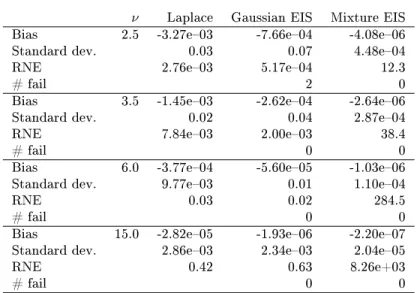
Results for this mixture EIS estimator are reported in the last column of Table 1 for values ofνranging from 2.5 to 15. The results reported are
the mean bias, the standard deviation and Geweke (1989) relative numer-ical eciency (RNE) factor based upon 10000 independent replications of the complete algorithm using a simulation sample size ofM = 32 and 7
EIS iterations. The RNE of an IS density obtains as the ratio between the variance of the direct MC estimates obtained by using the natural sam-plerp(z)and the IS MC estimates. High RNE values are preferable. For
comparison, we also considered the IS estimators based upon a univari-ate Gaussian sampler forz resulting from a local Laplace approximation
of the target integrandg(z)p(z), as well as from a global Gaussian EIS
approximation as described in Section 2. The Laplace-IS and Gaussian-EIS algorithm are implemented using the same sample sizeM as for the
mixture EIS.
The results of the experiment indicate that the mixture EIS sampler clearly outperforms the Gaussian EIS and the Laplace sampler with re-spect to numerical accuracy: For all degrees of freedomν, the former has
a substantially smaller standard deviation and a signicantly higher RNE factor than the latter. In fact, the RNE for the mixture EIS exceeds in all cases 1, which is the benchmark value for the natural samplerp(z),
while the RNE for the univariate Gaussian samplers is smaller than 1. This indicates that the joint bivariate EIS sampler m(z, w; ˆa) provides
a better approximation to the augmented integral g(z)p(z|w)p(w) than
the univariate Gaussian EIS and Laplace samplers to the marginalized integralg(z)p(z). This is conrmed by Figure 1 which shows the target
integrandg(z)p(z)forν= 2.5(normalized such that it integrates to one)
together with the Gaussian EIS and Laplace sampling densities as well as the marginal density forzobtained from the joint EIS samplerm(z, w; ˆa).
Figure 1 also reveals that for low degrees of freedom ν, the Gaussian
Laplace sampler is subject to a thin-tail problem since its tails decay more quickly than those of the target integrand. Forν={2.5,3.5,6}this
translates into signicantly downward biased MC estimates with a bias ranging from 3.9 to 10.9 standard deviations (see Table 1).
3.2 Finite mixture EIS
Here we consider the case where the natural samplerp(z)of the integral
given by Equations (1) and (2) is a nite mixture of the form
p(z) =
l
X
i=1
p(z|wi)pi, (27)
where pi denotes the mixing proportion for the ith mixture component
withPl
i=1pi= 1, andp(z|wi) is a conditional density depending on the
parameterwi. We assume that all mixture componentsp(z|wi)belong to
the same exponential family of distribution, which is essential for simpli-cations of the calculations.
The integral (1) to be approximated has the augmented form
I=
Z l X
i=1
g(z)p(z|wi)pidz. (28)
EIS may then be implemented using a joint mixed EIS samplerm(z, i;a) =
m(z|wi, az)·miwith m(z|wi, az) = k(z, i;az) χz(i, az) , χz(i, az) = Z k(z, i;az)dz, (29)
and EIS mixing proportions
mi= ki ¯ χ, χ¯= l X i=1 ki, i= 1, ..., l, (30)
wherea= (az, k1, ..., kl). This allows us to rewrite the integral (28) as I= ¯χ Z l X i=1 g(z)p(z|wi) k(z, i;az) χz(i, az)pi ki m(z, i;a)dz. (31)
The density kernelk(z, i;az)used to approximateg(z)p(z|wi)can be
specied as a parametric extension ofp(z|wi)as
k(z, i;az) =p(z|wi)ζ(z, az), (32)
where ζ is a kernel for a density belonging to the same parametric class
as p(z|wi). Sincep(z|wi) is assumed to be a member of the exponential
family,k(z, i;az)itself denes a kernel for a density of the same parametric
class asp(z|wi). From the factor in the rightmost bracket of (31), we see
that by setting the non-normalized mixing proportions of the importance density to
ˆ
ki(`+1)=χz(i,ˆaz(`+1))·pi i= 1, ..., l, (33)
we obtain a further simplied expression for (28):
I= ¯χ Z g(z) ζ(z, az) l X i=1 m(z, i;a)dz. (34)
Under this specication ofk(z, i;az)andki, i= 1, . . . , l, the EIS auxiliary
parametersaare obtained from the solution of the LS regression
min az,cz M X j=1 h lng(z(j,`))−cz−lnζ(z(j,`), az) i2 . (35)
Here{z(j,`), j= 1, ..., M}are draws from the step-`intermediate marginal
sampling densitym(z; ˆa(`))associated with the joint density m(z, i; ˆa(`)) =m(z|wi,ˆa
(`)
z )·mˆ
(`)
i . In order to simulate from the marginal EIS density
m(z; ˆa(`))using CRNs, we can rely upon the cdf inversion technique2.
2Whenm(z, wi;a)is Gaussian, as it is the case in the examples below, we use the approxi-mation erfcc given in Press et al. (2007) to the complementary error function involved in the relevant Gaussian cumulative distribution functions.
Since the marginal EIS densitym(z; ˆa)is analytically available, we can
directly use it to obtain the MC-EIS estimate of the integralI as
ˆ I= 1 M M X j=1 g(z(j))p(z(j)) m(z(j); ˆa) , (36)
and do not need to rely upon the joint EIS sampler for the augmented integral.
In order to illustrate this nite mixture EIS approach, consider the MC estimation ofR
g(z)p(z)dz, where g(z) is aN(0,exp{z})density for
yevaluated aty= 3, andp(z)is a zero mean and unit variance Gaussian
mixture of the form p(z)∼N(0, σ21)p1+N(0, σ22)p2 with p1 =p2 = 0.5
andσ2
2= 2−σ21. In this case, the augmented integrand (28) consists of
g(z) ∝ expn−1 2(3 2 e−z+z)o (37) p(z|wi) ∝ (σi2) −1/2 expn−1 2( z σi )2o, i= 1,2. (38)
The joint mixed density kernel meant to approximateg(z)p(z|wi)is
spec-ied as k(z, i;az) =p(z|wi)ζz(z;az), where (39) ζz(z;az) = exp n −1 2(αz 2 −2βz) o ,
with az = (α, β). The corresponding EIS density for z|wi is given by
m(z|wi, az)∼N(βσi2/[1 +ασ2i], σi2/[1 +ασi2]), and the EIS values of the
auxiliary parameters (α, β) are obtained from solving the LS problem
(35) where{lng(z(j,`))} is regressed on {[z(j,`)]2, z(j,`)}and a constant.
The expression for the integrating factor of k(z, i;az), which is used to
construct the EIS mixing proportionsmi dened in Equations (30) and
(33), is χz(i, az) = (1 +ασi2) −1/2 expn1 2 σi2β 2 1 +ασ2 i o . (40)
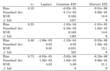
Table 2 summarizes the results for the nite mixture EIS estimates of the integral for values of σ1 ranging from 0.1 to 0.75. Note that for σ1 ≤0.25the target integrand is bimodal and forσ1 ≤0.4it is not
log-concave. As in the example in section 3.1, we also computed the MC estimates of the integral using the Gaussian EIS sampler and, in cases where the integrand is uni-modal, the Laplace sampler. The results in Table 2 are the mean biases, standard deviations and RNEs from 10,000 replications of the full procedure each based upon a simulation sample size of M = 32 and 7 EIS iterations. The results of the experiment
reveal that in all cases the mixture EIS sampler performs well leading to numerically very accurate estimates. As expected, the Gaussian samplers perform poorly when the integrand is bimodal and/or not log-concave. In those cases, the EIS iterations for the Gaussian EIS sampler often failed to converge indicating a severe mismatch between the target integrand and the class of Gaussian densities. In sharp contrast, we have found that the EIS convergence for the mixture EIS is fast indicating the adequacy of the class of Gaussian mixture samplers. This is conrmed by Figure 2 which shows the target integrand forσ1= 0.1together with the mixture
EIS density and the Gaussian EIS density.
4 High-dimensional mixture EIS
In this section we discuss operational implementations of the mixture EIS approach for high-dimensional integration required for a likelihood analy-sis of realistic models. Those high-dimensional implementations combine data augmentation steps as discussed for univariate problems in the previ-ous section with the generic sequential EIS approach for high-dimensional problems introduced in Section 2.1.
4.1 Example: student-
t
state-space model
We start to analyze a state space model with student-tmeasurement
er-rors, which represents a useful extension of the linear Gaussian specica-tion used, e.g. by Barndor-Nielsen and Shephard (2002) and Bach and Christensen (2011) to model time series of realized volatilities of asset returns.
The log of the daily realized volatility denoted by yt is assumed to
follow the process
yt = λt+σyut (41)
λt = µ+φ(λt−1−µ) +σλt, (42)
where(ut, t)are mutually independent iid variables with zero mean and
unit variance. For the measurement error ut we assume a standardized
student-tdistribution withν >2degrees of freedom, while the shock in
the latent state equationt is normally distributed.
The conditional distribution ofyt|λtdenes a student-tdensity kernel
for λt. In light of the rst pilot example, the use of (E)IS procedures
for the likelihood evaluation based on Gaussian sampling densities for the λts appears to be inadequate. However, the interpretation of the
fat-tailed student-tdistribution as a scale mixture of Normals allows us
to augment the state space model (41) and (42) in such a way that we can evaluate the likelihood via the sequential EIS outlined in Section 2.1 using convenient sampling densities from the exponential class. The rst step of data augmentation consists in representing the student-terror as ut ∼N(0,1/ηt−1), where ηt−1 ∼Gamma(ν/2,2/(ν−2)). In the second
step, we use the inverse cdf of the Gamma(ν/2,2/(ν−2))-distribution,
a standard normal variable
ηt=FΓ−1[Φ(wt)]≡hν(wt), wt∼N(0,1). (43)
This augmentation scheme allows us to recast the non-Gaussian linear state space model (41) and (42) into a non-linear one with a Gaussian measurement density given by
g(yt|λt, wt−1)∝hν(wt−1)1/2exp n −hν(wt−1) 2σ2 y (yt−λt)2 o , (44)
and two Gaussian state-transition densities
p(λt|λt−1) ∝ exp n − 1 2σ2 λ [λt−µ(λt−1)]2 o (45) p(wt−1) ∝ exp{− 1 2w 2 t−1}, (46)
whereµ(λt−1) =µ+φ(λt−1−µ). As we shall see below, the time shift of
the auxiliary variablewt relative toutandyttogether with the
represen-tation ofηtas a function of the Gaussian variablewtallows us to factorize
the integrand of the likelihood integral period-by-period into simple bi-variate Gaussian density kernels for the latent state variables(λt, wt).
Letzt0 = (λt, wt),zT =λT, andz0(t) = (z 0 0, ..., z
0
t)and assume for the
initial condition λ0 the stationary distribution λ0 ∼ N(µ, σ2λ/(1−φ
2
)).
Then the likelihood for the augmented state space representation (44)-(46) is given by L(ψ) = Z T Y t=0 ϕt(z(t))dz(T), (47) with ϕt(z(t)) = g(yT|λT, wT−1)p(λT|λT−1), t=T g(yt|λt, wt−1)p(λt|λt−1)p(wt), t= 1, ..., T−1 p(λ0)p(w0), t= 0, (48)
andψ= (µ, σy, ν, φ, σz)0.
In order to apply the sequential EIS of Section (2.1) to this augmented likelihood, we rst note that the factor g(yt|λt, wt−1)p(λt|λt−1) of the
period-tintegrand (48) denes a kernel of aN(m∗t, vt∗)distribution forλt
with m∗t = σy2µ(λt−1) +hν(wt−1)σ2λyt hν(wt−1)σλ2+σy2 , vt∗= σy2σ2λ hν(wt−1)σλ2+σy2 , (49)
and thatp(λ0)and p(wt)present Gaussian densities. It follows that for
t < T the period-t integrands ϕt dene bivariate Gaussian kernels in
zt, while the period-T integrand ϕT is a univariate Gaussian kernel for
zT =λT.
This immediately suggests to specify the EIS density kernels kt of
the period-t importance samplers mt in Equation (10) as the following
parametric extensions of the Gaussian kernelsϕt:
kt(z(t), at) =ϕt(z(t))ζt(zt, at), (50) with ζt(zt, at) = exp n −1 2(z 0 tPtzt−2R0tzt) o , t= 0, ..., T−1, (51)
andζT(·)≡1. HerePtis a symmetric(2×2)matrix andRta(2×1)vector
representing the EIS auxiliary parameters, i.e. at= (vech(Pt)0, Rt0)0. Since
ϕt and ζt represent Gaussian density kernel for zt, it follows the EIS
samplersmt associated withkt are Gaussian distributions forzt|z(t−1).
Using this parametrization ofkt and rewriting the likelihood integral
(47) according to Equation (12) leads to
L(ψ) =χ0(a0) Z T−1 Y t=0 χt+1(z(t), at+1) ζt(zt, at) T−1 Y t=0 mt(zt|z(t−1), at)dz(T−1). (52)
zT =λT can be done analytically and amounts to computing the integral
R
mT(zT|zT−1, aT)dzT, which is equal to 1. It immediately follows that
the EIS auxiliary regressions in Equation (13) simplify into a sequence of T linear LS regressions of {lnχt+1(z (j,`) (t) ,aˆ (`+1) t+1 )} on a constant and {[λ(tj,`)]2,[w(j,`) t ] 2,[λ(j,`) t ·w (j,`) t ], λ (j,`) t , w (j,`) t }fort=T−1, ...,0. As initial samplers{mt(zt|z(t−1),ˆa (0)
t )}we use the Gaussian distributions associated
with the Normal density kernels given in Equation (48). Details of the implementation of this sequential mixture EIS application are provided in Appendix A.
The data we use to estimate the student-t state space model (41)
and (42) by ML based upon sequential mixture EIS consists of the daily realized variances computed for the returns of the IBM stock traded at the New York Stock Exchange. We useT = 2156daily observations from
January 1, 2000 until July 30, 2008. The daily realized variances can be computed asrvt =PJτ=1x2t,τ wherext,τ is the return computed for the
τs 5-minute interval of trading dayt(This data set is discussed in more
details in Chiriac and Voev (2011)).
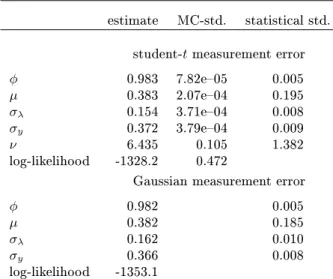
The ML EIS results based upon a simulation sample sizeM = 64and
4 EIS iterations are summarized in Table 3. The parameter estimates and their MC (numerical) standard deviations are computed as the means and standard deviations of 100 ML estimates conducted under dierent sets of CRNs. The statistical standard deviations are obtained from 500 ML estimates for articial data generated from the model. Total computing time for a full ML optimization using a BFGS optimizer is of the order of 1 min on a Dell PowerEdgeR200 computed with 2.66 GHz Quad core processor for a code written in Fortran 90. For comparison, we also report the ML estimation results for the state space model (41) and (42) with Gaussian measurement errorsutobtained as the limit forν→ ∞, in which
case we can use the standard Kalman lter to evaluate the likelihood. The MC standard deviations indicate that the ML estimates based on
the mixture EIS approach are numerically very accurate. The estimated degrees of freedomν is 6.4, indicating a large deviation from normality.
The substitution of the Normal for the student-tdistribution decreases the
value of the maximized likelihood function by 25, indicative of a signicant deterioration in t. Finally note that the strong persistence with a value ofφclose to one is typical for volatility models for asset returns.
4.2 Example: stochastic volatility model with
jumps
In order to illustrate the mixture EIS approach for high-dimensional in-tegration when the target integrand involves nite mixtures, we consider the ML estimation of a discrete-time stochastic volatility (SV) model with leverage eects and jumps (see, e.g., Yu (2005); Durham (2006) for a dis-cussion of the discrete-time SV model and Eraker et al. (2003); Malik and Pitt (2011) for SV models involving jumps).
The stock log-returnsytare assumed to follow the process
yt=γ+σyexp{zt−1/2}(ρηt+
p
1−ρ2ξ
t) +Jtσuut (53)
and the latent volatility factor
zt=φzt−1+σzηt. (54)
HereJtrepresents the time-tjump arrival, which follows a Bernoulli
pro-cess with state probabilitiesP(Jt =j) =pj with j∈ {0,1}. The jump
size is given by σuut, where ut ∼ N(0,1). The innovations ηt and ξt
are assumed to be independent fromut and are normally distributed as
(ηt, ξt)∼N(0, I), whereI is the identity matrix. The parameterρ
mea-sures the leverage eect, whileσuandp1represent the average jump size
and jump intensity respectively.
conditional density ofzt andyt givenzt−1 andJt is a bivariate Gaussian
density, which can be factorized as
p(zt, yt|zt−1, Jt) =p(zt|yt, zt−1, Jt)p(yt|zt−1, Jt), (55)
wherep(zt|yt, zt−1, Jt) andp(yt|zt−1, Jt) are conditional Gaussian
densi-ties forzt andyt given by
p(zt|yt, zt−1, Jt) ∼ N(µzt, σ 2 zt) (56) p(yt|zt−1, Jt) ∼ N(γ, σy2t), (57) with µzt = φzt−1+ (yt−γ) ρσyσzexp{zt−1/2} σ2 yexp{zt−1}+Jtσu2 (58) σ2zt = σ 2 z(1− σy2exp{zt−1} σ2 yexp{zt−1}+Jtσ2u ) (59) σy2t = σ 2 yexp{zt−1}+Jtσu2. (60)
Based on this factorization ofp(zt, yt|zt−1, Jt), the likelihood function
obtains asL(ψ) =R QT t=0ϕt(z(t))dz(T), where ϕt(z(t)) = P j∈{0,1}p(zt|yt, zt−1, Jt)p(yt|zt−1, Jt)pj, t= 1, ..., T p(z0), t= 0, (61) and ψ = (γ, σy, σu, σz, ρ, φ, p1)0. The initial conditionz0 is assumed be
generated by the stationary distribution asz0∼N(0, σ2z/(1−φ2)).
In order to apply sequential EIS outlined in Section 2.1 to the evalua-tion of this likelihood funcevalua-tion, we rst note that fort≥1the factorϕtin
the likelihood integral denes a density kernel for a two-component normal mixture distribution forzt|zt−1 with non-normalized mixing proportions p(yt|zt−1, Jt)pj. The corresponding proper density for this two-component
normal mixture distribution obtains as p∗(zt|zt−1) = ϕt(z(t)) p(yt|zt−1) = X j∈{0,1} p(zt|yt, zt−1, Jt)πJt, (62)
where the normalized mixing proportionsπJt are
πJt= p(yt|zt−1, Jt)pj p(yt|zt−1) with p(yt|zt−1) = X j∈{0,1} p(yt|zt−1, Jt)pj. (63)
Using the normalized factors of the likelihood integral in Equation (62) we can rewrite the likelihood as
L(ψ) =
Z T−1 Y
t=0
p(yt+1|zt)p∗(zt|zt−1)dz(T−1), (64)
with p∗(z0|z−1) = p(z0). The integration w.r.t. the variable zT is done
analytically and amounts to computingR
p∗(zT|zT−1)dzT which is equal
to 1.
Clearly, (E)IS approaches based on (E)IS densities for the zts from
the exponential family are not adequate to approximate this likelihood function involving nite mixtures leading to a possibly bimodal target integrand. Instead we shall specify the EIS density kernelkt in Equation
(11) as the following parametric extension of the natural Gaussian mixture samplerp∗given in Equation (62):
kt(z(t), at) = p ∗ (zt|zt−1)ζt(zt, at) (65) = P j∈{0,1}p(zt|yt, zt−1, Jt)ζt(zt, at)πJt, t≥1 p(z0)ζ0(z0, a0), t= 0, where ζt(zt, at) = exp n −1 2(αtz 2 t −2βtzt) o , t= 0, ..., T−1, (66)
for period t = 0 the EIS sampler m0(z0;a0) = k0(z0, a0)/χ0(a0) is a
simple Gaussian density, while for t ≥ 1 the corresponding EIS
den-sities mt(zt|z(t−1), at) are two-component Gaussian mixtures associated
with the joint mixed density kernelp(zt|yt, zt−1, Jt)ζt(zt, at)πJt forztand
Jt. The corresponding EIS densities forzt obtain as mt(zt|z(t−1);at) =
P
j∈{0,1}mt(zt|z(t−1), Jt;at)mJt, where the Gaussian EIS mixture
com-ponentsm(zt|z(t−1), Jt;at)are mt(zt|z(t−1), Jt;at) = p(zt|yt, zt−1, Jt)ζt(zt, at) χt(z(t−1), Jt, at) , (67) χt(z(t−1), Jt, at) = Z p(zt|yt, zt−1, Jt)ζt(zt, at)dzt, (68)
and the resulting EIS mixing proportionsmJt obtain as
mJt = χt(z(t−1), Jt, at)πJt χt(z(t−1)at) , (69) χt(z(t−1), at) = X j∈{0,1} χt(z(t−1), Jt, at)πJt. (70)
It immediately follows thatχt(z(t−1), at)as given in Equation (70)
repre-sents the integrating factor for the EIS density kernelkt(z(t), at)in
Equa-tion (65) such that the EIS density can be represented asmt(zt|z(t−1);at)
=kt(z(t), at)/ χt(z(t−1), at).
Finally note that using the parametrization of the density kernelktfor
the EIS density given in Equations (65) and (66), the likelihood function (64) can be rewritten according to Equation (12) as
L(ψ) =χ0(a0) Z "T−1 Y t=0 χt+1(z(t), at+1)p(yt+1|zt) ζt(zt, at) # (71) × T−1 Y t=0 mt(zt|z(t−1), at)dz(T−1),
withχT ≡1. Hence, the EIS auxiliary regressions in Equation (7)
sim-plify into a sequence ofT linear LS problems where{ln[χt+1(z (j,`)
t ,ˆa
(`+1)
p(yt+1|zt(j,`))]} is regressed on a constant and {[z (j,`) t ] 2 , zt(j,`)} for t = T −1, ...,0. As initial samplers{mt(zt|z(t−1),aˆ (0)
t )}we let logζt match
the two rst derivatives of logp(yt+1|zt, Jt+1 = 0) around the mode for t= 0, . . . , T−1. This amounts to setting αt = 1 andβt = log{[(yt+1− γ)/σy]2}. Details of the implementation of this sequential nite mixture
EIS application are provided in Appendix B. Before presenting the em-pirical results, an important remark is in order. As described above, the EIS implementation requires to approximateχt+1(z(t), at+1)p(yt+1|zt)by
a Gaussian kernelζt(zt, at), where bothχt+1(z(t), at+1)andp(yt+1|zt)are
weighted sums of two functions inzt (see Equations 63 and 70). Hence,
theoretically there is no guarantee that their product will dene a well-behaved function inzt. However, we have found that those products are
very accurately approximated by the Gaussian kernelsζt(zt, at). In fact,
theR2s of the EIS auxiliary regressions are typically larger than 0.99.
The data we use to estimate the SV model (53) and (54) by ML based upon sequential nite mixture EIS consists of daily continuously com-pounded log-returns on the S&P500 stock price index from January 3, 2000 to December 31, 2007 with T = 2008. The ML-EIS results based
upon a simulation sample size M = 32 and 10 EIS iterations are
sum-marized in Table 4. The parameter estimates and their MC standard deviations are computed as the means and standard deviations of 100 ML estimates obtained under dierent sets of CRNs. The statistical standard deviations are based upon 500 ML estimates for articial data from the model. Total computing time for a full ML estimation using a BFGS op-timizer is 142 seconds for a Fortran 90 code on a laptop computer with an Intel core i7 processor with 8 Gb of memory using 2 cores in parallel. For comparison, we also estimate the corresponding SV model without jumps (obtained by letting eitherσu→0orp1→0) using the same code
and same simulation sample size as above. In this case, the mixture-EIS procedure boils down to a standard EIS algorithm based on Gaussian IS
densities. The MC standard deviations reported in Table 4 reveal that the ML parameter estimates for the SV model with jumps based on nite mixture EIS are numerically very accurate. In fact, the MC standard deviations for the SV jump model are of the same order of magnitudes as those obtained by the standard EIS procedure for the ML estimation of the model without jumps. The value of the likelihood ratio statistic for the hypothesisH0 : σu= 0, p1 = 0is 10.2, indicating a rejection of the
model without jumps against the SV jump specication at the 1% level. The estimate of the jump intensity parameterp1implies that jumps occur
at a fairly low frequency with an average of 173 trading days between two jumps. This result is consistent with the ndings of Eraker et al. (2003) and Malik and Pitt (2011). The high persistence with a value ofφclose
to 1 and the strong leverage eect with a signicantly negative value ofρ
is typical of SV models.
5 Discussion
In this paper, we propose ecient importance sampling (EIS) procedures for the evaluation of likelihood functions involving nite or innite mix-tures leading to possibly ill-behaved target densities with multiple modes or fat tails. Our approach exploits the mixture specication of the target density and uses a data augmentation step, demarginalizing the mixture density to include the mixing variable as an additional latent variable.
In the examples used to illustrate our mixture EIS approach, we have found that this extension of the space of integration can lead to well behaved target integrands for the extended space which can be well glob-ally approximated by standard distributions belonging to the exponential family.
The set of examples considered here do by no means deplete the po-tential area of application of the mixture EIS. Further examples where we
have also successfully applied this methodology include the model of Cox et al. (1985) observed with Gaussian measurement noise (exploiting that the transition law of the CIR-diusion is a Poisson-mixture of Gammas) and a time-discretized jump-diusion model observed with measurement noise.
As for most other (E)IS methods, mixture EIS involves a high degree of tailor-making for each particular model. However, many latent vari-able models today involve implicitly or explicitly some form of mixing or hierarchical structures, generating non-Gaussian and dependent target densities. In so far, the demarginalization step underlying the mixture EIS can in many cases be quite automatic.
As shown in the two high-dimensional examples, complex latent vari-able models are generally needed to capture the salient features of eco-nomic data. However, such complex models often give rise to integration problems involving high-dimensional and complex target densities. Thus may the required exibility come at the cost of making the models dicult to t to the data. We think that the mixture EIS provides a useful and ef-cient procedure for likelihood-based inference for such non-standard, but generally more appropriate models. The estimation can be done without imposing severe restrictions on the model building, while retaining the sparsely parameterized local importance densities and computationally simple LS regressions of the exponential family EIS.
Appendix A
This appendix details the implementation of the sequential mixture EIS application for the MC likelihood evaluation of the student-tstate space
model (41) and (42) outlined in Section 4.1.
The sequence of EIS density kernels kt (t = 0, ..., T) as dened by
Equations (48), (50), and (51) and the corresponding integrating factors
χthave the following functional forms:
For t =T the univariate Gaussian kernel kT =ϕT forZT = λT is
given by kT(z(T)) = ϕ∗T(zT−1) 2πσyσλ expn−1 2 λ2 T v∗ T −2m ∗ T v∗ T λT o , (72) where ϕ∗T(zT−1) =hν(wT−1)1/2exp n −1 2 hν(wT−1)y2 T σ2 y +µ(λT−1) σ2 λ o , (73)
andm∗T andv∗T are dened by Equation (49). Integrating the Gaussian
kernelkT w.r.t.λT and omitting irrelevant constants leads to
χT(z(T−1))∝ϕ ∗ T(zT−1)vT∗1/2exp n1 2 mT∗2 v∗ T o . (74)
Fort= 1, ..., T−1the bivariate Gaussian kernelkt=ϕt·ζtforzthas
the form kt(z(t), at) = ϕ∗t(zt−1) (2π)3/2σ yσλ expn−1 2 zt0(Σ −1 t +Pt)zt (75) −2(µ0tΣ −1 t +R 0 t)zt o , where ϕ∗t(zt−1) =hν(wt−1)1/2exp n −1 2 hν(wt−1)y2 t σ2 y +µ(λt−1) σ2 λ (76)
−mt ∗2 v∗ t +µ0tΣ −1 t µt o
and the mean and variance associated with the density kernelϕtare given
as µt= (m∗t,0) 0 , Σt= vt∗ 0 0 1 . (77)
It follows that the EIS samplermtforzt|z(t−1)associated with the density
kernel (75) is a bivariate Gaussian distribution with mean and variance given by µ∗t = Σ ∗ t(Σ −1 t µt+Rt), Σ ∗ t = (Σ −1 t +Pt) −1 , (78)
Integrating the Gaussian kernelktw.r.t.zt leads to
χt(z(t−1), at)∝ϕ ∗ t(zt−1)|Σ ∗ t|1/2exp n1 2µt ∗0 Σt ∗−1 µ∗t o . (79)
Fort= 0the bivariate Gaussian kernelk0=ϕ0·ζ0 forz0 has the form
k0(z0, a0) =ϕ ∗ 0exp n −1 2 z00(Σ −1 0 +P0)z0−2(µ 0 0Σ −1 0 +R 0 0)z0 o , (80) where ϕ∗0= (1−φ2)1/2 2πσλ expn−1 2µ 0 0Σ −1 0 µ0 o , (81) µ0= (µ,0) 0 , Σ0= σ2 λ/(1−φ2) 0 0 1 . (82)
It follows that the EIS sampler m0 for z0 associated with the density
kernel (80) is a bivariate Gaussian distribution with mean and variance given by µ∗0= Σ ∗ 0(Σ −1 0 µ0+R0), Σ∗0= (Σ −1 0 +P0)−1. (83)
Integrating the Gaussian kernelk0w.r.t.z0 leads to
χ0(a0) = 2πϕ∗0|Σ ∗ 0| 1/2 expn1 2µ0 ∗0 Σ0∗−1µ∗0 o . (84)
Appendix B
In this appendix we provide details for the implementation of the sequen-tial nite mixture EIS application for the MC likelihood evaluation of the SV model with jumps (53) and (54) outlined in Section 4.2.
The sequence of EIS densitiesmt(zt|z(t−1), at)associated with the
den-sity kernelskt(z(t), at)dened in Equations (65) and (66) and the
corre-sponding integrating factors χt(z(t−1), at) such that mt(zt|z(t−1);at) =
kt(z(t), at)/ χt(z(t−1), at)obtain as follows:
Fort= 1, ..., T−1the EIS density is a two-component mixture,
mt(zt|z(t−1);at) =
X
j∈{0,1}
mt(zt|z(t−1), Jt;at)mJt, (85)
where the mixture component mt(zt|z(t−1), Jt;at) and the mixing
pro-portionsmJt are dened by Equations (67) and (69), respectively. The
density kernel for the mixture componentmt(zt|z(t−1), Jt;at)has the form
(see Equation 67) p(zt|yt, zt−1, Jt)ζt(zt, at) = 1 √ 2πσzt exp n −1 2 h 1 σ2 zt +αt i zt2 (86) −2hµzt σ2 zt +βt i zt+ µ2zt σ2 zt o , whereµzt andσ 2
zt are dened in Equations (58) and (59). It follows that
the EIS mixture componentmt(zt|z(t−1), Jt;at)is a Gaussian density with
mean and variance given by
µ∗t =σ ∗ t 2µzt σ2 zt +βt , σt∗ 2 = σ 2 zt 1 +αtσz2t . (87)
Integrating the Gaussian kernel (86) w.r.t.zt leads to the following form
of the integrating factor given by Equation (68):
χt(z(t−1), Jt, at) = σt∗ σzt expn1 2 µ2z t σ2 zt −µ ∗ t 2 σ∗ t2 o . (88)
Based upon this integrating factor for the mixture component, we can compute the mixing proportionsmJtand the integrating factorχt(z(t−1), at)
associated with the EIS density kernel according to Equations (69) and (70).
Fort= 0the EIS density kernelkt(z0;a0) dened in Equations (65)
and (66) has the form
p(z0)ζ0(z0, a0) = (1−φ2)1/2 √ 2πσz expn−1 2 h1−φ2 σ2 z +α0 i z20−2β0z0 o . (89)
It follows that the EIS samplerm0forz0 is a Gaussian distribution with
mean and variance given by
µ∗0=σ ∗ 0 2 β0, σ ∗ 0 2 = σ 2 z/(1−φ2) 1 +α0σz2/(1−φ2) . (90)
Integrating the Gaussian kernel (89) w.r.t.z0 leads to the following form
of the integrating factor
χ0(a0) = (1−φ2)1/2σ∗0 σz exp n −1 2 µ∗ 02 σ∗ 0 2 o . (91)
For the this model, we slow down the convergence of the EIS iterations by choosing shorter step-lengths. This is done in order to reduce the probability of getting ana(`)corresponding to zero variance or some other
pathology in the rst iterations. In practice, this done by settinga(t`+1)←
sa(t`+1)+ (1−s)a
(`)
t withs= min(1,exp(−0.6 + 0.1`))immediately after
References
Ardia, D., L. F. Hoogerheide, and H. K. van Dijk (2009, 1). Adaptive mixture of student-t distributions as a exible candidate distribution for ecient simulation: The r package admit. Journal of Statistical Software 29 (3), 132.
Bach, C. and B. J. Christensen (2011). Latent integrated stochastic volatility, realized volatility, and implied volatility: A state space ap-proach. CREATES Research Papers 2010-61, School of Economics and Management, University of Aarhus.
Barndor-Nielsen, O. E. and N. Shephard (2002). Econometric analy-sis of realized volatility and its use in estimating stochastic volatility models. Journal of the Royal Statistical Society. Series B (Statistical Methodology) 64 (2), pp. 253280.
Bauwens, L. and F. Galli (2009). Ecient importance sampling for ML estimation of SCD models. Computational Statistics and Data Analy-sis 53, 19741992.
Chiriac, R. and V. Voev (2011). Modelling and forecasting multivariate realized volatility. Journal of Applied Econometrics, Forthcoming. Cox, J. C., J. E. Ingersoll, and S. A. Ross (1985). A theory of the term
structure of interest rates. Econometrica 53 (2), 385407.
Durbin, J. and S. J. Koopman (1997). Monte Carlo maximum likelihood estimation for non-Gaussian state space models. Biometrika 84 (3), 669684.
Durbin, J. and S. J. Koopman (2000). Time series analysis of non-gaussian observations based on state space models from both classi-cal and bayesian perspectives. Journal of the Royal Statisticlassi-cal Society Series B 62, 356.
Durham, G. B. (2006). Monte carlo methods for estimating, smoothing, and ltering one and two-factor stochastic volatility models. Journal of Econometrics 133, 273305.
Eraker, B., M. Johannes, and N. Polson (2003). The impact of jumps in volatility and returns. The Journal of Finance 58 (3), 12691300. Frühwirth-Schnatter, S. and H. Wagner (2006). Auxiliary mixture
sam-pling for parameter-driven models of time series of counts with appli-cations to state space modelling. Biometrika 93 (4), 827841.
Geweke, J. (1989). Bayesian inference in econometric models using monte carlo integration. Econometrica 57 (6), pp. 13171339.
Geweke, J. (1993). Bayesian treatment of the independent student- t linear model. Journal of Applied Econometrics 8 (S), S19S40. Hesterberg, T. (1995). Weighted average importance sampling and
defen-sive mixture distributions. Technometrics 37 (2), pp. 185194.
Jung, R. C., R. Liesenfeld, and J.-F. Richard (2011). Dynamic factor models for multivariate count data: An application to stock-market trading activity. Journal of Business and Economic Statistics 29 (1), 7385.
Kleppe, T. S., J. Yu, and H. J. Skaug (2010). Simulated maximum like-lihood estimation of continuous time stochastic volatility models. In W. Greene and R. C. Hill (Eds.), Maximum Simulated Likelihood Meth-ods and Applications (Advances in Econometrics, Volume 26), pp. 137 161. Emerald Group Publishing Limited.
Kloek, T. and H. K. v. Dijk (1978). Bayesian estimates of equation system parameters: An application of integration by monte carlo. Economet-rica 46, pp. 119.
Liesenfeld, R. and J.-F. Richard (2001). Monte carlo methods and bayesian computation: importance sampling. In N. Smelser and P. Baltes (Eds.), International Encyclopedia of the Social & Behavioral Sciences. Elsevier Science, Oxford.
Liesenfeld, R. and J.-F. Richard (2003). Univariate and multivariate stochastic volatility models: estimation and diagnostics. Journal of Empirical Finance 10, 505531.
Liesenfeld, R. and J.-F. Richard (2010). Ecient estimation of probit models with correlated errors. Journal of Econometrics 156 (2), 367 376.
Malik, S. and M. K. Pitt (2011). Modelling stochastic volatility with leverage and jumps: A simulated maximum likelihood approach via particle ltering. Documents de Travail 318, Banque de France. Press, W. H., S. A. Teukolsky, W. T. Vetterling, and B. P. Flannery
(2007). Numerical Recipes 3rd Edition: The Art of Scientic Comput-ing. Cambridge University Press.
Richard, J.-F. and W. Zhang (2007). Ecient high-dimensional impor-tance sampling. Journal of Econometrics 127 (2), 13851411.
Robert, C. P. and G. Casella (2004). Monte Carlo statistical methods. Springer.
Sandmann, G. and S. Koopman (1998). Maximum likelihood estimation of stochastic volatility models. Journal of Econometrics 63, 289306. Shephard, N. and M. K. Pitt (1997). Likelihood analysis of non-gaussian
measurement time series. Biometrika 84, 653667.
Yu, J. (2005). On leverage in a stochastic volatility model. Journal of Econometrics 127, 165178.
Table 1. IS integration for a student-tdensity.
ν Laplace Gaussian EIS Mixture EIS
Bias 2.5 -3.27e03 -7.66e04 -4.08e06 Standard dev. 0.03 0.07 4.48e04 RNE 2.76e03 5.17e04 12.3
# fail 2 0
Bias 3.5 -1.45e03 -2.62e04 -2.64e06 Standard dev. 0.02 0.04 2.87e04 RNE 7.84e03 2.00e03 38.4
# fail 0 0
Bias 6.0 -3.77e04 -5.60e05 -1.03e06 Standard dev. 9.77e03 0.01 1.10e04
RNE 0.03 0.02 284.5
# fail 0 0
Bias 15.0 -2.82e05 -1.93e06 -2.20e07 Standard dev. 2.86e03 2.34e03 2.04e05 RNE 0.42 0.63 8.26e+03
# fail 0 0
Note: IS-MC estimation ofR
g(z)p(z)dzwherepis a standardized student-tdensity withν
degrees of freedom, andgis aN[z,42]-density. IS simulation sample size isM= 32and the
number of EIS iterations is 7. Mean biases relative to the true value, standard deviations and RNEs are based upon 10000 replications under dierent CRN seeds. # fail denotes the
number of replications where the EIS approximation failed to converge. The true values of the integrals were computed using high precision numerical integration.
Table 2. IS integration for a two-component Gaussian mixture density.
σ1 Laplace Gaussian EIS Mixture EIS
Bias 0.10 -6.02e05 -9.81e06 Standard dev. 6.71e03 8.99e04
RNE 0.338 18.8
# fail 1457 0
Bias 0.25 -1.85e04 -1.01e05 Standard dev. 6.58e03 1.02e03
RNE 0.348 14.6
# fail 1493 0
Bias 0.40 -1.06e03 -1.52e04 -9.93e06 Standard dev. 0.02 0.02 1.08e03
RNE 0.05 0.031 13.1
# fail 335 0
Bias 0.75 -8.03e05 -3.02e06 -6.53e06 Standard dev. 1.92e03 1.83e03 8.96e04
RNE 4.62 5.09 21.1
# fail 0 0
Note: IS-MC estimation ofR
g(z)p(z)dzwherepis a Gaussian mixture of the form N(0, σ2
1)p1+N(0, σ22)p2withp1=p2= 0.5andσ22= 2−σ12, andgis aN[0,exp(z)]-density.
IS simulation sample size isM= 32and the number of EIS iterations is 7. Mean biases
relative to the true value, standard deviations and RNEs are based upon 10000 replications under dierent CRN seeds. # fail denotes the number of replications where the EIS approximation failed to converge. The true values of the integrals were computed using high
Table 3. ML estimation results for state space models for realized volatility.
estimate MC-std. statistical std. student-tmeasurement error φ 0.983 7.82e05 0.005 µ 0.383 2.07e04 0.195 σλ 0.154 3.71e04 0.008 σy 0.372 3.79e04 0.009 ν 6.435 0.105 1.382 log-likelihood -1328.2 0.472
Gaussian measurement error
φ 0.982 0.005
µ 0.382 0.185
σλ 0.162 0.010
σy 0.366 0.008
log-likelihood -1353.1
Table 4. ML estimation results for the SV model with leverage eects and jumps for returns.
estimate MC-std. statistical std. SV model with jumps
γ -1.80e-04 4.65e-05 0.018 σy 0.910 2.68e-04 0.097 σz 0.147 1.46e-04 0.015 ρ -0.889 5.21e-04 0.039 φ 0.985 2.43e-05 0.003 σu 1.484 0.020 0.760 log(p1) -5.156 0.046 1.658 log-likelihood -2718.7 0.060 Akaike 5451.4
SV model without jumps
γ -0.003 1.78e-05 0.019 σy 0.920 7.80e-05 0.091 σz 0.148 1.83e-04 0.013 ρ -0.875 4.70e-04 0.052 φ 0.985 3.01e-05 0.003 log-likelihood -2723.8 0.075 Akaike 5457.6
−30 −2 −1 0 1 2 3 4 0.1 0.2 0.3 0.4 0.5 0.6 0.7 0.8 0.9 1 integrand Laplace IS Gaussian EIS Mixture EIS
Figure 1. Target integrandg(z)p(z)(normalized such that it integrates
to 1) wherepis a standardized student-tdensity withν= 2.5degrees of
freedom andgis aN[z,42]-density, Gaussian Laplace IS sampling
density, Gaussian EIS sampling density, and marginal density forz
−10 0 1 2 3 4 5 0.1 0.2 0.3 0.4 0.5 0.6 0.7 0.8 0.9 1 integrand Gaussian EIS Mixture EIS
Figure 2. Target integrandg(z)p(z)(normalized such that it integrates
to 1) wherep(z)∼0.5·N(0, σ21) + 0.5·N(0, σ22)withσ22= 2−σ12, σ1= 0.1andgis aN[0,exp(z)]-density, Gaussian EIS sampling density,


![Figure 2. Target integrand g(z)p(z) (normalized such that it integrates to 1) where p(z) ∼ 0.5 · N(0, σ 21 ) + 0.5 · N (0, σ 2 2 ) with σ 2 2 = 2 − σ 1 2 , σ 1 = 0.1 and g is a N[0, exp(z)]-density, Gaussian EIS sampling density,](https://thumb-us.123doks.com/thumbv2/123dok_us/1452326.2694405/44.918.272.663.188.507/figure-target-integrand-normalized-integrates-density-gaussian-sampling.webp)
