Efficient High-Dimensional Importance
Sampling
Jean-Francois Richard
University of Pittsburgh
and
Wei Zhang
National University of Singapore
March 31, 2005
Abstract
The paper describes a simple, generic and yet highly accurate Ef-ficient Importance Sampling (EIS) Monte Carlo (MC) procedure for the evaluation of high-dimensional numerical integrals. EIS is based upon a sequence of auxiliary weighted regressions which actually are linear under appropriate conditions. It can be used to evaluate like-lihood functions and byproducts thereof, such as ML estimators, for models which depend upon unobservable variables. A dynamic sto-chastic volatility model and a logit panel data model with unobserved heterogeneity (random effects) in both dimensions are used to provide illustrations of EIS high numerical accuracy, even under small number of MC draws. MC simulations are used to characterize the finite sam-ple numerical and statistical properties of EIS-based ML estimators.
Keywords: Monte Carlo, Importance Sampling, Marginalized Like-lihood, Stochastic Volatility, Random Effects.
1
Introduction
Monte Carlo (hereafter MC) simulation techniques provide a powerful tool to numerically evaluate expectations of functions of random variables for which no analytical expressions are available. See e.g., Fishman (1996) for an in-depth analysis of MC concepts and algorithms. One particular area where MC methods play a critical role is that of models which incorporate large numbers of unobserved random variables. Examples to be discussed further below are stochastic volatility models in finance and large panels with unobserved heterogeneity, where dimensions of integration can be in the thousands. It has long been recognized that the feasibility of evaluating such high-dimensional integrals by MC simulation critically depends on the selection of efficient MC samplers. Importance Sampling which consists of replacing an inefficient initial sampler by a more efficient auxiliary sampler is conceptually well suited for that purpose. Its weakness lies in the current lack of generic algorithms to construct Efficient Importance Samplers (hereafter EIS) at a sufficiently broad level of generality.
The object of the present paper is to propose a new algorithm to construct EIS, which is generic and particularly well adapted to (very) high-dimensional MC integration. In particular, under appropriate simplifying conditions it amounts to a simple recursive sequence of auxiliary least squares optimization problems which, as we shall illustrate below, can produce enormous efficiency gains at low cost of computation.
The paper is organized as follows: Section 2 introduces Importance Sam-pling. The generic principle of EIS is introduced in Section 3. Its high-dimensional implementation is presented in Section 4. Numerical and sta-tistical properties of EIS based estimates are analyzed in Section 5. Pilot applications of EIS to stochastic volatility and panel models are presented in Section 6; Section 7 concludes.
2
Importance Sampling
2.1
Principle
Importance Sampling (hereafter IS) has been around for quite some time. Early descriptions of the method can be found e.g. in Kahn and Marshall (1953), Trotter and Tukey (1956) or Hammersley and Handscomb (1964,
Section 5.4). See also Fishman (1996, Section 4.1) for a more recent in-depth presentation of IS. In this section we briefly introduce the concept of IS, establishing notation for our subsequent analysis.
Assume one has to evaluate a functional integral of the form
G(δ) =
Z
X
g(x, δ)·p(x|δ)·dx
(1)
where g denotes a function which is integrable in x with respect to (w.r.t.) a densityp(x|δ) with supportX. Let θ, y andλ denote parameters, observa-tions and latent variables, respectively. Applicaobserva-tions requiring the evaluation of integrals of the form given in (1) are: (i) The Bayesian evaluation of pos-terior moments for which δ=yandx= (θ, λ); (ii) The (classical) evaluation of marginalized likelihood functions for which δ = (θ, y) and x = λ; (iii) The computation of Generalized Method of Moment estimators for which
δ = θ and x = (y, λ). Examples of marginalized likelihood evaluations are presented in Section 6 below.
The factorization under the integral sign in equation (1) is typically as-sociated with the initial formulation of one’s statistical model and we shall accordingly refer to p as to an initial sampler. An initial MC estimate of
G(δ) is given by GS(δ) = 1 S S X i=1 g(˜xi, δ) (2)
where the ˜xi’s are independently identically distributed (i.i.d.) draws from
p. If, however, the sampling variance of g w.r.t. x is (very) large, accurate estimation of Gmay require prohibitively large numbers of draws. Dramatic illustrations of such inefficiency will be provided in Section 6 below.
Importance Sampling consists of replacing the initial sampler p(x|δ) by an auxiliary parametric importance sampler m(x|a), rewriting equation (1) as G(δ) = Z X g(x, δ)·w(x;δ, a)·m(x|a)dx (3) with w(x;δ, a) = p(x|δ) m(x|a) (4)
The corresponding IS-MC estimate of G(δ) is given by
GS;m(δ, a) = 1 S S X i=1 w(˜xi;δ, a)·g(˜xi;δ) (5)
where the ˜xi’s now denote i.i.d. draws from m(x|a). The MC sampling variance of Gs;m is given by V[GS;m(δ, a)] = 1 SG(δ)·V(a;δ) (6) with V(a;δ) = 1 G(δ) Z X ϕ(x;δ) m(x|a)−G(δ) 2 m(x|a)dx (7) ϕ(x;δ) =g(x, δ)·p(x|δ) (8)
Clearly, one’s objective in selectingm(x|a) - ora∈Aonce a class of samplers
M = {m(x|a);a ∈ A} has been preselected - should be that of minimizing
V(a;δ) w.r.t. a for any given δ. Conditions for the finiteness of V(a;δ) are discussed e.g. in Geweke (1996) or Stern (1997). Nevertheless, the critical convergence issue of whether a Central Limit theorem applies to√s(Gs;m−G)
remains difficult to verify in complicated and/or high-dimensional IS appli-cations and will be discussed further below.
Note that the term Importance Sampling emphasizes the fact thatm(x|a) is designed to sample mostly from the important part of S(δ) i.e.,. from those parts of S(δ) which contribute most to the value of the integral. Such terminology can be somewhat misleading since it is now well recognized that large or even infinite values of V(a;δ) typically originate from the far tails of m(x|a) which is precisely why IS pathologies can be empirically hard to detect.
Clearly, the two critical issues to be addressed in IS applications are (1) the selection of an appropriate class M of auxiliary samplers; and (2) the selection of an efficient sampler within M i.e. one for which V(a;δ) is as small as possible. The selection of M is bound to remain problem-specific, though our subsequent discussion will provide important guidelines for such selection. The EIS principle proposed in this paper specifically addresses the issue of selecting (near) optimal as in A.
2.2
Short literature review
Since the construction of importance samplers clearly constitutes the Achilles heel of IS, it has received much attention over the years. Let us review here some innovative proposals in this respect. While Tierney and Kadane (1986) do not specifically discuss IS, the concept of Laplace approximation they
rely upon to evaluate posterior moments can also be used to construct im-portance samplers. It essentially consists of locally approximating φ(x, δ) around its modal value. Geweke (1989) explicitly discusses minimization of
V(a;δ) within specific classes of fat-tail densities, typically multivariate stu-dent -t densities and skewed generalizations thereof, labeled split-t densities. Evans (1991) relies upon adaptative methods whereby earlier draws of x are used to identify large values of the weight function ω in equation (4) and to revise accordingly the sampler. Owens and Zhou (2000) discuss various improvements of the IS technique which are well suited for low-dimensional applications.
Durbin and Koopmans (1997) apply IS to evaluate the likelihood function of non-Gaussian state space models. Essentially, by constructing a Gaussian approximation to their model, they are able to express the ratio between the two likelihoods as an integral which is functionally similar to equation (3). The interest of their method is twofold. First, it shows that the selection of an importance sampler can be approached via the construction of an operational approximation to a complex model and, in this respect, offers conceptual similarities with the EIS principle proposed below; Second, it is applicable in significantly higher dimensions than the alternative methods discussed above. Another sophisticated implementation of IS is found in Madras and Pic-cione (1989) where the authors use as IS the (implicit) equilibrium distribu-tion associated with a Monte Carlo Markov Chain (MCMC) simulator. The main advantage of their method lies in the flexibility of MCMC simulations but the convergence properties of their procedure are typically difficult to assess.
An important message which emerges from this brief literature overview is that importance samplers have to be carefully tailored to the problem under consideration. This has proved to be a significant obstacle to routine applications of IS. Another problem lies in the fact that, except for the specific problem addressed by Durbin and Koopmars (1997), none of the existing IS methods appear to be applicable to (very) high-dimensional applications of the form of those considered in Section 6 below.
3
Efficient Importance Sampling
3.1
Principle
As indicated by Equation (7), if there existed a0(δ)∈A such that
m(x|a0(δ)) =
ϕ(x;δ)
G(δ) (9)
then V(a0(δ);δ) = 0. This reflects the fact thatϕ(x, δ) can be interpreted as a kernel of the actual posterior density ofxgivenδ, which obviously would be the ideal sampler for x givenδ. In general, however,ϕ(x;δ) is not amenable to MC simulations which is precisely why it needs to be approximated by an importance sampler. Clearly, an efficient importance sampler is one which is closest to being proportional to ϕ(x;δ) under the metric associated with equation (7). The focus being on (approximate) proportionality and the integrating constant of ϕ(x;δ) being unknown, we can usefully rephrase the IS problem as one of approximating the kernelϕ(x;δ) by an IS-kernelk(x;a) subject to the restriction that the latter be analytically integrable w.r.t.
x (the importance of this requirement will become fully apparent once we discuss sequential EIS implementations). The relationship between k and m
is given by m(x|a) = k(x;a) χ(a) , with χ(a) = Z k(x;a)dx (10)
Equation (7) can be rewritten as
V(a;δ) = Z X h[d2(x;a, δ)]·g(x, δ)·p(x|δ)dx (11) with d(x;a, δ) = lnϕ(x;δ)−γ−ln k(x;a) (12) γ =ln G(δ)−lnχ(a) (13) h(c) = e √ c +e−√c−2 = 2 ∞ X i=1 ci (2i)! (14)
Note that h is monotone and convex on R+. Since G(δ) is unknown we shall treat γ as an additional auxiliary parameter to be included in a. An optimal choice for a is given by the solution of the nonlinear Generalized Least Squares (hereafter GLS) problem
a∗(δ) = Arg Mina∈A V(a;δ)
Since an efficient sampler is one for whichd(x;a, δ) is expected to be small an average we can usefully consider replacing h(c) by its leading term c, which implies solving the simpler GLS problem,
ˆ a(δ) = Arg Mina∈A Q(a;δ) (16) with Q(a;δ) = Z X d2(x;a, δ)·g(x;δ)·p(x|δ) dx (17)
The following lemma provides an upper bound for the relative loss of effi-ciency resulting from the replacement of h(c) by c.
Lemma 3.1 If, under conditions such as those proposed by Geweke (1996),
V(a;δ) is finite, then
V(ˆa(δ);δ)> V(a∗(δ);δ)> h[Q(ˆa(δ);δ)]
(18)
Proof. The proof follows from Jensen’s inequality, whereby
V(a;δ)> h[Q(a;δ)] onR+, together with equations (15) and (16). 2
Equation (18) enables us to compute an upper bound for the relative loss of efficiency associated with using ˆa(δ) in place of a∗(δ). In all EIS
applications we have run, a couple of which are discussed in Section 6 below, that upper bound has never exceeded a few percents which is why we only consider the simpler optimization problem (16) in the rest of our paper.
3.2
EIS from the exponential family of distribution
Ifk(x;a) belongs to the exponential family of distribution then its logarithm can be expressed as a linear function of a under suitable reparametrization, so that
ln k(x;a) = a0·c(x) (19)
where c(x) is a vector of sufficient statistics. This produces an additional significant simplification in that the optimization problem in (16) is now linear in a.
A related concept, which can also contribute simplifying further the EIS optimization problem as well as providing operational guidelines for the se-lection of the class of samplers M, is that of families of kernels which are closed under multiplication.
Definition 3.1 A class K = {k(x;a);a ∈ A} of density kernels is close under multiplication if and only if, for any two a1 and a2 in A, there exists
a3 in A such that
k(x;a3)∝k(x;a1)·k(x;a2), x ∈X (20)
The following notation is used to represent the implicit operator which maps (a1, a2) in a3
a3 =a1∗a2 (21)
Classes of density kernels within the exponential family of distributions typi-cally are closed under multiplication, in connection with the following lemma, where n denotes sample size.
Lemma 3.2 If the family of density kernels {kn(·|a);a∈A} admits a
suffi-cient statistics Tn of fixed dimension, i.e., if there exists a function vn such
that
kn(x1,· · ·, xn;a)∝vn(T(x1,· · ·, xn);a),
and if vn is integrable with respect to t, then there exists a density g(a|t, n)
on A such that
g(a|t, n)∝vn(t;a)
and the family consisting of such g’s is closed under multiplication.
Proof. See Degroot (1970, Section 9.3). 2
In order to illustrate the usefulness of this concept, let us assume that: (1) K = {k(x;a);a ∈ A} is a class of density kernel which is closed under multiplication, and (2) there exists a factorization of ϕ(x;δ) into
ϕ(x;δ) = g0(x, δ)·k(x;a0(δ)), a0(δ)∈A (22)
In such a case, d(x;a, δ) in equations (11)-(17) can be replaced by the simpler expression
d1(x;a, δ) = lng0(x;δ)−γ1−ln k(x;a1) (23)
Let ˆa1(δ) denote the solution of the optimization problem associated with
d1. It follows from Lemma 2 that ˆa(δ), as defined in equation (16) is given by
ˆ
a(δ) =a0(δ)∗ˆa1(δ) (24)
In view of the factorization in (8), k(x;a0(δ)) could be a kernel of the initial samplerp(x|δ) but it could also include any additional terms ing(x;δ) which can be added to k by taking advantage of the closedness of k. As we shall illustrate by the two applications in Section 6, closedness not only simplifies the EIS optimization problem but it also helps to select the classk of kernels.
3.3
Monte Carlo EIS implementation
In practice, integrals such as Q(a;δ) in equation (17) cannot be evaluated analytically. However, MC estimates thereof are trivially available and are of the form ˆ QR(a;δ) = 1 R R X i=1 [lnϕ(˜xi;δ)−γ−ln k(˜xi;a)]2·g(˜xi(δ)) (25)
where {x˜i;i : 1→ R} are i.i.d. draws from the initial sampler p. Equation
(25) provides the operational basis for our (GLS) EIS algorithm and has to be minimized in (a, γ) for any given value ofδ. A few additional implementation details can usefully be mentioned here.
1. Draws from p typically generate very high variance in the weight function g(˜xi;δ) - which is precisely why EIS is required. Therefore, it is
preferable to deleteg from equation (25) and to solve instead the unweighted LS problem.
2. Similarly, p will generate a high percentage of drawn in the tails of
lnϕ. While this helps in terms of securing a global EIS approximation for
lnϕ, it can also produce somewhat inaccurate estimates of ˆa(δ) under small number of draws. Rather than increasing the number of drawsR in equation (25), which turns out to be computationally inefficient, we found that it was preferable by far to iterate a small number of times (typically from 2 to 4) on the EIS-LS algorithm itself, using the EIS sampler produced at step j as initial sampler to compute the next step ˆaj+1(δ). Actually, as the EIS sampler gets more accurate, the corresponding weight function g can usefully be reintroduced for the final iteration(s). Furthermore, by using Common Random Numbers which, as discussed further below, are required for functional evaluation, we can effectively secure the convergence of the EIS optimization algorithm toward a fixed point solution ˆaR(δ).
3.4
Functional Evaluation: Common Random
Num-bers
There was an important reason for carrying along δ as an argument in all preceeding derivations. Specifically, statistical inference procedures typically require the evaluation of a functionG(δ). As we replaceG(δ) by its EIS (func-tional) estimate GS;m(δ) an issue of smoothness immediately arises which
can be critical if, for example, GS;m(δ) has to be numerically minimized in
δ. Even highly accurate EIS estimates of G(δ) will exhibit critical discon-tinuities if based upon draws which are independent of one another across neighboring values of δ. Fortunately, there exists a conceptually simple tech-nique for securing the necessary smoothness of GS;m(δ), which is known as
that of Common Random Numbers (hereafter CRN’s).
The CRN technique requires that the random draws {xi(δ);i : 1 → S}
from a sampler m(x|a(δ)) be obtained from a common sequence of draws
{u˜i;i : 1 → S}, whose distribution does not depend on δ, by means of a
transformation of the form
˜
xi =ξ(˜ui, δ)
(26)
which is continuous (and/or differentiable) inδ. The classical example is that of a Normal sampler whose draws are obtained by a linear transformation of standardized Normal draws. More generally, equation (26) follows by application of the inversion technique for pseudo random number generation, - see e.g. Devroye (1986). Specifically, if F(x|a(δ)) denotes a univariate distribution function and F−1 its inverse, then i.i.d. draws from F can be obtained by the transformation
˜
xi =F−1(˜ui|a(δ))
(27)
where the ˜ui’s are i.i.d. draws from a uniform (0,1) distribution. However,
in many cases, the inversion technique is numerically highly inefficient rel-ative to the more performant random number generation techniques (such as acceptance/rejection) which can result in unacceptably high computing time for high-dimensional applications. In such cases, we have found that interpolation (in u and a) from a common set of {u˜i’s} provides an
oper-ational method for implementing CRN’s. All functional estimation results reported below were obtained from CRN’s. Note finally that, as discussed further in Section 4 below high-dimensional EIS-CRN implementations will be based upon factorization into univariate components to which formula (27) is individually applied.
3.5
A Convergence Test
It has long been recognized that cases where the (E)IS sampler m(x|a) has thinner tails than the integrandϕ(x;δ) can imply the non-existence ofV(a;δ) in which case the consistency of GS;m(δ) as an estimate ofG(δ) is no longer
guaranteed.
A trivial example often cited in the early Bayesian literature is that where
ϕ has fat student-t tails and one selects a Gaussian IS sampler. However, cases of non-existence of V(a;δ) can be hard to detect in more complex applications such as those presented in Section 6 below. The traditional solution which consists of evaluating GS;m(δ) under increasing number of
draws and empirically verifying its convergence leaves much to desire since detection lies upon highly unlikely draws in the far tails of m(x|a) and, therefore, typically requires prohibitively large numbers of draws with no guarantees of successful detection. Actually, the thinner the tails of m(x|a) are the less likely brute force detection becomes.
Fortunately, we can offer here an empirical test of convergence which is an immediate byproduct of the EIS computations, requires no additional draws, and appears to be extremely sensitive to non-existence of V(a;δ). It consists of comparing two different MC estimates ofV(a(δ);δ) one computed from i.i.d. draws from the EIS sampler m(x|ˆa(δ)) and the other one from a sampler with broader coverage (variance), whether the initial samplerp(x|δ) or another sampler from the classmwith inflated variance relative to the EIS sampler. Following equation (11), the generic formula for these estimates is given by ˜ VR(δ) = 1 R R X i=1 h(d2(˜xi,ˆaR(δ), δ)· ϕ(˜xi;δ) q(˜xi|δ) (28)
where{x˜i;i: 1→R}denote (CRN) i.i.d. draws from the selected sampler(s)
q(x|δ). The key advantage of such a comparison is that, as illustrated in the next section, it is very effective in flagging out potential lack of convergence even under small numbers of MC draws. See also Koopman and Shephard (2004) for a test based upon extreme values theory.
3.6
Two Pilot Applications
First, let ϕ denote the following transformation of a density gamma
ϕ(x;δ) = 1
Γ(δ+ 1) ·exp(−x
1/δ), x >0, δ >0
(29)
in which case G(δ) = 1 for all δ >0. Let also
k(x;a) = exp(−ax), x >0, a >0 (30)
denote an exponential density kernel. While k is not a particularly good choice of IS sampler for this problem, it enables us to illustrate a variety of situations of interest. Note, in particular, that k has thinner tails thanϕ for
δ >1 and that V(a;δ) is infinite forδ >2.
In this case, the EIS auxiliary regressions, as defined in equation (25), amount to a simple least squares regression of x1/δ onx. It is easy to verify
that if the x’s are drawn from k(x;a0), then the (population) coefficient of that regression is given by
ˆ a1(δ) =a 1−1 δ 0 · 1 δ ·Γ(1 + 1 δ) (31)
with a fixed point solution (under iterated EIS) ˆ a(δ) = 1 δ ·Γ(1 + 1 δ) δ (32)
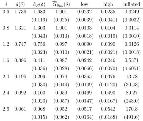
Formula (22) does not apply here so that we don’t have a natural initial sampler. But it is obvious from formulae (29) and (30) that ˆa(δ) has to be a decreasing function of δ with ˆa(1) = 1. Whence we selected a0(δ) = 1/δ for the initial sampler (other starting values such as a0(δ) = 1 work equally well but may require additional EIS iterations). Results are presented in Table 1 for values of δ ranging from 0.6 to 2.6. The two samplers used for the convergence test discussed above are the EIS sampler with ˆaR(δ) and one with
ˆ
a1(δ) = 5.ˆaR(δ) (equivalent to multiplying the variance of the EIS sampler
by five). Obviously, for δ = 1 the EIS sampler satisfies equation (9) with ˆ
aR(δ) = 1 and is perfect. While an exponential sampler is not particularly
efficient for values ofδ very different from 1, this pilot application illustrates some important points.
• The final (iterated) EIS regression coefficients ˆaR(δ) are accurate LS
estimates of ˆa(δ);
• The two variance bounds in equation (18) are always very close to one another, negating the need for solving the nonlinear LS problem in equation (15). The MC sampling variances for GS;m(δ) - obtained
by rerunning the entire EIS algorithm under different seeds - slightly exceeds these bounds. This reflects additional variance due to the fact that a(δ) is being estimated by ˆaR(δ) - see the discussion in Section 5
below.
• The two variance estimates for the convergence test are very close to one another for δ < 1, start diverging for 1 < δ < 2 (V(a;δ) remains finite but the tails of the EIS sampler are thinner than those of ϕ) and rapidly diverge for δ >2. Note also the explosion in the MC standard deviation of the inflated variance estimate. In sharp contrast, the MC standard deviations of ˆGR(δ) provide no indications of the problem.
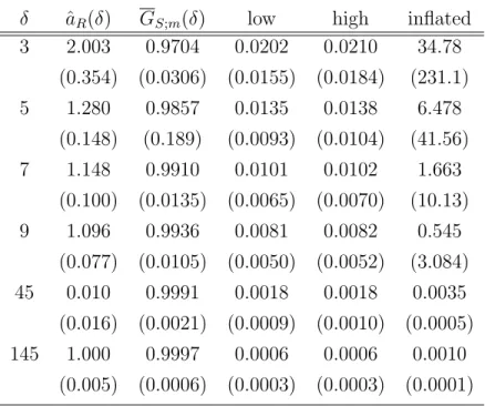
Our second pilot application considers the classical (pathological) prob-lem of approximating a Student−t density by a Normal density. Let
ϕ(x;δ) = Γ( δ+1 2 ) Γ(1 2)Γ( δ 2) · δ−2 2 −1 2 · 1 + 2x 2 δ−2 −1 2(δ+1) (33)
This particular parametrization ensures thatG(δ) = 1 and also that Varϕ(x|δ) =
0.5 for all δ >2. The family k of Gaussian kernels is parametrized as
k(x;a) = exp(−ax2) (34)
so that Varm(x|a) = (2a)−1. Note that ϕ(x;δ) converges to m(x|1) for δ →
∞. Results are presented in Table 2 and here again, highlight the high sensitivity of our convergence test to the thin tail problem. In contrast MC standard deviations for GS;m(δ) fail to detect any problem.
4
High-Dimensional EIS implementation
The EIS-LS algorithm introduced in Section 3 only applies to very low-dimensionalx’s. In higher dimensional set-ups, feasibility requires that it be
decomposed into a sequence of low-dimensional optimization problems. We now present an operational sequential implementation of EIS which, as strik-ingly illustrated by the applications discussed in Section 6 below, is applicable in very high dimensional integration problems. It exploits the fact that high-dimensional models are typically specified not as a single joint distribution but as a sequence of conditional distributions whereby latent and observable variables are generated individually (sequentially in the time dimension or in parallel in cross sections). Therefore, we now assume that there exists a natural sampling preordering partition of x into low-dimensional (typically univariate) components, say x= (x1,· · ·, xL). The functionals ϕ, g and pin
equation (8) are partitioned conformably with x into
ϕ(x;δ) = ΠL`=1(X`;δ), g(x;δ) = ΠL`=1g`(X`;δ)
(35)
p(x|δ) = ΠL`=1p`(x`|X`−1, δ) (36)
where X` = (x1,· · ·x`) and X0 denotes known initial conditions. Unknown initial conditions would be included in the x’s to be integrated in which case
X0 could be empty. Our notation highlights the fact that p constitutes a sequential (initial) sampler for x while ϕ and g do not. It also covers time series as well as cross section applications which as illustrated in Section 6 below, translate into appropriate conditional independence assumptions (and/or exclusion restrictions) in the expressions of (ϕ`, p`, g`). The EIS
sampler m(x|a) is then partitioned conformably as
m(x|a) = ΠL`=1m`(x`|X`−1, a`)
(37)
with a = (a1,· · ·, aL)∈A= ΠL`=1A`. As discussed in Section 3.1 above, EIS
approximations involve kernels instead of densities since, in particular, the integral of ϕ` w.r.t. x` is unknown. A kernel k` for m` is a function which is
proportional to m` for any given (X`−1, a`). The following notation applies
to a kernel k`, its integral χ` and the corresponding density m`:
χ`(X`−1;a`) = Z k`(X`;a`)d x` (38) m`(x`|χ`−1, a`) = k`(X`;a`) χ`(X`·1;a`) (39)
The very fact that the integrating constant χ` may and actually will
-depend on X`·1 has critical implications for our sequential EIS implemen-tation. Specifically if in line with equation (12), we aimed at approximat-ing ln ϕ`(X`;δ) by a log kernel ln k`(X`;a`), then the integrating constant
χ`(X`·1;a`) would not be accounted for. This would amount to ignoring the
fundamental sequential structure of the initial model and would inevitably produce highly inefficient overall samplers. Since, however, χ` does not
de-pend on x` and has a known analytical expression, it can be transferred
back and explicitly accounted for in the (`−1)th suboptimization problem. Specifically, this amounts to reshuffling the partitioning of m as follows:
ϕ(x;δ) m(x|a) = Π L `=1 ϕ`(X`;δ) m`(x`|X`−1, a`) (40) =χ1(X0;a1)·ΠL`=1 ϕ`(X`;δ)·χ`+1(X`;a`+1) k`(X`;a`)
withχL+1(·)≡1. The sequential implementation of EIS immediately follows from equation (40). It consists of a back-recursive sequence of optimization subproblems, whose step ` consists of approximating ln(ϕ` ·χ`+1) by lnk`.
More specifically, the backward recursion on {ˆa`(δ);` :L→1} is given by:
ˆ a`(δ) = ArgMina`,γ` 1 R R X i=1 ln ϕ`( ˜X (i) ` ;δ)·χ`+1( ˜X (i) ` ; ˆa`+1(δ)) −γ`−ln k`( ˜X (i) ` ;a`)]2·g`( ˜X (i) ` ;δ) (41)
where ˜X`(i) = (˜x(1i),· · ·,x˜(`i)) and the {x˜(`i)} denote i.i.d. trajectories drawn from the initial sampler - that is to say ˜x(`i) is drawn from p`(x`|X˜
(i)
`−1, δ). As above, we recommend deleting the weight factorg`, at least in the initial EIS
iteration(s). Note that it is critical that lnk` approximates well ln(ϕ`, χ`+1) in X`, not simply in x`. Once an EIS sequence of kernels {k`} has been
obtained, the EIS estimate ofG(δ) is computed by formula (5) under (CRN) trajectories {xˆ(1i),xˆ2(i),· · ·,xˆ(Li)} drawn from the corresponding EIS samplers
{m`}. We note that the convergence test introduced in Section 3.5 can be
applied individually to each EIS optimization subproblem, with the advan-tage that it would single out individual kernels which could be responsible for a poor global EIS approximation.
We conclude this presentation of our sequential EIS implementation with two important remarks.
First, the sequence of low dimensional optimization problem is not equiv-alent to the (unfeasible) joint optimization. In order to illustrate the implicit trade-off, let us consider the case where L= 2 andx= (x1, x2). In line with
equation (40) we can rewrite G(δ) as: G(δ) = Z ϕ1(x1;δ)[ Z ϕ2(x;δ)dx2]dx1, (42) =χ1(a1)· Z ϕ 1(x1, δ)·χ2(x1;a2) k1(x1, a1) ·h2(x1;a2, δ)·m1(x1|a1)dx1, with h2(x1;a2, δ) = Z ϕ 2(x;δ) k2(x;a2) ·m2(x2|x1, a2)dx2 (43)
The terms between brackets in the right-hand sides of equations (42) and (43) correspond to the two EIS subproblems defined in equation (21). It follows that the functionh2 is not accounted for in our sequential EIS imple-mentation. Since, however, the key to a successful EIS solution is that the ratios ϕ`χ`+1/k` be near constant, h2 itself should be near constant and its omission from the EIS optimization ought to be largely inconsequential. This heuristic justification will be fully supported by the exceptional efficiency of the EIS sequential algorithm in very high-dimensional applications such as those presented in Section 6 below.
Second, the fact that the sequential EIS algorithm runs backward could be perceived to be a significant drawback since, in particular, it requires recomputing the EIS sampler each time new dimensions of integration are added. However, such reruns are expected to be very fast since one can use as initial sampler for such a rerun the EIS sampler previously computed for the lower dimensional problem augmented by the natural sampler for the added dimensions. Under standard mixing assumptions one would expect that the impact of the added dimensions would fade out as the algorithm runs backward and that only a relatively small number of EIS subsamplers would have to be significantly adjusted.
5
Numerical and Statistical Properties of EIS
Estimates
Following equation (5), an EIS functional estimate of G(δ) has the form
GS;m(δ,ˆaR(δ)) = 1 S S X i=1 w(˜xi(δ);δ,aˆR(δ))·g(˜xi(δ), δ) (44)
where ˆaR(δ) minimizes ˆQR(a;δ) as given in equation (25) and {x˜i(δ);i: 1→
S} are i.i.d. draws fromm(x|aˆR(δ)) obtained from a fixed matrixU of CRN
by a transformation of the form given in equations (26) or (27). Therefore, ˆ
aR,{x˜i}and GS;m are all implicit functions of δ andU. The following
short-hand notation will prove useful for our subsequent analysis
GS(δ, U) =GS;m(δ,ˆaR(δ))
(45)
Note that it is a trivial matter to rerun our entire EIS algorithm under i.i.d. draws from U since it is just a matter of changing the initial seed of the random number generator. This enables us to produce i.i.d. draws from GS(δ, U) from which the following improved estimate of G(δ) obtains
together with its MC variance
GSL(δ) = 1 L L X `=1 Gs(δ,u˜`) (46) VarU (GSL(δ)) = 1 L 1 L L X `=1 (δ,u˜`)−G 2 SL(δ) (47)
That same MC simulation procedure can be used to produce estimates of the numerical accuracy of any implicit transformation of G(δ). Assume for example, that δ = (θ, y) where y is an observed sample and θ a vector of unknown parameter. Let G(δ) in equation (1) denote the corresponding likelihood function, marginalized w.r.t. a vector x of latent variables. Let
ˆ
θ(y) denote the (unfeasible) Maximum Likelihood (hereafter ML) of θ, and ˆ
θs(y, U) its ML-EIS (numerical) estimate, respectively defined as
ˆ θ(y) = Arg Maxθ ln G(θ, y) (48) ˆ θS(y, U) = Arg Maxθ ln GS(y, θ, U) (49)
As above, we can rerun under different seeds the entire EIS-ML algorithm now consisting of equations (44), (45) and (49), in order to obtain i.i.d. draws of ˆθs(y, U) from which to compute a final EIS-ML estimate of ˆθ(y) together
with its numerical covariance matrix, respectively given by ˆ θSL(y) = 1 L L X `=1 ˆ θs(y,u˜`) (50) VarU (ˆθSL(y)) = 1 L 1 L L X `=1 ˆ θ2S(y,u˜`)−θˆ2SL(y) (51)
Finally, we can also produce by MC simulation an EIS estimate of the statistical covariance matrix of ˆθ(Y) as an estimator of θ. Note that, as highlighted in Section 3.4, Y and U are independent of one another by con-struction. Therefore, we can fix U and use our (estimated) statistical model to produce draws ofY|θ- in practice, we would draw joint trajectories{x˜i,y˜i}
and only retain the ˜yi, s. The corresponding EIS estimate of the statistical
covariance matrix of ˆθ(y) is given by ˆ VarY|θ(ˆθ(Y)) = 1 L L X `=1 ˆ θ2s(˜y`, U)−θ 2 SL , with (52) θSL = 1 L L X `=1 ˆ θS(˜y`, U) (53)
In summary, once an ML-EIS program has been produced it can trivially be embedded in two independent MC simulation loops in order to compute covariance matrices for ˆθS(y, U) as a numerical estimate of ˆθ(y) and for ˆθ(y)
as a statistical estimate of θ. Similar numerical procedures apply to other classes of estimators.
We conclude this section by emphasizing the fact that our recommended practice of computing numerical and statistical covariance matrices for EIS-based estimators contrasts with the classical treatment of simulation estima-tors in the recent econometric literature. Useful references are McFadden (1989), Pakes and Pollard (1989) or, more recently, Gourieroux and Monfort (1993, 1996). In that literature, the sampling properties of simulation estima-tors are derived from the joint distribution of the observable as well as latent variables. Under appropriate conditions the (fixed S) asymptotic covariance matrix of ˆθS(y, U) equals (1 +S−1) that of ˆθ(Y). While such results
pro-vide a convenient characterization of numerical accuracy, they hide the fact that joint simulation of (Y, U) often constitutes a highly inefficient numeri-cal treatment of latent variables. As dramatinumeri-cally illustrated by the results provided in our next section, EIS treatments of latent variables which aim at drawing latent variables (near) conditionally on the observables - result in far greater relative numerical accuracy than conventional joint simulation.
6
Two High-Dimensional Pilot Applications
We now present two high-dimensional applications illustrating the high nu-merical accuracy of ML-EIS estimation for two important classes of latent
variable models: stochastic volatility and panels with unobserved heterogene-ity along both dimensions.
6.1
Stochastic Volatility
Stochastic volatility models play a central role in finance. Pioneering contri-butions are Taylor (1986), Melino and Turnbull (1990) or Duffie and Singleton (1988). It has long been recognized that natural IS, as defined in equation (2), is hopelessly inefficient - see Danielsson and Richard (1993) for a dra-matic illustration of such inefficiency. In order to illustrate the full flexibility of our EIS algorithm in this context we consider here four versions of the same baseline model. Let yt denote the daily return of a financial asset and
λt its unobserved variance (Stochastic Volatility, hereafter SV). SV models
typically consist of a stochastic equation for yt given λt and another for λt
given λt−1 (which can trivially be generalized into a higher order autoregres-sive process). Two versions of the density g(yt|λt,·) will be considered: a fat
tail Student-tdensity (S) and a thin tail Normal density (N). For the density
p(λt|λt−1,·), we shall consider in turn an Inverted-Gamma (G) density and a Lognormal density (L). These four densities are parametrized as follows:
gt1(yt|λt, θ)∝λ 1 2 t · 1 + (yt−µ) 2) λt(w−2) −12(w+1) , (54) g2t(yt|λt, θ)∝λ −1 2 t ·exp −1 2 · (yt−µ)2 λt , (55) p1t(λt|λt−1, θ)∝r 1 2ν t−1·λ −1 2(ν+2) t ·exp −rt−1 λt , (56) with rt−1 = 1 2(γ+∂λt−1) and E(λt|λt−1) = 2 v −2rt−1 =q+rλt−1 p2t(vt|vt−1, θ)∝exp − 1 2σ2(vt−q−rvt−1) 2 (57)
where vt =lnλt and θ includes the corresponding subset of the parameters
(q, r, σ, µ, ω, ν). We shall consider here the four pairwise combinations of qt
and pt, respectively denoted SG, SL, NG and NL, but shall only detail the
sequential EIS implementation for the SG version since the other versions only require fairly obvious modifications of the auxiliary regressions.
Since p1
t belongs to the exponential family of distributions and is closed
accordingly the class Kt as consulting of products of two I-G kernels, one
consisting of all I-G factors in ϕt = gt1p1t and the other designed to best
approximate the remainder. Since the latter only depends on λt, we shall
select the following forms for the EIS kernel kt and its integrating constant
χt: kt(λ(t), at)∝ r 1 2ν t−1·λ −1 2(ν+3) t exp(− rt−1 λt ) · λ−bt t ·exp(− ct λt ) (58) χt(λt−1, at)∝r 1 2ν t−1·(rt−1+ct)− 1 2(ν+1)−bt (59)
with a0t = (bt ct). Note the inclusion of rt−1, which only depends on λt−1, in the expression for kt. It provides a convenient way of making sure that
rt−1 will be accounted for in the period t−1 EIS auxiliary regression. By construction, all terms included between the first two brackets in equation (58) belong to both ϕt and kt. Therefore, they cancel out in the auxiliary
EIS regressions which simplify into the following OLS regressions: Dependent variables: ln χt+1(λt,ˆat+1)− 1 2(w+ 1)· ln 1 + (yt−µ) 2 λt(w−2)
Regressors: ln λt and λ−t1 (plus one intercept)
(60)
Equations (58) to (60) are all we need to apply the sequential EIS algorithm described in Section 4. As discussed above, we rerun EIS under a fixed set of CRN’s for each evaluation of the likelihood function. The computing time required for a very large number of inversion of the IG distribution function is considerably reduced by the initial construction of a high-accuracy bivariate interpolation table (U and degrees of freedom) for the IG inverse distribution function. For the purpose of illustration we computed ML-EIS estimates for a sample consisting of 1,447 observations of IBM daily stock price changes for the period 1/9/82-3/31/87. As indicated by the results reported in the SG row of Table 3, ML-EIS estimates are numerically extremely accurate even with as little as R = S = 10 MC draws (note, in particular, that the ratios between numerical and statistical standard deviations is much smaller than the classical S−1/2 ratio). Table 3 also reports results for the SL, NG and NL cases.
Total computing time for a full ML optimization (using a simplex algo-rithm which is extremely robust for this type of applications) is of the order of 45 seconds on a 750 MHZ UNIX server (and about 15 seconds for the
faster NL version). The high persistence with values of r in the 0.95-0.98 range is typical of SV models. We note that the Lognormal density for λt
is qualitatively better identified than its IG counterpart. Actually, it can be shown that the high-value of ˆr also requires a high value for ˆν in order to match the sample (stationary) variation coefficient ofλtwhich is of the order
of 0.4.
The high numerical accuracy of EIS in the context of SV models results from the facts that: (i) The observation {yt} are very informative on the
underlying latent process {λt} and EIS is designed precisely to take full
ad-vantage of such situations; (ii) A total of 2T = 2,894 auxiliary parameters were used to construct the EIS sampler. Such high accuracy has been fully confirmed by recent applications of EIS to a wide range of SV models (uni-variate, bi(uni-variate, two factors, semi-parametric versions) in dimensions up to 8,000+. See Liesenfeld and Richard (2003a, b). Comparisons with alterna-tive numerical evaluations of SV models are found in Liesenfeld and Richard (2003c) and Bauwens and Hautsch (2003). The combination of high numeri-cal accuracy and ease of implementation of EIS appears to be unmatched in that class of models.
6.2
Logit with Unobserved Heterogeneity
It is commonly held in the econometric literature that ML estimation of panel data models with unobserved random heterogeneity along both dimensions is unfeasible - see e.g. the comments in McFadden (1989). This has led to the development of alternative though statistically less efficient simulation based estimation techniques. See Lerman and Manski (1981), McFadden (1989), Pakes and Pollard (1989) or B¨orsch-Supan and Hajivassiliou (1990). See also Gourieroux and Monfort (1993) for a survey or Gourieroux and Monfort (1996) for an in-depth analysis of simulation based inference techniques.
In this section, we demonstrate that contrary to common beliefs, highly accurate numerical evaluation of the likelihood function of such panel data models is fully operational under EIS. Consider a model consisting of a logit for the observable yit ∈ {0,1} conditionally on the random effects αi and
λt, independent normal distributions for the α’s and a multivariate normal
distribution for the λ’s. Let α0 = (α1· · ·αN), λ0 = (λ1· · ·λT), y0 = (yit;i :
1 →N, t : 1 →T) and δ = (y, θ) where θ regroups all unknown parameters in the model. Let xit denote a vector of exogenous variables. The likelihood
function is of the form given by equation (1) together with g(α, λ, δ) =g0(λ, δ)·ΠNi=1gi(αi, λ, δ) (61) with g0(λ, δ)≡1 and gi(αi, λi, δ) = ΠTt=1 [exp(vit]yit 1 + exp(vit) (62) vit =β0xit+αi+λt (63) p(α, λ|δ) =p0(λ|θ)·ΠNi=1pi(αi|θ) (64) p0(λ|θ)∝ |Hθ| 1 2 exp−1 2λ 0 Hθλ (65) pi(αi|θ)∝σα−1exp −1 2 α i σα 2 (66)
It is implicitly assumed here that N >> T as commonly the case. For
T >> N we would permute the α’s and λ’s in all factorizations. Extensions such as exchangeable α’s are trivially handled by conditioning the densities
pi in equation (66) on a common factor α0 and adding an additional density for α0. Notationally this would amount to incorporating α0 into λ.
It is obvious from equations (61) to (66) that we should partition EIS samplers conformably with p in equation (64), with the critical extension that the αi’s are now to be independent conditionally on λ in order to fully
account for the (posterior) dependence between α and λ as induced by g. Specifically, we select for the αi’s conditionally independent kernels of the
form ln ki(αi, λ, ai) =− 1 2 2b0ivi+v0iCivi+ α i σα 2 (67) with vi =Xiβ+λ+αie, Xi0 = (xi,· · ·, xiT), λ0 = (λ1· · ·λT), e0 = (1· · ·1), bi ∈RT, Ci = Diag (ci), ci =
Cie∈RT+ and ai = (bici). It turns out that the constraintsci >0 never bind
and can safely be ignored. Note that the integrating constant χi associated
with ki only depends upon (λ, ai), not upon the other αj’s. In order to
facilitate subsequent EIS integration w.r.t. λ, ln kiis rewritten as a quadratic
form in λ and is given by
ln χi(λ, ai)∝ − 1 2 `0iCi`i+ 2`0ibi− α i σi 2 (68)
with `i =λ+Xiβ, σi−2 = σ −2 α +c 0 ie and αi =−σ2i(` 0 ici+b0ie) (69)
In summary, the EIS auxiliary GLS regressions for the αi’s consist of
regress-ing ln gi on the 2T regressions {(vit, vit2);t : 1 → T} with an intercept and
weights git (OLS for the first EIS iteration). Under EIS sampling and
con-ditionally on λ, the αi’s are independently normally distributed with means
αi and variances σi2.
As for λ, we note that ϕ0 = g0p0 and {χi;i : 1 → N} all are in the
forms of Gaussian kernels. Therefore, a perfect EIS sampler for λ obtains immediately by combining together the N + 1 quadratic forms in equations (65) and (68) - providing a remarkable example of “perfect fit” in the sense of equation (9). Rearranging terms in the usual way, we find that
m0(λ|a0)∝ |A| 1 2 exp −1 2(λ−µ) 0 A(λ−µ) (70)
with a00 = (µ0, vec0A) and
A=H0+ N X i=1 (Ci−σi2cic0i) (71) µ=−A−1 N X i=1 CiXiβ+bi−σi2(c 0 iXiβ+b0ie)ci (72)
This completes the description of the EIS algorithm for this application. Note the very large number of auxiliary parameters (of the order of 2T N) used to produce the EIS approximation to the actual posterior density of (α, λ). A caveat applies before we present numerical results. As in Section 6.1 we shall aim at running the auxiliary EIS regressions under relatively small numbers of MC draws (of the order of three times the number of regressions). As the vit’s all depend on αi, occasional bad draws can generate very high
multicollinearity in the auxiliary regressions and even crash the EIS algorithm (Production of the results reported in Table 4 required several millions of EIS regressions!). We were able to completely eliminate the problem by introducing a small amount of shrinkage in the auxiliary EIS regressions. Specifically, we used a second order Taylor Series Expansion (hereafter TSE) of gi aroundαi = λt = 0 in order to produced exact restrictions for ai. Let
these restrictions be written as
ai =Riδi+qi
where δi ∈ R` with ` < 2T denotes free regression coefficients and (Riqi)
is a 2T · (` + 1) matrix of known constants (which actually depend upon
{xit, yit);t : 1 → T} and β which are all included in δ). An unconstrained
EIS OLS estimator of the form ˆai =G−i 1hi is then replaced by the shrinkage
estimator
˜
ai = (Gi+κMi)−1(Ri+κMiqi)
(74)
with Mi =I2T −Ri(R0iRi)−1R0i. This shrinkage option completely eliminates
unwanted interruptions of the EIS algorithm at virtually no loss of EIS effi-ciency even with very low values of κ (0.01 or less in the application which follows).
In order to illustrate the impressive numerical performance of EIS within this class of models, we generated a fictitious sample of size T = 15 and
N = 1,000, with no exogeneous variables and a stationary AR(1) process for λ with autocorrelation coefficient ρ and stationary variance σ2λ. The parameters true values were set equal toσα =σλ = 0.3 andρ= 0.5, implying
a relatively moderate amount of heterogeneity (results derived under different values produce similar qualitative results). The number of regressors in each EIS auxiliary regression equals 30 (plus one intercept). We usedR =S = 100 MC draws and 3 EIS iterations.
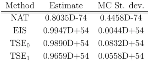
In Table 4.1 we report MC estimates of the likelihood function at the parameter true values under the natural sampler (NAT), as defined by equa-tions (64) to (66), the EIS sampler (EIS), the sampler obtained by TSE of the gi, s aroundαi =λi = 0 (TSE0) and an (unfeasible) sampler obtained by
TSE of the gi, s around the true values of αi and λt, which we had initially
stored (TSE1). TSE1 is closest in spirit to the Laplace approximations pro-posed by Tierney and Kadane (1986). Obviously, in practice the α’s andλ’s would have to be estimated first which would result in increased numerical inefficiency. The results in Table 4.1 illustrate the clear superiority of our EIS global approximations relative to TSE local ones. The results also indi-cates that the problem associated with the natural sampler in this context is one of enormous downward bias more than variance. Actually, this result is not surprising. Assume an individual αi draw from pi has a probability
0.75 of hitting the region of importance. The probability that N = 1,000 independent draws jointly hit the region of importance is then of the order of 10−124.
Finally, in order to illustrate the performance of EIS within an inferen-tial context, we computed ML-EIS estimates of θ. Full optimization using a
simplex algorithm requires of the order of 50 EIS likelihood evaluations for a computing time of the order of 1 minute on our 750 MHZ UNIX worksta-tion. As in Section 6.1, numerical as well as statistical standard deviations were produced using 20 replications of the EIS-ML optimization (under the estimated values). The results are reported in Table 4.2. Note here again the impressive numerical accuracy of the results. The particular sample we used appears to have produced a borderline value for ˆρ(Note, however, that we only have T = 15 periods, that is to say only 15 latent λt’s to identify
ρ). In order to verify that the low value of ˆρ was due to that particular sample and not to an inherent EIS-ML problem, we ran 50 MC replications of our algorithm under the parameter true values. The corresponding sta-tistical means and standard deviations equal (0.2922, 0.2965, 0.4726) and (0.0627, 0.0287, 0.1850), respectively. The (EIS) ML estimators are clearly statistically well-behaved.
This EIS-ML algorithm has recently been successfully applied by Liesen-feld and Richard (2004) to a dynamic logit model for the union participation decision of young men. The data (N = 545, T = 8) were taken from Vella and Verbeek (1998) who estimated the model under random individual effects and fixed time effects. Randomizing both heterogeneity components enable Liesenfeld and Richard to qualify their relative impact on agents’ decisions. They find that the dynamic of the union participation decision is dominated by individual heterogeneity.
7
Conclusion
We proposed an operational recursive Least Square algorithm to construct (very) high dimensional Importance Samplers. In contrast with current pro-cedures, which are mostly based upon local approximations of the integrand, our algorithm explicitly minimizes the variance of the MC-IS estimate in order to produce a global approximation to the posterior density of the vari-ables to be integrated out. Our algorithm’s performance in high-dimensional latent variables models is unparalleled, as illustrated in the context of two important classes of models in the modern econometric literature. Its success appears to result from a combination of three factors: (1) The availability of full sequential factorizations which reduce the optimization problem to an operational sequence of low-dimensional Least Squares problems, (2) The use of very large number of auxiliary parameters, typically a multiple of the
sample size in order to produce very good global fit between the integrand and the importance sampler; and (3), last but not least, the fact that the posterior densities of the latent variables appear to be very well-conditioned in the applications we have considered.
EIS is not meant to substitute for other methods under all circumstances. In particular, Monte Carlo Markov Chain (MCMC) algorithms appear to be well adapted to Bayesian applications when posterior densities of the para-meters are ill-behaved and/or cannot be conveniently sequentially factorized as required for EIS. But neither do we believe that MCMC can be indis-criminately applied across the board. Actually, we believe the two methods can be complementary and we are currently investigating the possibility of combining both to conduct operational full Bayesian analysis of (dynamic) latent variable models, such as the ones we analyzed here within a classical ML framework.
Acknowledgements: We are particularly indebted to Roman Liesenfeld
who, together with the first author, has developed several highly successful applications of EIS. This experience has led to major improvements of the present paper. Our work has been supported by the National Science Foun-dation (Grant SES-9223365).
8
References
Bauwens, L., and Hautsch, N. (2003), “Stochastic Conditional Intensity Processes”, working paper available at http://www.econ.au.dk/ec2bologna/papers /lb sci.pdf.
B¨orsch-Supan, A. and Hajivassiliou, V. (1990), “Smooth Unbiased Multivari-ate Probability Simulation for Maximum Likelihood Estimation of Limited Dependent Variable Models,” Cowles Foundation discussion paper no. 960, Yale University.
Danielsson, J. and Richard, J.F. (1993), “Accelerated Gaussian Importance Sampler with Applications to Dynamic Latent Variable Models,” Journal of Applied Econometrics 8, 153-173.
DeGroot, M.H. (1970), “Optimal Statistical Decisions,” New York: McGraw-Hill.
Devroye, L. (1986), “Non-Uniform Random Variate Generation,” New York: Springer–Verlag.
Duffie, D., and Singleton, K.J. (1988), “Simulated Moment Estimation of Markov Models of Asset Prices,” Stanford University mimeo.
Durbin, J., and Koopmans, S.J. (1997), “Monte Carlo Maximum Likelihood Estimation for non-Gaussian State Space Models,” Biometrika, 84, 669-684.
Evans, M. (1991),“Adaptative Importance Sampling and Chaining,” Con-temporary Mathematics (Statistical Multiple Integration), 115, 137-142. Fishman, G.S. (1996), “Monte Carlo Concepts, Algorithms, and Applica-tions,” New York: Springer-Verlag.
Geweke, J. (1989), “Bayesian Inference in Econometric Models Using Monte Carlo Integration,” Econometrica, 57, 1317-1339. - -(1996), “Monte Carlo Simulation and Numerical Integration,” in The Handbook of Computational Economics, Vol. 1., eds. H. Amman, D. Kendrick, J. and Rust, Amsterdam: North Holland.
Gourieroux, C., and Monfort, A. (1993), “Simulation Based Inference: A Survey with Special Reference to Panel Data Models,”The Journal of Econo-metrics, 59, 5-33.
- -(1996), “Simulation Based Econometric Methods,” CORE Lecture Series, Oxford: Oxford University Press.
Hammersley, J.M., and Handscomb, D. (1964), “Monte Carlo Methods,” London: Methuen.
Kahn, H., and Marshall, A. (1953), “Methods of Reducing Sample Size in Monte Carlo Computations,” Journal of the Operations Research Society of America, 1, 263-278.
Koopman, S. J., and Shephard, N. (2004), ”Estimating the Likelihood of the Stochastic Volatility Model: Testing the Assumptions Behind Importance Sampling,” Free University Amersterdam mimeo.
Lerman, S., and Manski, C. (1981), “On the Use of Simulated Frequencies to Approximate Choice Probability,” inStructural Analysis of Discrete Data with Econometric Applications, Chap. 7, eds. C. Manski and D. McFadden, Cambridge, MIT Press,
Liesenfeld, R., and Richard, J.F. (2003a), “Monte Carlo Methods and Bayesian Computation: Importance Sampling,” in The International Encyclopedia of the Social and Behavioral Sciences, 10000-10004, eds. N. J. Smelsev and P. B. Baltes, Oxford: Elsevier-Science.
- -(2003b), “Univariate and Multivariate Volatility Models: Estimation and Diagnostics,” The Journal of Empirical Finance, 10, 505-531.
- -(2003c), “Estimation of Dynamic Bivariate Mixture Models: Comments on Watanabe,” The Journal of Business and Economic Statistics, 21, 570-576. - -(2004), “Simulation Techniques for Panels: Efficient Importance Sam-pling,” forthcoming in the Econometrics of Panel Data, A Handbook of the Theory eds. L. Matyas and P. Seveitse, 3rd edition, Boston: Kluwer.
Madras, N., and Piccioni, M. (1994), “Importance Sampling for Families of Distributions,” The Annals of Applied Probability, 9, 1202-1225.
McFadden, D. (1989), “A Method of Simulated Moments for Estimation of Discrete Response Models Without Numerical Integration,” Econometrica, 57, 995-1026.
Melino, A., and Turnbull, S. (1990), “Pricing Foreign Currency Options with Stochastic Volatility,” Journal of Econometrics, 45, 239-265.
Owen, A., and Zhou, Y. (2000), “Safe and Effective Importance Sampling,”
Journal of the American Statistical Association, 95, 135-143.
Pakes, A., and Pollard, D. (1989), “Simulation and the Asymptotics of Op-timization Estimators,” Econometrica, 57, 1027-1057.
Stern, S. (1997), “Simulation-Based Estimators,” Journal of Economic Lit-erature, 35, 2006-2039.
Taylor, S. (1986), “Modeling Financial Time Series,” Chichaster: John Wiley. Tierney, L., and Kadane, J.B. (1986), “Accurate Approximations for Poste-rior Moments and Marginal Densities,” Journal of the American Statistical Association, 81, 82-86.
Trotter, H.F., and Tukey, J.W. (1956), “Conditional Monte Carlo for Normal Samples,” in Symposium on Monte Carlo Methods, ed. H.A. Mayer, New York: John Wiley.
Vella, F., and Verbeek, M. (1998), “Whose Wages Do Unions Raise? A Dynamic Model of Unionism and Wage Rate Determination for Young Men,”
Table 1: EIS Results for ϕ in Equation (29)
Variance Estimates
δ aˆ(δ) ˆaR(δ) GS;m(δ) low high inflated
0.6 1.736 1.683 1.001 0.0232 0.0235 0.0249 (0.119) (0.025) (0.0039) (0.0041) (0.0032) 0.8 1.321 1.303 1.001 0.0103 0.0104 0.0114 (0.043) (0.013) (0.0018) (0.0019) (0.0010) 1.2 0.747 0.756 0.997 0.0090 0.0090 0.0126 (0.023) (0.010) (0.0021) (0.0021) (0.0018) 1.6 0.396 0.411 0.987 0.0242 0.0246 0.5371 (0.036) (0.028) (0.0066) (0.0070) (0.6051) 2.0 0.196 0.209 0.974 0.0365 0.0376 13.78 (0.030) (0.044) (0.0109) (0.0120) (30.43) 2.4 0.092 0.100 0.959 0.0469 0.0490 89.27 (0.020) (0.057) (0.0147) (0.0167) (243.0) 2.6 0.061 0.068 0.952 0.0517 0.0542 170.8 (0.015) (0.062) (0.0164) (0.0188) (491.6) Relevant formulae: ˆ
a(δ) : Population EIS Coefficient; Formula (32) ˆ
aR(δ) : Mean EIS-OLS Coefficient; Formula (25) - Unweighted
GS;m(δ) : Mean EIS-Estimate of G(δ) = 1; Formula (5)
Low: Lower Bound h[Q(ˆaR(δ) :δ)]; Formula (18)
High: Upper Bound V(ˆaR(δ);δ); Formula (18)
Inflated: V(0.2ˆaR(δ);δ); Formula (28)
Additional Details:
Number of MC Draws: R = S = 100; Number of EIS Iterations: 15
(Needed for δ = 2.6); Numbers in Parentheses are MC standard Deviations based upon 50 Replications of EIS
Table 2: EIS Results for Student t Density - Equation (33)
Variance Estimates
δ ˆaR(δ) GS;m(δ) low high inflated
3 2.003 0.9704 0.0202 0.0210 34.78 (0.354) (0.0306) (0.0155) (0.0184) (231.1) 5 1.280 0.9857 0.0135 0.0138 6.478 (0.148) (0.189) (0.0093) (0.0104) (41.56) 7 1.148 0.9910 0.0101 0.0102 1.663 (0.100) (0.0135) (0.0065) (0.0070) (10.13) 9 1.096 0.9936 0.0081 0.0082 0.545 (0.077) (0.0105) (0.0050) (0.0052) (3.084) 45 0.010 0.9991 0.0018 0.0018 0.0035 (0.016) (0.0021) (0.0009) (0.0010) (0.0005) 145 1.000 0.9997 0.0006 0.0006 0.0010 (0.005) (0.0006) (0.0003) (0.0003) (0.0001)
Relevant Formulae and Details: Same as for Table 1
Table 3: Stochastic Volatility; EIS-ML Estimates (IBM Data) ˆ q rˆ σˆ µˆ ωˆ νˆ ln L(ˆθ, y)×10−4 0.0526 0.9698 - 0.0518 21.63 226.55 -0.10869 SG (0.0003) (0.0002) (0.0005) (0.18) (0.62) (0.00001) [0.0275] [0.0184] [0.0216] [13.91] [61.89] 0.0742 0.9568 - 0.0503 - 133.83 -0.10887 NG (0.0008) (0.0004) (0.0004) (1.85) (0.00001) [0.0280] [0.0177] [0.0205] [62.13] 0.0116 0.9763 0.0788 0.0535 19.82 - -0.10864 SL (0.0001) (0.0002) (0.0005) (0.0002) (0.09) (0.00000+) [0.0110] [0.0177] [0.0261] [0.0239] [11.13] 0.0197 0.9574 0.1204 0.0514 - - -0.10883 NL (0.0002) (0.0004) (0.0006) (0.0005) (0.00000+) [0.0136] [0.0315] [0.0311] [0.0234]
Notes: Number of MC Draws: R = S = 10; Three EIS Iterations;
Nu-merical () and Statistical [] Standard Deviations based upon 20 MC Repli-cations
Table 4.1: Logit: EIS Estimate of L(θ0;y)
Method Estimate MC St. dev.
NAT 0.8035D-74 0.4458D-74
EIS 0.9947D+54 0.0044D+54
TSE0 0.9890D+54 0.0832D+54
TSE1 0.9659D+54 0.0558D+54
Note: Proportionality Constants Were Ignored
Table 4.2: Logit; ML-EIS Estimates
ˆ
σα σˆλ ρˆ L(ˆθ;y)
0.2704 0.2972 0.2683 0.1610D+55
(0.0004) (0.0003) (0.0013) (0.0004D+55) [0.0482] [0.0226] [0.1828]
Notes: Sample Size: N = 1,000 and T = 15;
Three EIS Iterations; Number of MC Draws:
![Table 3: Stochastic Volatility; EIS-ML Estimates (IBM Data) ˆq r ˆ σˆ µˆ ωˆ ν ˆ ln L(ˆ θ, y) × 10 −4 0.0526 0.9698 - 0.0518 21.63 226.55 -0.10869 SG (0.0003) (0.0002) (0.0005) (0.18) (0.62) (0.00001) [0.0275] [0.0184] [0.0216] [13.91] [61.89] 0.0742 0.9568](https://thumb-us.123doks.com/thumbv2/123dok_us/1452323.2694402/32.918.195.838.227.613/table-stochastic-volatility-eis-estimates-ibm-data-σˆ.webp)