Software packages performance evaluation of basic radar signal processing techniques

University

of

Cape

Town

basic radar signal processing techniques

Presented by: Xavier Frantz

Prepared for:

Associate Professor Daniel O’Hagan Dept. of Electrical Engineering

University of Cape Town

Submitted to the Department of Electrical Engineering at the University of Cape Town in partial fulfilment of the academhic requirements for a Master of Engineering

specialising in Radar and Electronic Defence

University of Cape Town

quotation from it or information derived from it is to be

published without full acknowledgement of the source.

The thesis is to be used for private study or

non-commercial research purposes only.

Published by the University of Cape Town (UCT) in terms

of the non-exclusive license granted to UCT by the author.

I know the meaning of plagiarism and declare that all the work in the document, save for that which is properly acknowledged, is my own. This thesis/dissertation has been submitted to the Turnitin module (or equivalent similarity and originality checking soft-ware) and I confirm that my supervisor has seen my report and any concerns revealed by such have been resolved with my supervisor.

Signature: X. Frantz

I would like to thank the following people who helped with the completion of this project:

Darryn Jordan, for assisting with the implementation of pulse compression and Doppler processing algorithms.

Francois Schoken and Lerato Mohapi, for being available to brainstorm ideas for perfor-mance analysis.

Colleagues in the RRSG Radar Lab, for helping with setting up equipment, sharing resources and perfecting the implementation of algorithms.

My supervisor, Professor Daniel O’Hagan for patience and guidance during the comple-tion of the project.

My family, for constant encouragement and motivation.

I would like to thank ARMSCOR and the CSIR for their generous funding of my studies.

This dissertation presents a radar signal processing infrastructure implemented on script-ing language platforms. The main goal is to determine if any open source scripted pack-ages are appropriate for radar signal processing and if it is worthwhile purchasing the more expensive MATLAB, commonly used in industry. Some of the most common radar signal processing techniques were considered, such as pulse compression, Doppler processing and adaptive filtering for interference suppression. The scripting languages investigated were the proprietary MATLAB, as well as open source alternatives such as Octave, Scilab, Python and Julia.

While the experiments were conducted, it was decided that the implementations should have algorithmic fairness across the various software packages. The first experiment was loop based pulse compression and Doppler processing algorithms, where Julia and Python outperformed the rest. A further analysis was completed by using vectors to index matrices instead of loops, where possible. This saw a significant improvement in all of the languages for Doppler processing implementations. Although Julia performed extremely well in terms of speed, it utilized the most memory for the processing techniques. This was due to its garbage collector not automatically clearing the memory heap when required. The adaptive LMS (least mean squares) filter designs were a different form of analysis, as a vector of data was required instead of a matrix of data. When processing a vector or one dimensional array of data, Julia outperformed the rest of the software packages significantly, approximately a 10 times speed improvement.

The experiments indicated that Python performed satisfactorily in terms of speed and memory utilization. Physical RAM of computer systems is, however, constantly improv-ing, which will mitigate the memory issue for Julia. Overall, Julia is the best open source software package to use, as its syntax is similar to MATLAB compared with Python, and it is improving rapidly as Julia developers are constantly updating it. Other disadvantage of Python is that the mathematical signal processing is an add-on realized by modules such as NumPy.

1 Introduction 1

1.1 Objectives of this study . . . 2

1.1.1 Problems to be investigated . . . 2

1.1.2 Purpose of the study . . . 2

1.2 Scope and limitations . . . 2

1.3 Plan of development . . . 3 2 Literature review 4 2.1 Radar theory . . . 4 2.1.1 Radar signals . . . 4 2.2 RSP techniques . . . 6 2.2.1 NetRAD data . . . 6 2.2.2 Matched filter . . . 7 2.2.3 Pulse compression . . . 8 2.2.4 Doppler processing . . . 10

2.3 Programming languages . . . 14 2.3.1 MATLAB . . . 15 2.3.2 Julia . . . 15 2.3.3 Scilab . . . 15 2.3.4 Octave . . . 16 2.3.5 Python . . . 16

2.3.6 Additional features for interpreted languages . . . 17

2.3.7 Memory principles . . . 20

2.3.8 FFT library . . . 23

2.3.9 Floating point operations per second (FLOPS) . . . 24

3 Implementation of radar signal processing (RSP) techniques 26 3.1 Fairness . . . 26

3.2 Pulse compression implementation . . . 27

3.3 Doppler processing implementation . . . 29

3.4 Adaptive LMS filter implementation . . . 31

4 Results and discussion 36 4.1 Performance of RSP algorithm designs . . . 37

4.2 FLOPS for different RSP algorithms . . . 46

4.2.1 FLOPS for pulse compression algorithm design . . . 46

4.2.2 FLOPS for Doppler processing algorithm design . . . 48

4.3 Memory handling for pulse compression and Doppler processing . . . 50

4.4 Performance of adaptive LMS filter algorithm design . . . 53

5 Conclusions and recommendations 58 5.1 Improved performance with spatial locality . . . 58

5.2 Adequate performance of pulse compression . . . 58

5.3 Lack of JIT during Doppler processing for Octave and Scilab . . . 59

5.4 Impact of large vectors on adaptive LMS filter design . . . 60

5.5 Impact of memory utilization on various language packages . . . 60

5.6 Lack of implicit parallelism in Scilab . . . 60

5.7 Suitable alternatives to MATLAB . . . 61

5.8 Recommendations . . . 61

A Additional Procedures 62 A.1 Changing BLAS/LAPACK libraries for Scilab . . . 62

A.2 FFTW procedures . . . 62

2.1 Pulse train taken from adaptive filters applied on radar signals [1] . . . . 5

2.2 NetRAD dataset structure . . . 7

2.3 An overview of matched filtering in the frequency domain using fast convo-lution, taken from NextLook a lightweight, real-time quick look processor for NeXtRAD [2] . . . 8

2.4 Reference chirp used for transmission during NetRAD trial . . . 9

2.5 Applying pulse compression on NetRAD dataset structure . . . 9

2.6 Applying Doppler processing on a pulse compressed data set, where an oval represents a CPI . . . 11

2.7 Block diagram of an adaptive LMS filter taken from [3] . . . 12

2.8 Demonstration of spatial locality of a matrix of data. . . 23

3.1 Algorithm design for pulse compression . . . 28

3.2 RTI plot before and after pulse compression . . . 29

3.3 Algorithm design for Doppler processing . . . 30

3.4 Range and amplitude of Doppler frequencies at different range bins . . . 31

4.1 Time taken for pulse compression . . . 38

4.2 Time taken for pulse compression with different indices . . . 38

4.3 Vectorization implementation for pulse compression . . . 39

4.4 Time taken for pulse compression in Scilab with different BLAS/LAPACK libraries . . . 41

4.5 Time taken for Doppler processing . . . 42

4.6 Time taken for Doppler processing with different indices . . . 43

4.7 Vectorized implementation for Doppler processing . . . 44

4.8 Time taken for Doppler processing in Scilab with different BLAS/LAPACK libraries . . . 45

4.9 FLOPS for pulse compression . . . 48

4.10 FLOPS for Doppler processing . . . 49

4.11 Memory usage during pulse compression and Doppler processing for vari-ous language packages . . . 51

4.12 Memory utilized during Doppler processing when only necessary variables used . . . 53

4.13 Time taken per iteration for LMS processing on a fixed sized data set . . 55

4.14 Time taken for LMS processing for varied dataset sizes . . . 56

4.15 Time taken for LMS algorithm in Scilab with different BLAS/LAPACK libraries . . . 57

2.1 Default BLAS libraries used for different packages . . . 20

2.2 Basic number of operations used in RSP algorithms . . . 25

3.1 Fixed frequency signal parameters . . . 34

4.1 Standard specifications used during pulse compression and Doppler pro-cessing . . . 37

4.2 Hardware specification used for the computation of the RSP techniques . 37

4.3 Floating point operations used in pulse compression . . . 47

4.4 Floating point operations used in pulse compression . . . 49

4.5 Expected RAM utilized after pulse compression and Doppler processing were completed . . . 52

ADC Analogue-to-digital converter

ATLAS Automatically tuned linear algebra software

BLAS Basic linear algebra subprograms

CPI Coherent processing interval

CPU Central processing unit

DFT Discrete Fourier transform

FFT Fast Fourier transform

FLOPs Floating point operations

FLOPS Floating point operations per second

JIT Just-in-time

LAPACK Linear Algebra PACKage

LFM Linear frequency modulated

LMS Least mean squares

MKL Math kernal library

MSE Mean square error

NetRAD Netted Radar

OpenBLAS Open source basic linear algebra subprograms

PRF Pulse repitition frequency

PRI Pulse repitition interval

RAM Random-access memory

RefBLAS Reference basic linear algebra subprograms

RF Radio frequency

RSP Radar signal processing

RTI Range-time intensity

Introduction

The signal processor will take the raw radar data from the receiver, and perform a number of common signal processing operations on the data. These include pulse compression, Doppler processing and adaptive filtering. When performing the above algorithms, op-erations such as correlation, fast Fourier transforms (FFT) and matrix-vector algebraic operations are typically required [4].

Scientific computing is typically used for designing radar signal processing (RSP) so-lutions. Using compiled languages like C++ for processing will be time consuming as development time is longer. Its syntax is not simple; libraries have to be integrated manually or own functions have to be written, and memory has to be handled manually. Interpreted languages are much simpler and easier for engineers to use. Syntax is almost like writing mathematical expressions on paper and memory handling is automatic. The most common interpreted language used in research and industry is MATLAB. However, it is costly and extra funding would be needed for purchasing additional toolboxes. There is, therefore, a need for suitable open source alternatives to MATLAB that can provide acceptable, or even superior, performance.

1.1

Objectives of this study

1.1.1

Problems to be investigated

The main problem to be investigated in this study is the fair comparison of different scripted language packages, in the context of common RSP operations. The objectives of this report are to:

• design RSP algorithms in such a manner that performance is not decremented, but still gives algorithmic fairness across various language packages;

• compare scripting language platforms in terms of memory usage and execution time;

• draw conclusions to determine which open source software packages are viable for RSP; and

• recommend strategies to improve performance for all of the language packages such that further comparisons can be made.

1.1.2

Purpose of the study

The main purpose is to determine which of the several scripted languages are appropriate for RSP. In engineering, MATLAB is widely used in research and industry to design RSP techniques. Therefore, a requirement is to determine how open source software packages compare with the more accomplished and expensive MATLAB, as well as which of the open source packages would be recommended for various RSP techniques.

1.2

Scope and limitations

This report is limited to the implementation of pulse compression, Doppler processing and adaptive filter algorithms in MATLAB, Julia, Python, Octave and Scilab. The algorithms are designed in such a way that they can be used in various other radar applications besides the datasets used in these experiments.

• A fair algorithmic comparison was made across all of the software packages. Firstly, a loop based algorithm was written, implying that code was not written for maxi-mum performance for each language package. Secondly, code was optimized where possible in order to give faster execution time. In both scenarios, performance was measured for identical algorithmic implementation and code patterns, correspond-ing to each software package.

• Memory utilization analysis was only considered for the pulse compression and Doppler processing algorithms, because Netted Radar (NetRAD) datasets consume large amounts of memory. The dataset used for the adaptive LMS processing algo-rithms was approximately 6 megabytes (MB), for which it was not worthwhile to do a thorough memory analysis. It was decided to avoid redundancy as memory would be handled in the same way as in large datasets.

• The default linear algebra libraries were used for all the software packages, with only Scilab’s linear algebra libraries being altered for analysis and clarification purposes.

1.3

Plan of development

The rest of the report is organized in the following way:

Chapter 2 provides a literature review of the basics of radar, different RSP techniques, and software packages used in the study. It also describes important techniques that must be considered when implementing different RSP algorithms on the different language packages.

In Chapter 3 the manner in which the RSP algorithms were designed is described in detail.

Chapter 4 describes how the RSP algorithms were executed. Performance results are presented for all three RSP algorithms across all investigated software platforms, after which an analysis and comparison will follow.

Chapter 5 presents the conclusions based on the progression of the study and discusses which software packages are suitable for RSP design. Chapter 5 also has a list of recom-mendations that can be used for future work to build on the results of this study.

Literature review

2.1

Radar theory

RADAR is an acronym for radio detection and ranging. It’s two most basic functions are to detect an object and to determine it’s distance from the radar system. Radar systems have improved over the years, with the ability to track, identify, and image detected targets. A radar system typically transmits radio frequency (RF) electromagnetic (EM) waves towards a region of interest. In this region of interest, the EM waves are reflected from the objects, creating echoes. These echoes are received by the radar system and are processed to determine important information about the target [4].

2.1.1

Radar signals

In this investigation, pulsed radar systems were considered. For a pulsed radar system, radar signals have to be defined. A radar signal can be described by three important characteristics: pulse repetition interval, pulse width and carrier frequency. Radar signals consists of a train of short pulses. The pulse width (TP W) is the duration time of a pulse

and decides the bandwidth and range resolution. Pulse repetition interval (TP RI) is the

time between the beginning of one pulse and the start of the next pulse and can be designed to avoid Doppler and range ambiguities [1]. A typical envelope of a radar signal pulse train is depicted in Figure 2.1, which is the baseband signal that will be modulated with the carrier.

Figure 2.1: Pulse train taken from adaptive filters applied on radar signals [1]

The transmitted pulse train in Figure 2.1 can be represented mathematically in discrete form as follows: x[n] =    xp[n] 0≤n≤fsTP W 0 fsTP W < n < fsTP RI (2.1)

where fs is the sampling frequency.

For a pulse radar system, the train of narrow, rectangular shaped pulses in Figure 2.1 is amplitude modulated with a CW RF carrier signal. This generates a simple pulsed RF signal. The transmitted pulses can also have different intra pulse modulation to improve radar performance and capabilities [4, 1]. The two most common types of intra pulse modulation schemes are [1]:

1. Binary phase coded pulses: This is when pulses have one or more 180 degree phase shifts during the pulse.

2. Linear frequency modulated (LFM) chirp pulses: These are pulses with linear varying frequency during the pulse.

In this paper, LFM chirp pulses and fixed frequency pulses will be used. LFM chirps are commonly used in radar, as it improves range resolution, which is the ability of the radar to distinguish two or more targets that are closely spaced [5]. It is also the transmitted signal chosen during the NetRAD experiments.

The signal represented by the equation (2.1) is an ideal radar signal. In reality, received radar signals are corrupted by random unwanted signals, normally regarded as noise. Firstly, the radar receiver generates thermal noise from its circuitry, due to random

electron motion. There is also environmental noise, clutter, unwanted echoes from the environment and jamming that could interfere with the desired signal. So the data collected is not perfect, as these unwanted signals might mask the signal of interest [4].

The radar signal processor becomes important, as it takes the raw radar signal and applies signal processing techniques to it, improving the ability to detect targets and extract useful information from raw radar echoes. In this study the most common RSP techniques were considered. These include pulse compression, which improves range resolution and SNR, as well as Doppler processing, which measures Doppler shift and thus radial velocity. Adaptive filtering is also used to suppress thermal noise from raw radar data [4].

2.2

RSP techniques

2.2.1

NetRAD data

NetRAD, is a three node coherent multistatic radar system, consisting of one transmit-receive node and two transmit-receive-only nodes. In other words, there is only one monostatic node and two bistatic nodes [6]. This system was originally developed at the University College of London in 2000 as a cable synchronized, multi-node radar system. However, due to the limitations of the 50m cable used to connect the nodes, the University of Cape Town joined the project in 2003 by developing a distributed global positioning system synchronized set of clocks. Control software was also developed such that different nodes can be controlled over a wireless network from a central control computer. This enabled nodes to be separated many kilometres apart and improved synchronization problems. The main purpose of the NetRAD system was making raw data available, with the intention that individuals and organizations process this multistatic data, and understand sea clutter and vessel properties in a multistatic configuration [7].

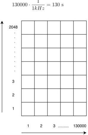
The datasets used for pulse compression and Doppler processing experiments were the NetRAD data sets collected in the United Kingdom and South Africa. NetRAD data sets are stored in binary files as sequential non-delimited 16 bit numbers. Each 16 bit number corresponds to a real valued sample, captured by the analogue-to-digital converter (ADC). Figure 2.2 indicates that received echoes were sampled such that a single range line contains 2048 range bins with an ADC sample rate of 100 MHz [8]. Therefore, the time to sample each range line was:

2048· 1

100 MHz = 20.48 µs (2.2) During the experiments, a total of 130000 pulses were transmitted at a PRF of 1 kHz [8]. This resulted in the experiment lasting for:

130000· 1

1kHz = 130 s (2.3)

Figure 2.2: NetRAD dataset structure

2.2.2

Matched filter

The received signal, x[n], is embedded in additive white noise. A matched filter is a filter that maximizes the signal to noise ratio (SNR) of its output. This is achieved by identifying a known transmitted signal, r[n], within this noisy received waveform. To maximize output SNR, the filter’s transfer function must be a time-reversed and conjugated reference signal [9].

h[n] =r∗[−n] ⇐⇒ H[k] =R∗[k] (2.4) Matched filtering is normally implemented digitally by using fast convolution. Fast con-volution is a correlation operation implemented using the FFT, thus the discrete time samples can be efficiently transformed into discrete-time Fourier transform samples [4]. The fast convolution technique is illustrated in Figure 2.3.

FFT FFT Conjugation IFFT x[n] r[n] X[k] R[k] Y[k] H[k] y[n]

Figure 2.3: An overview of matched filtering in the frequency domain using fast con-volution, taken from NextLook a lightweight, real-time quick look processor for NeX-tRAD [2]

2.2.3

Pulse compression

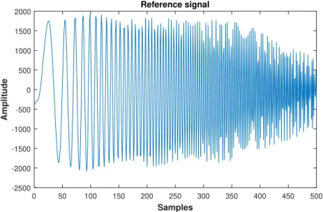
Pulse compression is a modified version of the matched filter whereby the transmitted waveform is modulated. The modulation technique used is linear frequency modulation. This technique produces chirp waveforms, which is a popular choice for radar applications as it is simple to implement and insensitive to Doppler [8]. The chirp pulse used during the experiment has a pulse width of 5 µs, with the number of samples determined by the multiplication of the pulse width and sample rate, therefore giving 500 samples [8]. The chirp pulse is illustrated in Figure 2.4.

Samples 0 50 100 150 200 250 300 350 400 450 500 Amplitude -2500 -2000 -1500 -1000 -500 0 500 1000 1500 2000 Reference signal Powered by TCPDF (www.tcpdf.org) Powered by TCPDF (www.tcpdf.org)

Figure 2.4: Reference chirp used for transmission during NetRAD trial

In order to generate a pulse compressed dataset, the matched filter procedure is applied on the fast time/range dimension of the dataset, implying that the FFT of the LFM chirp is multiplied with the FFT of each pulse of the NetRAD dataset, as shown in Figure 2.5.

Analytic signals

When implementing pulse compression, the Fourier transform of a real valued time do-main signal was taken. It results in a symmetric frequency spectrum, X(−f) = X∗(f). The spectrum, therefore, contains double the amount of information required to recon-struct the original time domain signal. To remove the redundancy, the real signal is extended to an analytic signal, in other words, having no negative frequency components [8]. It is defined mathematically as follows:

Z(f) =          2X(f), f > 0 X(0), f = 0 0, f < 0

Real signals can be extended to analytic signals in the time domain or frequency domain. In the time domain, a process known as Hilbert transform is used. In the frequency domain, the negative spectral components are removed as described above. The real data stored in NetRAD datasets need to be extended to its analytic form before Doppler processing can occur [8].

2.2.4

Doppler processing

By generating a pulse compressed dataset, the output SNR has increased significantly. It is then customary to apply Doppler processing after pulse compression [6]. Pulse Doppler processing is a technique, whereby the energy of a moving target is separated from clutter, implying that the energy of the target would only compete with noise in the targets Doppler bin [4].

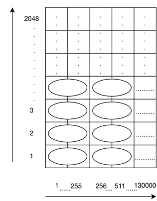
When applying pulse Doppler processing, each range bin is considered, whereby a DFT on each slow time row of the data is computed using an FFT algorithm of a particular size. The size of the FFT corresponds to the coherent processing interval (CPI) [4]. The procedure is depicted in Figure 2.6.

... ... ... ... 130000 1 255 _256....

Slow time/Pulse number

Fast time/Range bins

2048 2 3 1 . . . . . . . . . . . . . . . . . . . . . . . . . . . . . . . . . . . . . . . . . . . . . . . . . . ... 511... Powered by TCPDF (www.tcpdf.org) Powered by TCPDF (www.tcpdf.org)

Figure 2.6: Applying Doppler processing on a pulse compressed data set, where an oval represents a CPI

The DFT bins or CPI corresponds to Doppler frequencies in the range of -P RF₂ to P RF₂ . When deciding on an FFT size, a trade-off exists between spectrum resolution and com-putation overhead. A longer CPI generates more data points, which improves spectrum resolution. However, this requires more memory, as FFTs are longer. Also if the CPI is too long, the target migrates to another range bin. Once the computation is completed, it results in a range/Doppler data matrix, with the dimensions being fast time and Doppler frequency [4, 8].

The importance of pulse Doppler processing, the Doppler shift of a target, can be es-timated by the Doppler bin in which the target was detected. Furthermore, multiple targets can also be detected based on the detections in multiple Doppler bins, provided they are separated enough in Doppler to be resolved [4].

2.2.5

Adaptive noise cancellation

The main objective of the adaptive noise cancellation is to use an adaptive filter to reduce the thermal noise in the received radar signals, such that the weak radar signals can be detected. By using the adaptive filter, thermal noise can be suppressed, with no prior

knowledge of the signal or interference characteristics needed [6]. It is a type of filter that is self adjusting, meaning that the filter parameters are able to change automatically with time [1]. The adaptive noise cancellation technique used was the adaptive line enhancement method, with the least mean squares (LMS) adaptive filter chosen. This adaptive noise cancellation technique can be modelled by Figure 2.7.

delay Adaptive filter

Adaptive algorithm + x[k] = s[k]+n[k] d[k] e[k] y[k]

-Figure 2.7: Block diagram of an adaptive LMS filter taken from [3]

The signal, x[k], is the received signal, which consists of the radar signal of interest, s[n], and broadband noise, n[k]. This received signal, x[k], constructs both the desired signal, d[k], which is equal to x[k] and the input signal to the adaptive filter, which is a delayed version of x[k]. The delay, ∆, must be chosen such that the broadband noise in the desired and delayed signals becomes uncorrelated but still has the radar signal correlated. The adaptive filter attempts to minimize the error signal such that the correlated periodic components are passed and broadband noise is rejected. The output signal, y[k], of the adaptive filter will attempt to create the radar signal of interest, s[k] [3].

The adaptive filter coefficients for a finite impulse response filter are represented at each time step, k, by a vector, wk, of length, L.

wk= [w0 w1 ... wL]T (2.5)

The input into the adaptive LMS filter is a delayed version of x[k]. It can be represented at each time step, k, as follows:

The radar signal of interest, s[k], is embedded in noise. The output of the adaptive filter, y[k], attempts to create this radar signal of interest and is denoted by Equation (2.7):

y[k] =w_kT ·xk (2.7)

At each time step, the adaptive filter coefficients, wk, are updated by an adaptive

algo-rithm. The adaptive filter algorithm consists of a mean square error (MSE) objective function. The MSE is a function of the error signal, e[k].

e[k] =d[k]−y[k] (2.8) Since y[n] goes towards the signal of interest, s[n], the error signal will be approximate thermal noise.

e[k] =d[k]−y[k] =s[n] +n[n]−s[n]≈n[n] (2.9) To minimize the MSE, the adaptive filter coefficients are altered recursively as follows:

wk+1 =wk+ 2µ·e∗(k)·xk (2.10)

where ∗ represents complex conjugate.

The step size, µ, is also known as the convergence factor. This determines the change of the filter coefficients in each time step. By using a small step size, changes to the filter parameters are small in each time step. This results in a high convergence time, as steps towards the minimum of the performance surface are short. The advantage is that, the steady state MSE will be small. However, a large step size is the opposite, as it gives a fast convergence time and an increase in steady state MSE. Therefore, choosing an appropriate step size becomes a tradeoff between having a fast convergence time or a small steady state MSE [10].

The other important parameter needed for the LMS filter is the filter length. This determines the best SNR performance that the adaptive filter can achieve. A small number of filter coefficients will give a low SNR gain, while a large number of filter

coefficients generate a high SNR gain. Having many filter coefficients requires more samples, resulting in a longer time to converge [10].

2.3

Programming languages

Users design algorithms in high-level languages, consisting of basic English words and phrases, arithmetic operators and punctuation. A program written in a high level lan-guage is known as source code. Computers will not be able to execute source code; therefore it needs to be converted to machine code. Machine code is written in binary, 0’s and 1’s, which is understandable by a computer. In order to convert source code to machine code, either compilers or interpreters are used [11].

Compiled programming languages: These are programming languages that goes

through a compiling step during which all of the source code is converted to machine code. The machine code generated is then executed directly on the target hardware. In other words, during runtime, only machine code is executed. Compiled languages also optimize generated code to achieve faster execution [12].

Interpreted programming languages: When using interpreted languages, source code

is not converted to machine code prior to runtime. There is no explicit compile step. During runtime, interpreted languages are executed one command at a time by another program, known as an interpreter program. It therefore interprets the source code and then executes previously compiled functions based on that source code during runtime and not before runtime as for compiled languages. For this very reason interpreted languages can be considered slower than compiled languages [12].

All of the investigated packages contain interpreted languages and RSP algorithms are developed on a Linux system. The open source packages are all available from the Linux distribution packaging system. However, the up-to-date versions might not be available, therefore, for certain languages, the binary version of the packages was used. A binary version of a software package is a pre-compiled version that can be read by the computer and used for execution.

2.3.1

MATLAB

MATLAB stands for MATrix LABoratory. It is a high performance language, used for technical computing, and has been commercially available since 1984 [13]. It has grown to be considered as a standard tool used by most universities and industries. There are numerous powerful built-in science and engineering toolboxes available, used for a variety of computations. These comprise signal processing, control theory, symbolic computation and many more [13]. MATLAB 2014 was the licenced version used for RSP designs. To get a MATLAB licence is expensive, which is why free, open source alternatives need to be considered.

2.3.2

Julia

Julia is a high-level language that achieves high performance for numerical computing. It also provides a just-in-time (JIT) compiler, numerical accuracy and a comprehensive mathematical function library. Julia’s base library is mostly written in Julia, integrating C and FORTRAN libraries for linear algebra and signal processing. Currently, the Julia developer community is rapidly contributing numerous external packages through Julia’s built-in package. Julia 0.5.2, which was updated in May 2017, was used in the develop-ment of RSP algorithms. A new, much improved version, Julia 0.6.0, is available but still in its infant stage, with algorithms on Julia 0.5.2 completed before Julia 0.6 was released [14].

2.3.3

Scilab

Scilab is a free, open source software package provided under the Cecill licence. It is used for numerical computations, as it provides a powerful computing environment for engineering and scientific applications. It includes various functionalities such as signal processing, control system design and analysis, and many more [15]. On the Linux system used for the experiments, the packaging system is distributed with Scilab. The up-to-date version, Scilab 6.0.0, was, however, not available on that particular Linux version, therefore the binary version of Scilab 6.0.0 was used. Reasons for using Scilab 6.0.0 were that memory was dynamically allocated and previous versions of Scilab only accept approximately 2GB of memory. This was not sufficient when large datasets need to be processed. Algorithms were also implemented on Linux systems because the Windows

version of Scilab 6.0.0 immediately shuts down for unknown reasons when processing the datasets. This happened on multiple Windows systems. The latest version of Scilab 6.0.0 was downloaded and installed in June 2017.

2.3.4

Octave

Octave was initially developed in 1988 as a companion software, for an undergraduate-level textbook on chemical reactor design. It was later decided to build a more flexible tool which, that was more than just courseware package. Today it is a high level language, intended for numerical computations. Octave is convenient as its syntax is compatible with MATLAB, which is commonly used in industry and academia. Today it is used by thousands of people for numerous activities that include teaching, research and commer-cial applications. It is currently being developed under the leadership of Dr J.W. Eaton and released under the GNU General Public Licence [16]. In the designing of the RSP algorithms Octave 4.0.0 was used as it was initially installed from the Linux distribu-tion package. There are no substantial changes from Octave 4.0.0 to the latest Octave package.

2.3.5

Python

Guido van Rossum invented Python around 1990 while working with the Amoeba dis-tributed operating system and the ABC language. Initially, Python was created as an advanced scripting language for the Amoeba system. Later it was realized that Python’s design was very general, such that it could be used in numerous domains. Today it is a general purpose open source language used for numerous applications [17]. The im-plementation of Python used is the default version, CPython. It is both a compiler and interpreter that comes with standard packages and modules written in standard C [18].

Two versions of Python are currently being used, Python2 and Python3. Python2 is mostly used, it is stable, with no changes being made to it as its life cycle will end approximately in 2020 [19]. Python3 is an improvement on Python2 and will be the future of Python. At the moment it is still growing and updated regularly. The motivation for Python3 was to fix old design mistakes, requiring backward compatibility to be broken from Python2. There would be a few changes in both languages and its libraries, as major Python packages were ported to Python3. This implies that many skills gained by learning Python2 can be transferred to Python3 [20]. The versions of Python used during

this investigation are Python 2.7.12 and Python 3.5.2, which are the default installations on UbuntuMATE 17.04.

Python also has many specialized modules that can be used for solving numerical prob-lems with fast array operations. The Numeric Python (NumPy) package was used in this investigation, as it is an open source numeric programming extension module for Python that consists of a flexible multidimensional array for fast and concise mathematical cal-culations. The internals of this array is based on C arrays, which will give performance improvements, as well as the ability to interface with the existing C and FORTRAN routines. NumPy provides a large library of fast precompiled functions for mathematical and numerical routines that effectively turn Python into a scientific programming tool, allowing for efficient computations on multi-dimensional arrays and matrices [17, 21, 22]. NumPy’s speed is achieved through vectorization, which will be elaborated on in further sections [23].

2.3.6

Additional features for interpreted languages

JIT compiler

When using interpreted languages, faster code can be generated by using a JIT compiler. A JIT compiler uses both the interpreter and compiler, whereby each line is compiled and executed to generate machine code. By doing this, the application can be optimized for target hardware [12].

MATLAB and Julia have introduced a JIT, one of the most important factors in how code is executed faster. Currently, Octave’s JIT compiler is in its experimental stage, while CPython and Scilab do not have such a feature. However, Python makes use of the CPython compiler, which is not optimized for numerical processing. This compiler could be replaced with the Numba compiler that would give CPython JIT capabilities but it is not compatible with all the existing Python libraries (mainly Pyfftw) and some of the language features [24]. Another Python implementation known as PyPy imple-ments a standard JIT compiler, this also has the libraries issues that Numba does [25]. The disadvantage of languages with a JIT compiler is that the first run is always slower than subsequent runs because of the compilation process. Therefore, when performing benchmarks, always use the second runs [12]. A JIT compiler also performs optimiza-tion techniques, such as vectorizaoptimiza-tion on for loops in the background, resulting in loop overhead being minimized. MATLAB’s JIT compiler has been improved significantly in

newer versions, speeding upfor loops without the user’s attempt to vectorize them [26].

Python JIT compiler

Implicit parallelism

There are several forms of parallelism that can be implemented in algorithms. These can be classified into either implicit or explicit parallelization. The former is where the user’s code is parallelized without any modification to the algorithm, while the latter is a transformation of the user’s algorithm to achieve parallelization [27, 28]. During this investigation, implicit parallelization was constantly used, as it occurs without the users knowledge. There are two types of implicit parallelism: vectorization and linear algebra computations.

Vectorization: This is a programming technique whereby vector operations are used,

instead of element-by-element loop-based operations. Vectorized operations are implic-itly parallelized. This means that the internal implementations are optimized by being multi threaded behind the scenes in optimized, pre-compiled C code. When possible, it also makes use of the hardware’s vector instructions or performs other optimizations in software that accelerates everything. A JIT compiler is important as one of its features is vectorizing for loops in the background, such that loop overhead is minimized. The three main advantages of vectorized code are [29, 30]:

1. Appearance of the code is neater, which is easier to understand.

2. It is faster than loop based code, as its operations are optimized for matrices and vectors.

3. It is typically shorter than loop-based code, which is less prone to errors.

In most scenarios vectorized code achieves a massive speed up compared to loop based code [31]. All of the above languages have operations which are optimized for matrices and vectors.

Linear algebra computations: Implicit parallelization also shows up in linear algebra

computations, such as matrix multiplication, linear algebra and performing the same operation on a set of numbers [28, 32]. The building blocks for linear algebra is the basic

linear algebra subprograms (BLAS) and Linear Algebra PACKage (LAPACK) libraries [33].

• LAPACK: This is the library responsible for linear algebra computations. It

con-sists of a collection of FORTRAN routines, used for solving high level linear algebra problems [33]. All of the above packages make use of this library.

• BLAS: It is a collection of FORTRAN routines that provide low level operations such as vector addition, dot products and matrix-matrix multiplications [33]. LA-PACK relies on this library for its internal computations [34].

There are four major implementations of the BLAS libraries that can be used. These are reference basic linear algebra subprograms (RefBLAS), automatically tuned linear algebra software (ATLAS), open source basic linear algebra subprograms (OpenBLAS) and intel math kernel library (MKL).

• ATLAS: It provides optimized routines for BLAS, as well as a small subset of

LAPACK. The procedure is based on empirical techniques to provide portable per-formance and improvements over the reference BLAS/LAPACK libraries [33].

• Intel MKL: This is a library developed by Intel. It consists of highly optimized,

heavily threaded math routines for Intel processors. This implies that on Intel processors, maximum performance would be achieved [34, 33]. For computers with Intel CPU’s, these MKL libraries can be obtained for free. If installed correctly, all of the language packages investigated can make use of it for complex matrix operations [35, 36, 37, 38].

• OpenBLAS: For several processor architectures, optimized implementations of

linear algebra kernels are provided [39].

• RefBLAS: Reference BLAS library is a single threaded implementation of BLAS.

For particularly complex linear algebra, this library will be slower than optimized multi-threaded versions [34].

The key difference between these libraries is that RefBLAS is a single threaded implemen-tation and the others are highly optimized, multi-threaded versions of BLAS [34]. Intel MKL is a proprietary library, while RefBLAS, ATLAS and OpenBLAS are open source libraries, all available from the Ubuntu Linux distribution package system [34]. The bi-nary packages of ATLAS and OpenBLAS distributed by Debian are generic packages

which are not optimized for a particular machine [39]. To achieve optimal performance, ATLAS and OpenBLAS must be recompiled locally for optimal performance, which is recommended for advanced Linux users seeking maximum performance. If the hardware used is amd64 or x86, there is no need to recompile OpenBLAS, as the binary includes optimized kernels for several CPU micro-architectures [39].

The default version of BLAS and LAPACK libraries was used for each of the packages and is outlined in Table 2.1. Note that Octave uses OpenBLAS from Linux distribution package by default.

Table 2.1: Default BLAS libraries used for different packages Software BLAS library

MATLAB Intel MKL Julia OpenBLAS Octave OpenBLAS Scilab RefBLAS Python2 OpenBLAS Python3 OpenBLAS

There is a necessity to also have a fair performance comparison. This means that for Scilab, the OpenBLAS library from the Linux distribution package, as well as the default version were considered during the experiment. This was encouraged in order to have multi-threaded BLAS/LAPACK libraries for all software packages, not necessarily being optimized for specific hardware. Note that on Windows, Scilab uses Intel MKL linear algebra libraries by default, instead of the reference linear algebra libraries as with Linux machines.

2.3.7

Memory principles

Memory heap

In any programming language, heap memory management is important. The heap is a massive space where memory is dynamically allocated. In other words, when a program is in execution, it will continuously allocate memory to the heap until algorithms are completed. If the space used on the heap is not freed, that space will never be available again while the program continues to execute. Normally, two scenarios might happen

when this occurs. Firstly, the heap will fill up and the program will abnormally terminate. Secondly, the program would continue to run, but the performance of the system will deteriorate [40].

There are two ways to free space on the heap: manually, whereby programmers must remember to free space that was allocated on the heap or it can be done automatically. Many interpreted languages do the latter. This is accomplished by using a garbage collector which runs as part of the interpreter and checks for space that can be freed on the heap. Garbage collectors will ensure that space on the heap is allocated and accessed correctly. This allows for programmers to allocate space on the heap, without concerning themselves about freeing that space [40].

Virtual memory

Processing datasets that require a significant amount of memory might cause the process-ing procedure to fail or performance might deteriorate, as explained in the memory heap section. To compensate for this, computer systems automatically use virtual memory without the user’s control. Virtual memory is a technique whereby the hardware uses a portion of the hard disk, called a swap file, that extends the amount of available mem-ory. This is completed by treating main memory as cache for most recently used data, the inactive RAM contents are stored onto disk and only active contents are allowed to be situated in main memory. This process is continued as needed by the computer by continuously swapping from disk to memory, eventually causing the system performance to deteriorate [41].

Principle of locality

Over the years, memory performance has not increased at the same rate as CPU perfor-mance. When processing large datasets, generating fast algorithms could be troublesome, as performance will be limited by the time it takes to access memory. Code is thus mem-ory bound, which means that processing is decided by the amount of memmem-ory required to hold the datasets. However, there are measures that can overcome memory bound code, such as avoiding inefficient memory usages [42].

Principal of locality is an important concept for cache friendly code, which is when the same or related storage locations are being accessed regularly [43, 4]. It allocates data

such that it is aligned close in memory. There are two types:

Temporal locality: When data in a specific memory location is accessed and cached

-data that is accessed can be used again for a short time period.

Spatial locality: Relevant when manipulating datasets, the data in a particular dataset

are aligned in memory locations that are close to each other. When accessing elements in matrices, elements adjacent/next to it will also be fetched.

When the user generates code to manipulate data, both forms of locality are likely to occur. By considering spatial locality, datasets can be manipulated to ensure that it handles contiguous memory effectively. This will lead to fewer memory accesses and faster code [43].

Contiguous memory

When processing 2-D or an N-D array, try accessing data that transverses monotonically increasing memory locations [42]. This means either accessing rows or columns, depending on how data is stored in contiguous memory. When accessing memory, data is not directly read from it, some of the data is initially stored from memory to cache, and then read from cache to the processor. If data needed is not in cache, the required data will be fetched from memory. This process can be referred to as spatial locality: when fetching an element, the elements next to it are cached. To ensure spatial locality occurs for the RSP algorithms, row major or column major ordering needs to be considered [44].

Figure 2.8 demonstrates spatial locality using a simple 3x3 matrix with data for row and column major ordering schemes.

a b c

d e f

g h i

(a) Block diagram of memory block configuration.

a b c

d e f

g h i

(b) Contiguous memory block configuration for row major.

a b c

d e f

g h i

(c) Contiguous memory block configuration for column major.

Figure 2.8: Demonstration of spatial locality of a matrix of data.

Figure 2.8(b) demonstrates row major ordering, whereby the data will be processed from left to right. The value at position a is read from memory and values at positions b and c will be cached. This implies that the first row must be processed or accessed first before the next row is accessed or processed. Column major ordering is the reversed procedure, as shown in 2.8(c), with one column being processed before the next column. Considering this ordering scheme before applying operations results in fewer memory accesses and more cache accesses. This would lead to faster code, as modern CPUs make use of a faster cache, reducing the average time taken to access main memory. This results in maximum cache efficiency when large datasets need to be processed [42]. Python uses row major ordering by default, while all of the other packages use column major ordering.

2.3.8

FFT library

When pulse compression and Doppler processing are applied to a particular dataset, the FFT operation is required. Implementing fast FFTs is beneficial if the datasets are large. The library used to achieve fast FFTs is FFTW, the "Fastest Fourier Transform in the West". It is a free portable C package developed by MIT. FFTW is based on the

Cooley-Tukey fast Fourier transform, that takes real data and computes the complex discrete Fourier transforms (DFT) inN log(N) time. This library is considered to be much faster than available DFT software, as well as being on par with proprietary, highly tuned libraries [8, 45].

The user also has the ability to interact with the FFTW library through the planner method which helps the FFTW to adapt its algorithm to the hardware of the ma-chine. FFTW is thus optimized by the planner during runtime. FFTW’s performance is portable, as the same code can be used to achieve good performance on various hardware types. Different types of planner methods can be used. The user can decide on a planner that runs all tests, including ones that are not optimal, to determine the best transform algorithm for the dataset. This type of planner would result in a higher computational cost, however the least computational cost algorithm would be used for the experiments in this investigation [8]. The planner that can accomplish this scenario is the estimate planner, which will give the best guess transform algorithm based on the size of the problem [46].

When using the FFTW, the number of operations is proposed to be 2.5N log(N) and 5N log(N) [47]. This is for the real and complex transforms respectively, where N is the number of values to be transformed. It is not an actual flop count, but a convenient scaling based on the radix-2 Cooley-Tukey algorithm and it is based on Big O notation. Big O notation describes the performance or complexity of an algorithm, giving information about the rate of growth of an algorithm as the size of the input increases [48]. This means that as N increases, the runtime will be proportional to 2.5N log(N) and 5N log(N) for real and complex transforms respectively [47, 48]. The proposed values are viable for this investigation, because it was used in many scenarios to generate benchmark tests for performance analysis [49]. All of the languages use FFTW by default apart from Python which requires the Pyfftw library. The procedure for Pyfftw is mentioned in the Appendix section.

2.3.9

Floating point operations per second (FLOPS)

A floating point number is one where the position of the decimal point can float rather than being in a fixed position within a number [50]. When mathematical operations are applied on floating point numbers, these operations are called floating point operations. In scientific computing, a common procedure is to count the number of floating point operations carried out by an algorithm [51]. The floating point operations used in this

investigation include multiplication, division, addition, subtraction and the FFT function. Some of the above operations are applied on complex values. To estimate the central processing unit (CPU) or hardware performance, it is necessary to convert complex valued operations to real valued operations. Table 2.2 illustrates a list of how many real valued operations were used for each operation.

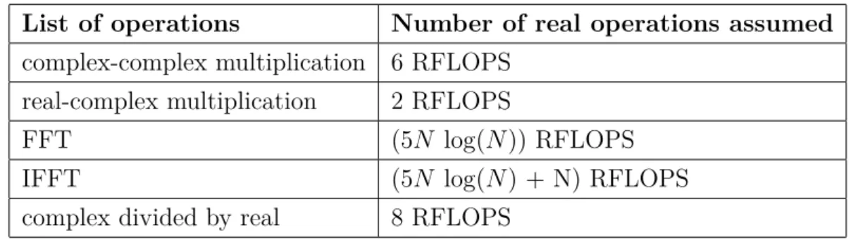
Table 2.2: Basic number of operations used in RSP algorithms

List of operations Number of real operations assumed

complex-complex multiplication 6 RFLOPS real-complex multiplication 2 RFLOPS

FFT (5N log(N)) RFLOPS

IFFT (5N log(N) + N) RFLOPS

complex divided by real 8 RFLOPS

The values for the operations in Table 2.2 are taken from [47, 52]. The complex divided by real was determined by 1 real inverse + 1 real-complex multiply. A real inverse is assumed to be 6 RFLOPS because the number of operations for it varies significantly on different hardware and a real-complex multiplication is 2 RFLOPS [52]. This then gives a total of 8 RFLOPS for a complex divided by a real.

To get an estimate of how fast the CPU can process the floating point operations (FLOPs) of an algorithm on different language packages, FLOPS need to be determined [53]. This can be defined by the FLOPs for the floating point operation used, divided by how long it takes to compute that specific operation.

F LOP S = F LOP s

Implementation of radar signal

processing (RSP) techniques

3.1

Fairness

In the design process of the algorithms, four main considerations were taken into account to ensure a fair algorithmic comparison across the different languages.

• Float64 numbers: This is to achieve maximum accuracy and precision when

computations take place. Double precision numbers also occupy more memory than Float32 numbers, indicating how well the software packages handle algorithms that use maximum computer resources. This could be considered as a worst case scenario in terms of computer resource usage.

• Spatial locality: This ensures that the contiguous memory block is used effectively

for each of the language packages. It makes sure that one language is not given an advantage over another language - all software packages will have the same amount of memory accesses and the same amount of data will be cached.

• Same libraries: The only library used was the FFTW library and all of the

lan-guages made use of the estimate planner. No additional libraries were used during the actual design of the algorithms, with the exception of Python. For Python, the NumPy library is encouraged because it gives Python scripting language capabili-ties such as vectorization. During the actual experiment to get speed results, the file I/O, graphics was ignored as it is not part of the actual signal processing of the

algorithms.

• Similar implementation: All of the RSP algorithms across all of the software

packages will have the same algorithmic implementation.

3.2

Pulse compression implementation

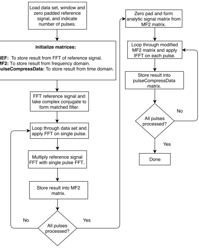
The pulse compression algorithm is basically the matched filter implementation described in the previous chapter. Figure 3.1 illustrates the procedure followed to implement the pulse compression on the NetRAD dataset.

1. The dataset is read into memory as a two dimensional matrix of size N, where N = number of range bins ×number of pulses. In Python, it is read in the reversed direction (number of pulses×number of range lines). This is because its contiguous memory block is in row major ordering instead of column major ordering.

2. Reference signal or transmitted pulse is read from a text file into a one dimensional matrix. The reference signal was windowed by applying a Hanning window [54]. Since the reference signal has only 500 samples, it was zero padded such that it has 2048 samples. This ensures that it has the same amount of samples as a single pulse in the datamatrix. The reference signal was also transposed.

3. The FFT of the reference signal is multiplied with the FFT of each line of the data-matrix. This is done sequentially in a for loopfor a specific number of pulses stipulated by the user. The output is then stored in the MF2 matrix.

4. Analytic signal is formed by taking the completed MF2 matrix and zeroing the negative half of it. Since the MF2 matrix has 2048 samples, the first 1024 samples were zeroed, leaving only the positive half of the spectrum.

5. Inverse FFT is applied on each pulse of the modified MF2 matrix with the result stored in pulseCompressData matrix.

Load data set, window and zero padded reference

signal, and indicate number of pulses.

Initialize matrices:

REF:  To store result from FFT of reference signal. MF2: To store result from frequency domain. 

pulseCompressData: To store result from time domain.

FFT reference signal and take complex conjugate to

form matched filter.

Loop through data set and apply FFT on single pulse.

All pulses processed? Multiply reference signal FFT with single pulse FFT..

Store result into MF2 matrix.

No

Zero pad and form analytic signal matrix from

MF2 matrix.

Loop through modified MF2 matrix and apply IFFT on each pulse.

All pulses processed? No Done Yes Yes

Store result into pulseCompressData

matrix.

Figure 3.1: Algorithm design for pulse compression

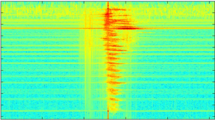
Typically, the pulse compressed data was visualised by a range-time intensity (RTI) plot. This is a two-dimensional image plot, with the x-axis representing slow time, y-axis representing fast time and the amplitude of each pulse as the range of colour. Figure 3.2 represents an RTI plot of a particular NetRAD dataset, as well as the pulse compressed version.

0 20000 40000 60000 80000 100000 120000 Pulse number 0 500 1000 1500 2000 Range bins

Before pulse compression

(a) RTI plot of raw NetRAD radar data.

0 20000 40000 60000 80000 100000 120000 Pulse number 0 500 1000 1500 2000 Range bins

After pulse compression

(b) RTI plot of pulse compressed NetRAD dataset.

Figure 3.2: RTI plot before and after pulse compression

It is important to note that the dataset is a scene of the ocean. In (b) the pulse compressed version of (a) shows high intensity curves. This illustrates that ocean waves are moving towards the radar over time. This also indicates that SNR has improved, as more valuable information can be interpreted from the pulse compressed dataset. To get even more information from this dataset Doppler processing can now be applied.

3.3

Doppler processing implementation

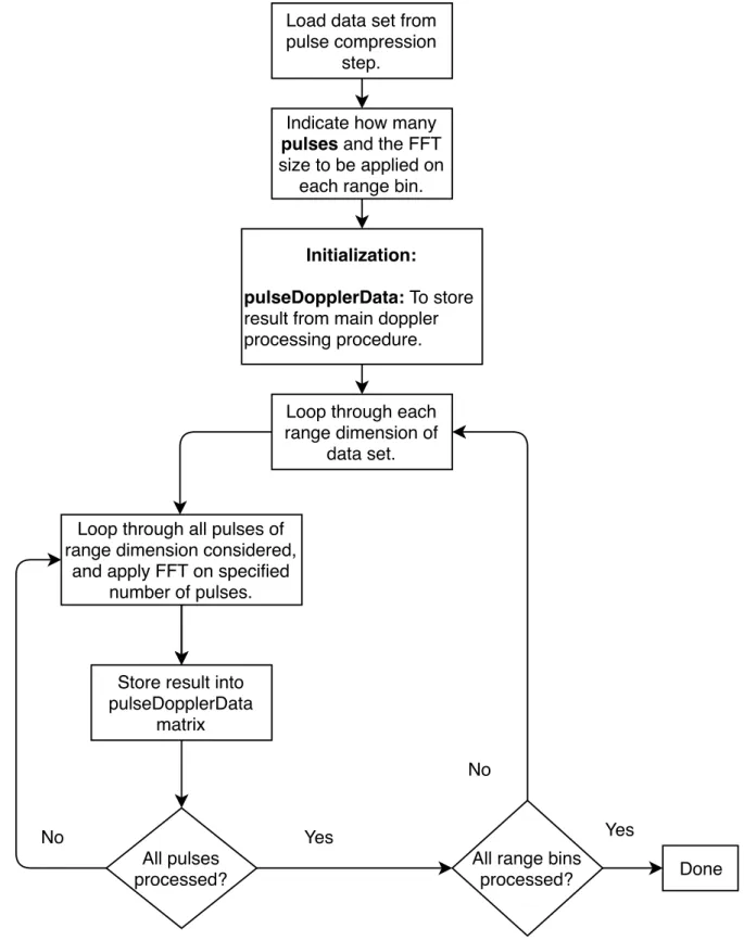
To perform Doppler processing, the output data matrix from the pulse compression was used. Figure 3.3 displays the procedure followed to generate range Doppler matrix.

1. The data matrix from pulse compression algorithm was loaded and then transposed. This gives the data matrix with dimensions of (number of pulses×number of range lines) for column major ordering and (number of range lines×number of pulses) for row major ordering. This allows for the exploitation of contiguous memory storage of each language package. In other words, there will be more cache accesses and fewer memory accesses when the FFT operations are applied.

2. To produce a Doppler spectrum, CPI needs to be defined. This is the FFT size which is applied to all pulses of each range bin. During the experiment, the FFT size was de-termined empirically. An FFT size of 256 was chosen, as it gave a compromise between computation time and spectrum resolution. The result was stored in the pulseDoppler-Data matrix.

Load data set from pulse compression

step.

Indicate how many

pulses and the FFT

size to be applied on each range bin.

Loop through all pulses of range dimension considered,

and apply FFT on specified number of pulses.

All pulses processed?

All range bins processed? Loop through each

range dimension of data set. No Yes No Done Initialization: pulseDopplerData: To store

result from main doppler processing procedure.

Yes Store result into

pulseDopplerData matrix

Figure 3.3: Algorithm design for Doppler processing

Figure 3.4 shows a range Doppler plot for the first 256 pulses, illustrating Doppler shifts of targets for a specific range, over short instance in time.

Range Doppler plot of a NetRAD dataset DFT bins 50 100 150 200 250 Range bins 200 400 600 800 1000 1200 1400 1600 1800 2000

Figure 3.4: Range and amplitude of Doppler frequencies at different range bins

Figure 3.4 shows several targets that were detected at positive Doppler frequencies as Doppler bins from 0 to 256 represent Doppler frequencies from -0.5 kHz to 0.5 kHz.

3.4

Adaptive LMS filter implementation

The adaptive LMS filter is identical to the implementation that was described in the previous chapter. Figure 3.5 shows the procedure that was followed to implement the adaptive LMS filter on a simulated dataset.

1. The noisy dataset is read into memory as a one dimensional array/vector. A one dimensional array/vector is stored in a contiguous block of memory by default.

2. Step size and filter length were chosen, that gave a reasonable convergence rate with a small MSE, and a suitable SNR.

3. The (delay_x) signal is the noisy dataset signal vector that is delayed by five samples to ensure the noise is uncorrelated from it. Five samples was chosen because there are about 2.5 samples per signal period. This shifting of the vector is completed by adding zeros to the beginning of the vector.

4. The filter length of 80 was chosen. This means that 80 samples of the delay_xsignal were stored into vector x.

5. A weight vector of length 80 is multiplied with the x vector, with the result stored into array/vector y.

6. Error vector is calculated by using equation (2.8) , the parameters inserted were the noisy dataset vector from Step 1 and y vector from Step 4.

7. Weight vector is updated from equation (2.10) by using the step size as well as the weight, error and the x vector from the above results.

Load noisy data set into a vector with N amount of samples.  delay_x: Delay dataset vector by n number of samples. Choose step size,m and filter

length,L.

i = N-L? Store (i : i+L-1) samples from the delay_x vector into x

vector

i++

multiply x vector with w vector.

Store result into y vector. Calculate error vector from equation (2.8). Update weight vector from equation (2.10) No Done Yes Initialization w: weight vector,size L. e: error vector, size N-L. y: filtered output vector,N-L.

x: To store input into adaptive filter. n: Choose number of samples to

delay data set signal vector.

The dataset used for LMS filter was radar signals generated in MATLAB. The signal consists of fixed frequency pulses with additive white Gaussian noise. The parameters of this signal are shown in Table 3.1:

Table 3.1: Fixed frequency signal parameters

Signal parameters Value

Frequency 500 MHz

Sampling frequency 1280 MHz

Amplitude 1

Pulse width 2 µs

Pulse repetition interval 20µs

Simulation time 50µs

The signal was then saved to a text file, such that the same simulated radar data was used for all of the language packages. Figure 3.6 illustrates the noisy dataset which was loaded into the LMS algorithm for the experiment, as well as the output of the LMS filter which suppressed the thermal noise.

Number of samples #104 0 1 2 3 4 5 6 Amplitude -5 -4 -3 -2 -1 0 1 2 3

4 Before adaptive LMS filter

(a) Fixed frequency pulse with noise simulated in MATLAB.

Number of samples #104 0 1 2 3 4 5 6 Amplitude -2 -1.5 -1 -0.5 0 0.5 1 1.5

2 After adaptive LMS filter

(b) Output of LMS adaptive filter.

Figure 3.6: Simulated fixed frequency pulse radar signals before and after LMS adap-tive filtering

Results and discussion

In this chapter, the performance related results will be shown for three RSP algorithms. These are pulse compression, Doppler processing and LMS filter. In order to evaluate the performance of pulse compression and Doppler processing on all packages, three different experiments were undertaken:

1.) Computation time: Determines the wall clock time for the RSP algorithms in

various language packages. Wall clock time is the actual time taken, from the start of the RSP algorithms to the end. This determines which software package would complete the quickest.

2.) Memory handling: Gives an indication of how memory is used for all of the language

packages, by considering if the calculated memory or extra memory was used during processing. This was completed only for pulse compression and Doppler processing, as the NetRAD datasets required a lot of memory. It was not worthwhile completing this for small sets of data that was used for the adaptive LMS filter.

3.) FLOPS: This gives an indication of how many mathematical operations are

per-formed for different RSP algorithms on various language packages.

By evaluating the performance of the experiments and comparing it with all the lan-guage packages under investigation, the objectives of the study can be met. Note: thesis algorithms can be found on bitbucket (https://bitbucket.org/ExtremesExtreme/thesis-code/src/master/)

4.1

Performance of RSP algorithm designs

The standard parameters used for computing pulse compression and Doppler processing from the NetRAD dataset are as follows:

Table 4.1: Standard specifications used during pulse compression and Doppler pro-cessing

Range lines Range bins Doppler bins

130000 2048 256

In order to evaluate computation time, the number of range lines was altered. All of the RSP techniques were benchmarked with the following fairness simulation criteria:

• No loading of binary and text files into memory was considered during the perfor-mance analysis.

• No GUI interface was considered while the RSP algorithms on each of the language packages were executed.

• Programs ran under the same conditions, no other users were using the server com-puter and no other programs but the RSP algorithms were executing. This ensures maximum performance and fair comparison for each of the language packages.

The hardware used for the software packages performance analysis was the following:

Table 4.2: Hardware specification used for the computation of the RSP techniques Hardware specifications

CPU Intel(R) Core(TM) i7 960 CPU clock(GHz) 3.2 GHz

RAM 25.77 GB

4.1.1

Computation time for pulse compression design

Commonly the number of range lines is altered to measure the performance of pulse compression. It gives an indication of how well the algorithms handle larger sets of data.

Figure 4.1 and 4.2 illustrates the performance of pulse compression as the number of range lines was varied from 13000 to 130000.

Number of pulses _#104 2 4 6 8 10 12 Execution time(s) 0 10 20 30 40 50 60

Execution time vs number of pulses for pulse compression

Julia MATLAB Octave Scilab Python2 Python3 Powered by TCPDF (www.tcpdf.org) Powered by TCPDF (www.tcpdf.org) Powered by TCPDF (www.tcpdf.org)

Figure 4.1: Time taken for pulse compression

Number of pulses #104 2 4 6 8 10 12 Execution time(s) 0 10 20 30 40 50 60 70 80

Execution time for pulse compression for non contiguous memory accessess

Julia MATLAB Octave Scilab Python2 Powered by TCPDF (www.tcpdf.org) Powered by TCPDF (www.tcpdf.org)

Figure 4.2: Time taken for pulse compression with different indices

Figure 4.1 illustrates a nearly linear relationship between the number of pulses and com-putation time. The trend was expected, as more data is processed the longer the program takes to execute. The most important observation: the same algorithm ran on numerous language packages but the computation times varied. MATLAB, Julia and Python all had similar results, varying from 9 to 12 seconds, with Python being the fastest. Octave and Scilab were the slowest at 28 and 63 seconds respectively. Figure 4.1 trends are much faster than Figure 4.2, because it is cache friendlier, as it does not have non-contiguous memory accesses.

There is no JIT compiler built into Octave and Scilab, but CPython, the default Python version, has a compiler which is not optimized for numerical processing. Since processing is completed in afor loop, the loop will not be vectorized automatically, Python’s NumPy and Pyfftw libraries are however highly optimized for numerical computations applied on NumPy arrays, resulting in faster execution time. In order to see if vectorization was the problem, specifically for Octave and Scilab, vectorization techniques were applied when possible in all of the language packages. This means that instead of using a for loop, a vector was used to index the data matrix to apply processing. In some scenarios, processing could not be completed without a loop, therefore it could be interpreted that loops were minimized as much as possible in the design. Figure 4.3 illustrates the result after vectorization was applied to the pulse compression algorithm for each of the language packages. Number of pulses _#104 2 4 6 8 10 12 Execution time(s) 0 5 10 15 20 25 30 35 40 45 50

Execution time vs number of pulses for pulse compression Julia MATLAB Octave Scilab Python2 Python3 Powered by TCPDF (www.tcpdf.org) Powered by TCPDF (www.tcpdf.org)

Figure 4.3: Vectorization implementation for pulse compression

Figure 4.3 emphasizes that there was an improvement in MATLAB, Octave and Scilab. Octave computed processing in approximately 16 seconds, while Scilab was still signifi-cantly slower than the rest of the packages.

Another reason for the discrepancy in Scilab’s computation time could be from implicit parallelization. Scilab employed the reference BLAS library by default, which used one core when doing matrix multiplication. To investigate if this was the problem, a different BLAS library was used, namely OpenBlas library from the Linux distribution package. This library was applied to the loop based and semi-vectorized code, with the results depicted in Figure 4.4

Number of pulses _#104 2 4 6 8 10 12 Execution time(s) 0 10 20 30 40 50 60

Execution time for pulse compression using different BLAS libraries on Scilab Scilab using default BLAS library