Learning with Kernels on Graphs: DAG-based kernels, data streams and RNA function prediction.

(1)

Alma Mater Studiorum - Universit`

a di Bologna

DOTTORATO DI RICERCA IN INFORMATICA

Ciclo: XXVI

Settore Concorsuale di afferenza: 01/B1

Settore Scientifico disciplinare: INF01

Learning with Kernels on Graphs:

DAG-based kernels, data streams and RNA

function prediction.

Presentata da: Nicol`

o Navarin

Coordinatore Dottorato:

Relatore:

Maurizio Gabbrielli

Alessandro Sperduti

(2)

(3)

Abstract

In many application domains such as chemoinformatics, computer vision or natural language processing, data can be naturally represented as graphs. Machine learning allows for computers to learn a concept from a set of examples. When the appli-cation of analytical solutions for a given problem is computationally unfeasible or we do not know how to analytically solve a problem, machine learning techniques could be a viable way to solve the problem. Classical machine learning techniques are defined for data represented in a vectorial form. Recently some of them have been extended to deal directly with structured data. Among those techniques, ker-nel methods have shown promising results both from the computational complexity and the predictive performance point of view. Moreover, these methods offer strong theoretical guarantees on the quality of the solution. Kernel methods allow to avoid an explicit mapping in a vectorial form relying on kernel functions, which informally are functions calculating a similarity measure between two entities. However, the definition of good kernels for graphs is a challenging problem because of the difficulty to find a good tradeoff between computational complexity and expressiveness. An-other problem we face is learning on data streams, where a potentially unbounded sequence of data is generated by some sources. We considered the case where the learning algorithms have to respect a bound on memory occupation.

There are three main contributions in this thesis.

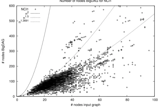
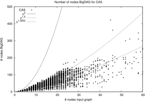
The first contribution is the definition of a new family of kernels for graphs. The idea is to decompose a graph into a multiset of simpler structures, i.e. Directed

(4)

results from both the computational and the classification point of view on real-world datasets.

The second contribution consists in making the application of learning algorithms for streams of graphs feasible. Moreover, when memory constraints are present, the adopted budget management policy is critically influencing the overall algorithm performance. We defined a principled way for the management of the budget, based onLossyCounting, which is an algorithm originally designed for computing approx-imated frequency counts over event streams. Our proposal extends LossyCounting

in order to approximate the solution of a learning algorithm.

The third contribution is the application of machine learning techniques for structured data to a bioinformatics problem, namely non-coding RNA function prediction. In this setting, the secondary structure is thought to carry relevant information. However, existing methods considering the secondary structure have prohibitively high computational complexity, thus limiting their application to very small datasets. Indeed, the tool that is considered the state-of-the-art considers only sequence information. We propose a new representation for RNA sequences. More-over, we adapted the definition of existing graph kernels, and defined a new one, on such representation. The resulting kernels are able to consider the secondary struc-ture and are fast enough to be applied to large datasets. Our proposed approach outperforms the state-of-the-art.

(5)

Acknowledgements

Foremost, I would like to thank my advisor Prof. Alessandro Sperduti for his guid-ance and support. Besides my advisor, I would like to thank Dr. Giovanni Da San Martino who helped me at different stages of my PhD journey.

Next, I thank Dr. Fabrizio Costa for giving me the opportunity to visit the Bioin-formatics group at the University of Freiburg.

Also, I need to thank my PhD colleagues that made this experience more pleasant and unique.

Thanks to all the people that supported me during these difficult years.

Last but not least, I would like to thank my family for allowing me to realize my own potential. My mother gave me the opportunity to follow university and then the doctoral program. My father helped me to get through the tough times.

(6)

(7)

Original Contributions

74

4 A new framework for the definition of DAG-based graph kernels 75 4.1 A new DAG-based kernel framework for graphs . . . 77

4.1.1 Decomposition of a graph into DAGs and derived graph kernels 78 4.2 Extending tree kernels to DAGs . . . 81

4.2.1 Ordering DAG vertices . . . 82 ix

(10)

4.2.4 Speeding up the kernel matrix computation . . . 90

4.2.5 Limiting the depth of the visits . . . 92

4.3 Two graph kernels based on the framework . . . 93

4.3.1 A graph kernel based on the Subtree Kernel . . . 93

4.3.2 A graph kernel based on a novel tree kernel . . . 97

4.3.3 Feature spaces comparison of some graph kernels . . . 98

4.4 Experimental results . . . 100

4.4.1 Dataset Description . . . 102

4.4.2 Results and Discussion . . . 102

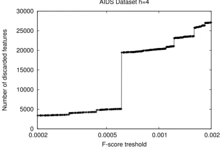
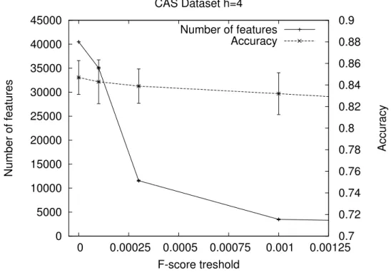
4.5 Model compression . . . 111

4.5.1 Application of feature selection to graph kernels . . . 112

4.5.2 Experimental results . . . 114

5 Learning algorithms for streams of graphs 119 5.1 Budget online Passive-Aggressive on graph data . . . 122

5.1.1 Removal policies . . . 125

Incremental computation of F-score . . . 126

5.1.2 Experimental results . . . 128

Chemical dataset . . . 128

Image dataset . . . 130

Experimental setup . . . 131

Results and discussion . . . 132

5.2 Budget Passive-Aggressive with Lossy Counting . . . 140

5.2.1 Online frequent pattern mining . . . 141

Lossy Counting . . . 141

5.2.2 Online frequent pattern mining with real weights . . . 141 x

(11)

LCB: Lossy Counting with budget for weighted events . . . . 142

5.2.3 LCB-PA on streams of graphs . . . 144

5.2.4 Experiments . . . 146

Experimental Setup . . . 146

Results and discussion . . . 147

6 Application to RNA 153 6.1 Introduction to RNA . . . 154 6.2 Problem statement . . . 155 6.3 Existing methods . . . 156 6.3.1 Sequence-based methods . . . 156 6.3.2 Structure-based methods . . . 157

RNA secondary structure . . . 157

Infernal . . . 159

6.3.3 Kernel methods . . . 160

Stem kernel . . . 160

Marginalized kernel on RNA sequences . . . 162

6.4 Computation of RNA secondary structure . . . 162

6.4.1 Minimum free energy structure . . . 163

6.4.2 RNA shape representation . . . 164

6.4.3 RNA abstract shapes . . . 166

6.5 Novel graph kernels for RNA sequences . . . 168

6.5.1 Multiple instance learning . . . 169

6.5.2 Representation issues . . . 171

6.5.3 Kernels exploiting different abstraction levels. . . 173

Abstract NSPDK . . . 173

Abstract NSDDK . . . 174

6.6 Experiments . . . 176 xi

(12)

7 Conclusions and future work 183

References 187

(13)

Part I

Introduction and basic concepts

(14)

(15)

Chapter 1

Introduction

The first ultraintelligent machine is the last invention that man need ever make.

I. J. Good, 1965

1.1

Why structured data?

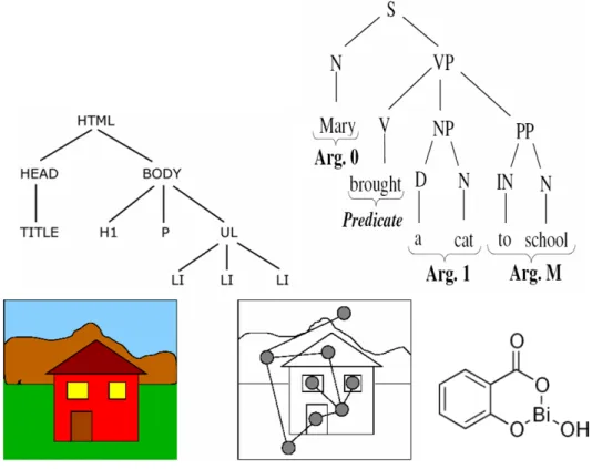
The interest in structured data arises because in many application domains data can be naturally represented in a structured form. For example, XML documents are naturally represented as trees; in NLP each sentence may be represented with its parse tree; in computer vision each image can be represented by its segmenta-tion graph (e.g. [9] or [106]), and in Chemoinformatics chemical compounds can be easily represented as graphs, where each atom is a vertex and the edges represent the bonds between atoms [1]. Figure 1.1 shows some examples of data arising from these applications.

Other application domains where data is naturally represented as graphs include computational biology, social networking, web link analysis or computer networks[1]. The topic of graph data processing is not new. Over the last thirty years there have been continuous efforts in developing new methods for processing graph data. Re-cently, because of the growing amount of structured data and the need to extract

(16)

information from it, there has been the interest, if not the necessity, to apply ma-chine learning on graph data. Nowadays, because of technical advances such as graph kernels [85] and graph mining techniques [153], it is possible to apply these techniques in reasonable time on large datasets, obtaining good results.

Figure 1.1: Examples of data that can be naturally represented in structured form. From left to right, top to bottom: an XML document, a parse tree from NLP, an image and the corresponding segmentation graph and a chemical compound.

1.2

Learning on structured data

The amount of data generated in different areas by computer systems is growing at an extraordinary pace, mainly due to the advent of technologies related to the web, ubiquitous services and embedded systems that aim at monitoring the environment in which they are immersed. According to a report from IDC titled “The Digital

(17)

Chapter 1. Introduction 5

Universe in 2020: Big Data, Bigger Digital Shadows, and Biggest Growth in the far East” [64], only 0.5% of the 643 exabytes of useful data have been analyzed. Examples of this data includes images, social media, sensors (including those in our smartphones and other devices, as well as those that may be implanted into the body), medical devices or biological data, e.g. data generated from DNA sequencers. In this context, to analyze the data means to extract useful information from it. This problem is commonly referred to as Data mining.

For some application domains where huge amounts of data have to be processed, an algorithmic solution may be computationally unfeasible. In other cases, it may be very difficult (or impossible) to state the problem itself in a non-ambiguous way, and thus also the development of an algorithmic solution is very difficult. Finally, it is possible that we know how to formalize the problem but we do not know how to solve it in an algorithmic way. This is the case when looking for the effectiveness of drugs against a certain disease. In these cases, it is convenient to adopt a machine learning approach.

Machine learning [100] is the branch of Artificial Intelligence that lets computers learn from experience. In particular, in our scenario to learn from experience means to learn a concept from examples. A typical learning task is to classify entities. In this scenario, we are given a set of labeled examples and the goal is to learn the concept underpinning the labeling function and to accurately predict the label for unseen examples.

While classical machine learning techniques have been defined for data represented in a vectorial form, more recently many techniques have been extended to deal directly with structured data [141, 46].

In this thesis, we deal with graph classification. There is a second task commonly referred as graph classification consisting in the prediction of the class labels for single nodes in a graph. This latter task is usually faced with different techniques, such as label propagation [29], that are not considered in this thesis.

(18)

1.3

Learning on graph streams

In some application domains, data is generated at a constant rate by sources that can potentially emit an unbounded sequence of data elements, i.e. data streams. Because of that, processing of data streams requires special care from a computa-tional point of view, since only bounded time and memory resources can be used. However, it was early recognized that data streams tend to evolve with time, giving rise to the well-known concept drift phenomenon (see Section2.7.1). Due to compu-tational complexity issues, streams of structured data have not been much studied up to now. Only few works involving streams of trees have recently appeared [5] [72], while not much work has been done for streams of graphs.

This is a major drawback, since in many important application areas data can nat-urally be represented as streams in structured form. For example, modern medicine critically depends on the discovery of new drugs, i.e. chemical compounds. Chemical compounds can be naturally described via their molecular graphs. The discovery of new effective drugs relies on the systematic assessment of many different properties of all possible organic molecules, the so-called chemical space, which is estimated at 1020−10200 structures [137]. Only a very small portion of this space (few millions) constitutes the real chemical space, i.e. compounds that have been synthesized, while recent works have explored the possibility to explicitly enumerate a bit larger portion of this space (e.g. in [59] around 26.4 million compounds are covered). Hav-ing to deal with such numbers, it is clear that exploration of the chemical space can only be performed by adopting a stream-based approach, where the same com-pound can occur at different times associated with different but still related classi-fication/prediction tasks. Another example of application involving a graph stream is malware detection. Malware detection consists in recognizing malicious software executed without user’s awareness. The number of codes to be analyzed can be enormous and the problem is difficult since some malwares are able to modify their own code in order to avoid detection. In [56] the detection of malwares is performed by representing executables codes as graph nodes and control flow instructions and

(19)

API calls as edges. Concept drift can be present since malwares continuously try to exploit more and more sophisticated approaches to deceive the classifier. Also classification of images is a task which may involve streams of graphs. In fact, more and more images are available online. A graph can be built from an image with the aim of representing (spatial) relationships between the objects into the image (see Section5.1.2for an example). The task of finding images that a user likes is then an example of a stream of graphs with concept drift. Finally, in [7] a Fault Diagnosis System for Sensor Networks is proposed. The idea is to apply a cognitive algo-rithm to a stream of graphs representing spatial and temporal relationships among the sensors in order to distinguish between changes in the environment and sensor faults. In this context, concept drift occurs naturally as the environment changes. In the aforementioned paper, a simple thresholding system has been used, but the potential for improvements is large if more sophisticated algorithms are adopted.

Learning on graph streams is an important problem, and as such it will be one of the focuses of this thesis.

1.4

Kernel methods

Different approaches in the application of machine learning to structured data have been explored. The simplest one is to define a mapping from structured data to fixed-size vectors in order to straightforwardly apply classical machine learning al-gorithms [93, 90]. Those vectors need to encapsulate structural information about the graph. There are several ways to implement this mapping, some of them suited for specific applications. In general, the more information we keep in the vectorial representation, the more computationally demanding the mapping is. Other ap-proaches are based on graph mining [115]. Basically those methods apply pattern matching techniques to graph data, with the need to solve the subgraph isomorphism problem that is an NP-complete problem.

With the application of kernel methods to graph data, a new promising ap-proach emerged, that mixed the speed benefits of the former with the classification

(20)

performance of the latter. This approach allows to avoid the explicit mapping in a vectorial form and to define learning algorithms directly on the original struc-tured data. For many tasks, kernel methods shows good results outperforming other methods [22,60, 104, 34, 75, 37,122, 105, 111, 85, 9,15, 35, 82,124,53].

Moreover, kernel methods offer strong theoretical guarantees and a convenient hard separation between the learning algorithm and the kernel function that applies directly to the examples and maps them in an high dimensional Euclidean space. The kernel function is, informally, a function that represents the similarity between two objects.

The key for the successful application of kernel methods to graph data is the definition of kernel functions for graphs. Early works [68, 112] defined kernels for graphs with an acceptable expressiveness, i.e. kernels that represent a “meaningful” similarity measure between graphs. However these kernels were computationally de-manding. More recent works defined efficient kernels, some of them with near-linear time complexity [78, 122], but there is a major drawback concerning these kernels. Indeed, it is difficult to find a good tradeoff between computational complexity and expressiveness because, generally speaking, the faster the kernel is, the lower its generalization performance will be.

Recently, the application of graph kernels is being extended to new domains where representing examples as graphs is not straightforward, but this approach allows to explicitly store the information needed from the task. For example, in bioinformatics and molecular biology a significant research topic is the discrimination and detection of functional RNA sequences. The peculiarity of this problem is that in the sequence there is a lot of hidden information. In particular, it is thought that the specific form of the secondary structure is an important feature for detecting RNA sequences (see Chapter6). Recently proposed kernels for RNA sequences [116] try to extract this information from the sequence and incorporate it in the kernel calculation, but the resulting algorithm is not applicable to big datasets. In this thesis we will propose a novel approach for this problem.

(21)

1.5

Contributions

The contributions of this thesis can be grouped in three branches.

The first contribution is the definition of a new family of kernels for graphs. The idea is to define a new similarity measure based on the subtrees of a graph. We analyze two kernels from this family, achieving state-of-the-art results from both the computational and the classification point of view.

The second contribution consists in the definition of learning algorithms for streams of graphs. Namely, we extend a family of online learning algorithms pro-posed in the literature to structured data. It is worth to notice that the algorithms we present are applicable only in conjunction with kernels that allow for an explicit feature space representation, such as the ones defined in the first contribution.

The third contribution is the application of machine learning techniques for struc-tured data to a specific problem from bioinformatics, namely RNA function predic-tion. The application of machine learning to this field is not straightforward because several problems have to be faced. Eventually, we explored some feasible solutions and obtained successful results outperforming the state-of-the-art.

1.6

Outline

This thesis is organized as follows. Part I provides a comprehensive review of the state-of-the-art in the field. We start introducing kernel methods in Chapter 2. In the same chapter, from Section2.7 we present the state-of-the-art on online learning algorithms. Then in Chapter 3 we start talking about learning on structured data and specifically on graphs, giving a comprehensive review of the state-of-the-art in kernel functions for structured data.

Part II groups the original contributions of this thesis. In Chapter4we propose a novel family of graph kernels and we study extensively two members of this family. Moreover, we thoroughly discuss how to make the computation very efficient, and in Section 4.5 how to apply feature selection techniques to the final learned model.

(22)

Part of the work in this chapter has been published in [43] and [44].

These findings are the basics for another study presented in Chapter 5, where the goal is to develop fast online learning algorithms for streams of graphs. We start with an analysis of different possible formulations, proposing a modification of existing learning algorithms that can deal with the explicit feature space of some kernels. Moreover, in Section 5.2 we introduce a brand-new approach to model reduction based on the LossyCounting approach [95], particularly suited for online learning algorithms. This chapter is based on the work published in [45].

Finally, in Chapter 6 we discuss about a particularly interesting problem in bioinformatics, namely non-coding RNA function prediction, and we propose a novel solution based on kernels for graphs. The work in this chapter is a joint work with Fabrizio Costa.

(23)

Chapter 2

Learning with kernels

It is not the strongest of the species that survives, nor the most intelligent, but the one most responsive to change.

Charles Darwin

2.1

Machine Learning

Learning from experience is one central aspect in what humans call intelligence. Indeed, learning from experience is what enables humans to adapt to various situa-tions, and one of the core aspects of intelligent behavior. Learning from experience is a process that everyone adopts every day, during the extraction of physical laws from experimental data or the use of experience for decision making.

Nowadays we don’t have enough information about how humans learn from expe-rience, so we don’t know how to make a computer learn even nearly as well as people do, but many algorithms have been developed that exhibit useful types of learning in some specific tasks. This science that lets computers learn from experience is called machine learning[136].

There are various applications in which machine learning turns to be the most effective approach. A non-exhaustive list includes speech recognition, handwritten

(24)

character recognition, image recognition (and face recognition). The characteristic shared by these problems is that it is very difficult (or impossible) to state the problem itself in a non-ambiguous way, and thus looking for an algorithmic solution for these problems is very difficult.

Moreover, the amount of data collected day by day exceeds the human capability to extract the information hidden in it, so it becomes more and more important to automate the process of learning from data, even so in problems where it may exist an algorithmic solution, but it is too much computationally expensive. The problem of extracting knowledge from data is called data mining.

More formally we say that a computer program is able to learn if its performance improves with experience.

Definition 2.1. [100] A computer program is said to learn from experience E with respect to some class of tasks T and performance measure P, if its performance at tasks in T, as measured by P, improves with experience E .

A textbook example is a computer program that learns how to play chess, that might improve its performance measured as its ability to win, at the class of tasks in-volving playing chess games, through the experience obtained playing against itself. So in general we have to identify these three features in order to have a well-posed learning problem: the class of tasks, the measure of performance and the source of experience.

Machine learning (ML) [99] aims to design and develop algorithms that allow computers to evolve their behaviors based on empirical data, such as from sensor data or databases.

In general, learning involves acquiring general concepts based on some specific training examples. This is not surprising because humans continuously learn general concepts based on examples: think about the concepts of ”bird“ or ”car”. Each one can be viewed as a boolean function defined over a larger set, e.g. a function defined over all animals whose value is true for birds and false for all other animals. There may be some examples that are border line, for which the membership to a class

(25)

Chapter 2. Learning with kernels 13

is not trivial. This kind of examples will be the most important ones in kernel methods, as we will see later.

This decision function is what machine learning methods try to approximate. We can make a taxonomy of different learning problems depending on the nature of the examples and the type of concept we want to learn. A first distinction is between supervised and unsupervised learning. In the former we have a label associated with each instance, while in the latter we don’t. In this thesis we will focus on the supervised learning scenario, but some of the techniques can be applied as-is to the unsupervised one. For details about unsupervised learning, refer to [100]. In supervised learning, we are given a set of tuples called training set of the form

S = {(xi, yi) :i = 1, . . . , n}, where xi ∈ X is the i-th available instance and yi ∈Y

is the associated label. The tuples (xi, yi) are called the examples.

The examples in S are assumed to be generated according to some unknown probability distribution P. Depending on the domain of Y we can further define various types of classification problems:

• If yi ∈ {±1} we have a binary classification problem.

• If yi ∈ {0, . . . , n} we have a multi-class single-label classification problem.

• If yi ∈ {±1}m we have a binary multi-label classification problem.

• If yi ∈R we have a regression problem, that is the problem of approximating

a real-valued target function.

Binary classification is the better understood and studied task. Since many clas-sification methods have been developed specifically for binary clasclas-sification, multi-class multi-classification often requires the combined use of multiple binary multi-classifiers. In this thesis we deal with both types of classification problems.

The goal of supervised learning is to find the function c : X → Y that best represents the relationship betweenxis and yis. Since the only information we know

about this function are the examples in S, the best we can do is try to approximate this function as tightly as possible. The function we want to learn is called the

(26)

(optimal) hypothesis h, that comes from an hypothesis space H that is fixed a-priori (and it must be fixed in order to perform learning). An hypothesis is often referred to as a model, that is an abstraction that tries to explain the reality (in our case tries to explain the evaluation of the unknown cfunction).

The best from all possible hypothesis h, that we will refer to as h∗, is the one that minimizes the risk:

R(h) =

Z

X ×Y

L(h(x), y)dP(x, y)

where L is a loss function that measures the classification error ofh,X is the space of all possible instances and Y the space of the labels.

It’s not possible to directly use this formulation for the selection of the best h

because the probability distribution P(x, y) is unknown. An alternative approach consists in minimizing the error with respect to the data we have, thus defining the

empirical risk: Re(h) = 1 n X (x,y)∈S L(h(x), y) (2.1)

The techniques that select the best model (according to specific criteria) from the set of all possible models (fromH) are referred to as model selection techniques. In the following we will use the concept of Vapnik-Chervonenkis dimension ( VC-dimension) [139] of an hypothesis space H. The VC-dimension is a measure of the capacity of an hypothesis space H, defined as the cardinality of the largest set of points that H can shatter. To shatter a set of points means that, for all possible assignments of labels to those points, there exists a h ∈ H such that h makes no errors when evaluating that set of data points (that is Re(h) = 0).

It is worth to distinguish between two different supervised machine-learning frameworks. Inbatch learning, we assume that there exists a probability distribution over the examples, and that we have access to a training set drawn i.i.d. from this distribution. A batch learning algorithm uses the training set to generate a single output hypothesis. We expect a batch learning algorithm to generalize, in the sense that its output hypothesis should accurately predict the labels of previously unseen examples, which are sampled from the same distribution.

(27)

On the other hand in the online learning framework, we typically make no sta-tistical assumptions regarding the origin of the data. An online learning algorithm receives a sequence of examples and processes these examples one-by-one. On each online-learning round, the algorithm receives an instance and predicts its label using an internal hypothesis, which is kept in memory. Then, the algorithm receives the correct label corresponding to the instance, and uses the new instance-label pair to update and improve its internal hypothesis. The concept of generalization is much more difficult to define for online learning algorithms with respect to the batch ones [27]. Indeed, as we will see in Section 2.7, in online learning the underlying con-cept may change, meaning that the probability distribution over the examples is continuously changing.

The sequence of internal hypotheses constructed by the online algorithm from round to round is referred as the online hypothesis sequence. Typically, online learn-ing have stronger requirements in terms of computational complexity and memory occupation then the batch framework.

2.2

Kernel methods

In many business and scientific applications the use of machine learning methods helped to speed up and reduce the cost of certain processes.

In these research fields, recently a class of learning algorithms has received much attention because of the solid foundation in learning theory and the empirical results that outperforms any other learning method in many benchmarks as well as real-world applications. These are kernel methods, whose most popular example is the Support Vector Machine [138], that will be explained in detail in Section 2.4.2.

Kernel methods are all the learning algorithms that can represent the solution in terms of the input examples. As mentioned in Section 2.2, kernel methods com-prehends all those algorithms that do not work on an explicit representation of the examples, but need only some information about their pairwise similarity. This function for computing similarity has to be a kernel function (see Section 2.3).

(28)

Every kernel method can be decomposed in two components:

• a problem-specific kernel function

• a general purpose learning algorithm.

The following sections are organized as follows. We start presenting the most impor-tant concepts and algorithms belonging to the kernel methods family in Sections 2.3

and 2.4. Section 2.5 discusses the drawbacks of the kernel approach. In Section 2.6

we briefly present state-of-the-art algorithms for SVM training in the batch scenario. Then we will move to online learning (Section 2.7), stochastic gradient descent (Section 2.7.3) and the related algorithms. Finally in Section 2.7.4 we present the Budgeted online learning algorithms.

2.3

Kernel functions

In this section we formally define what a kernel function is following the notation in [73], and we will show some examples of kernel functions defined on vectors.

Given a set X and a functionK :X×X →_R, we say thatK is akernel onX×X

if K is:

• symmetric, i.e. if for any x and y∈X K(x, y) =K(y, x) and

• positive-semidefinite, i.e. if for anyN ≥1 and anyx1, . . . , xN ∈X, the matrix

K defined asKi,j =K(xi, xj) is positive-semidefinite, that is P_i,jcicjKi,j ≥0

for all c1, . . . , cN ∈R or equivalently if all its eigenvalues are non-negative.

It is easy to see that if each x ∈ X can be represented as φ(x) = {φn(x)}n≥1 such that the value returned by K is the ordinary dot product K(x, y) =hφ(x), φ(y)i=

P

nφn(x)φn(y) thenKis a kernel. IfXis a countable set, the converse is also always

true , that is a given kernelK can be represented asK(x, y) = hφ(x), φ(y)ifor some choice of φ. The vector space induced by φ is called the feature space. Note that it follows from the definition of positive-semidefiniteness that the zero extension of a

(29)

kernel is a valid kernel, that is, if S ⊆ X and K is a kernel on S ×S then K may be extended to be a kernel on X×X by defining K(x, y) = 0 ifx ory are not inS. It is easy to show that kernels are closed under summation, i.e. a sum of kernels is a valid kernel.

2.4

Kernel machines

Defined what a kernel function is, we can describe how kernel methods work in more detail. Kernel methods search for linear relations in thefeature space. In these methods, the learning algorithm is formulated as an optimization problem that, if the adopted function is a kernel and thus symmetric positive semidefinite, is convex and has a global minimum.

Let us consider for sake of simplicity a binary classification problem (see Section2.1). Let X be a set of examples, and suppose that these examples are not linearly separable, that is there does not exist an hyperplane in the input space that can correctly separate positive and negative examples.

What happens with kernel methods is that examples are nonlinearly projected into a high-dimensional space (defined by the φ function associated to the kernel function), where they are supposed to be more sparsely distributed, that is the distance among examples, and thus the distance between positive and negative ex-amples, is larger. In this space, examples are more likely to be linearly separable, so we can search and hopefully find a linear separator. This separator, if back-projected into the input space, corresponds to a nonlinear separator between the two classes. The representer theorem states that the solution of certain optimization prob-lems that involves empirical risk and a quadratic regularizer, can be expressed as a combination of the examples in the training set [144].

In particular, kernel methods are defined as convex optimization problems on some feature space. If the vectors φ appear only inside dot products, they can be calculated by the corresponding kernel function.

(30)

As a consequence, the optimization problem and its solution are defined over the input space, and the algorithm works only implicitly in the feature space via the kernel function. This technique is referred as the kernel trick.

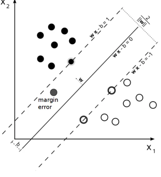
Figure2.1 shows an example of the application of the kernel trick for the classi-fication of points in a 2-dimensional space.

We will see in the following sections some examples of kernel methods.

Figure 2.1: Example of classification using the kernel tick.

2.4.1

The Perceptron algorithm

One of the oldest algorithms used in machine learning (from early 60s) is an online algorithm for learning a linear decision function (an hyperplane) on real-valued vectorial data, called the Perceptron Algorithm [14].

A prototype vector w is (randomly) initialized, and used as the decision function. An example xi is predicted as positive iff w·xi +b >0 and as negative otherwise.

The prediction is then compared with the real class of the example. On a mistake, a new prototype vector w0 is generated as w0 = w+αyixi, where 0 < α ≤ 1 is

a constant that influences the learning rate, and yi ∈ {+1,−1} is the class of the

example. This is a very simple algorithm, that guarantees to find a linear separator between positive and negative examples, if it exists.

The original algorithm has been extended in order to be applied with kernel functions, where the examples xi are substituted with φ(xi) in the formulation.

(31)

This new formulation lies on the observation thatw, after have seen a number t

of examples, is no more than a weighted sum of the examples where we have made mistakes so far, that is:

wt=αyi1xi1 +. . .+αyit−1xit+1

where xi1, . . . , xit−1 is the set of misclassified examples.

So to compute φ(w)·φ(x) we can just do:

φ(w)·φ(x) =αyi1K(xi1, x) +αyit−1K(xit+1, x)

where φ is the function that maps examples in the feature space and K the corresponding kernel function.

The examples used to define the hypothesis (i.e. the misclassified examples) are referred to assupport vectors. Perceptron findsone separator for the examples inX. The perceptron is a fast and simple algorithm that can be applied to online learning tasks. Its main drawback is that it does not provide bounds on generalization error.

2.4.2

The Support Vector Machine

One of the most important algorithms in kernel methods is the Support Vector Machine(SVM) [138].

SVM is based on the principle of structural risk minimization[139] that is an inductive principle for model selection used for learning from finite training data sets. It describes a general model of capacity control and provides a tradeoff between hypothesis space complexity (the VC dimension of approximating functions, see Section 2.4) and the quality of fitting the training data (empirical error, defined in Equation 2.1). The procedure is outlined below.

Given a class of hypotheses (in this case being the hyperplanes in the feature space defined from the adopted kernel function), divide it into a hierarchy of nested subsets in order of increasing complexity. Perform empirical risk minimization on each subset (this is essentially parameter selection). Select the model in the series

(32)

whose sum of empirical risk and VC confidence (i.e. a value that directly depends on VC dimension) is minimal.

Let us now focus on how SVM works. In a first phase, the examples are pro-jected in a feature space; then we search for a hyperplane that separate positive and negative examples maximizing the margin, that is the minimum distance between the hyperplane and the nearest example. We want to maximize the margin because VC dimension of a linear classifier can be expressed as a function of the margin. If the training set is linearly separable in the feature space, then the hyperplane that maximizes the margin, referred as optimum hyperplane, is unique and correspond to the solution of the following problem:

argmin

w,b

||w||2

2 s.t. ∀(xi, yi)∈S.yi(w·φ(xi)) +b ≥1 (2.2) where w and b define the hyperplane in the feature space. We will refer to this formulation as primal, as it is expressed in the feature space. The margin is inversely proportional to the norm ofw, so minimizing||w||2_{corresponds to selecting} the simpler hypothesis from the ones that satisfy the constraints. The representer theorem states that the solution f of the problem 2.2 can be reformulated as:

∀x∈ X.f(x) = X

xi∈S

αik(xi, x)

The examples for whichα6= 0 are called support vectors. We will refer to this formu-lation as dual since it is expressed in terms of the corresponding dual optimization problem.

In many cases we may not want to classify correctly all training examples to avoid the so-called overfitting problem, maybe for the presence of noise in the data, maybe for the high complexity of the hypothesis in the case training set is not linearly separable. More precisely, overfitting takes place when the case of the selected hypothesis has poor generalization capabilities, that is it has poor classification performance on unseen data. Intuitively, it is as if the classifier has learned by heart the training examples, so it is not able to classify correctly the new data.

(33)

It is possible to define a tradeoff between the mistakes on the training set and the complexity of the hypothesis:

argmin w,b, ||w||2 2 +C n X i=1 i s.t. ∀(xi, yi)∈S.yi(w·φ(xi)) +b ≥1−i, i ≥0, i= 1, . . . , n.

The C parameter of the SVM influences this tradeoff. The optimal value of C

depends on the problem.

The dual version of the soft-margin support vector machine can be expressed as follows: max α n X i=1 αi − 1 2 n X i=1 n X j=1 yiyjK(xi, xj)αiαj, subject to: 0≤αi ≤C, for i= 1,2, . . . , n, n X i=1 yiαi = 0

where the variables αi are Lagrange multipliers. This is the standard formulation

for the SVM.

2.5

The curse of dimensionality and dimension

re-duction

When dealing with high-dimensional data, various phenomena that do not occur in low-dimensional settings arise. This problem is known as the curse of dimensional-ity [58].

The curse of dimensionality arises from the fact that when the dimensionality of the space where learning is performed increases, the volume of this space increases so fast that the available data becomes sparse. This sparsity is problematic for any method that requires statistical significance. In order to obtain a statistically sound and reliable result, the amount of data you need to support the result often grows

(34)

exponentially with the dimensionality. Moreover, organizing and searching data often relies on detecting areas where objects form groups with similar properties; in high dimensional data however all objects appear to be sparse and dissimilar in many ways which prevents common data organization strategies from being efficient. This problem is also faced by kernel methods because of the implicit mapping in the high dimensional feature space. To address this problem in machine learning, techniques for dimensionality reduction are used, that are techniques for reducing the number of variables under consideration, i.e. for reducing the dimensionality of the space where learning is performed.

Feature selection is an example of a dimensionality reduction technique, which tries to find an informative subset of the original variables using statistical measures. Feature selection has been successfully applied to various machine learning algo-rithms. The advantages of using these techniques are the reduction of the noise in input data discarding some useless or not-correlated information (for the task), making learning from the data simpler.

In kernel methods, dimensionality reduction consists in reducing the dimension-ality of the feature space. As stated in Section 2.2 usually kernel methods perform the mapping in the feature space only implicitly, so the application of dimensionality reduction techniques in the feature space is not trivial. The study of how to extend the application of these techniques to kernel methods is an interesting research line, because various existing kernel functions may benefit from it. In Section 4.5.1 we will present feature selection techniques applicable to the problem of learning from graph data in more detail.

2.6

SVM training

2.6.1

Gradient Descent

Gradient descent (GD) is a mathematical technique for finding the minimum of a function. This method uses the fact that the gradient ∇f of a function points in

(35)

the direction of greatest increase. This means that −∇f points in the direction of greatest decrease. GD can be applied to solve the SVM optimization problem stated in Section 2.4.2. For example, if we consider the primal SVM formulation, a natural iterative algorithm to find the minimum of equation2.2, referred for clarity asfSV M,

is to update an estimate wt using wt+1 =wt−α∇fSV M(wt), where 0 < α <1 is a

learning rate (necessary for convergence) and∇fSV M(wt) is the gradient offSV M(wt)

computed on the whole training set.

2.6.2

The SMO algorithm

Sequential minimal optimization is an algorithm for efficiently solving the large optimization problem which arises during the training of support vector machines, invented by Microsoft research [110]. SMO breaks the main problem into a set of the smallest possible quadratic programming problems, which are then analytically solved. The algorithm proceeds as follows:

1. Find a Lagrange multiplierα1 that violates the Karush–Kuhn–Tucker (KKT) conditions for the optimization problem.

2. Pick a second multiplierα2 and optimize the pair (α1, α2). 3. Repeat steps 1 and 2 until convergence.

When all the Lagrange multipliers satisfy the KKT conditions (within a user-defined tolerance), the problem has been solved. Although this algorithm is guaran-teed to converge, heuristics are used to choose the pair of multipliers to accelerate the rate of convergence. The complexity of this algorithm is quadratic in the dataset size, while previous methods were cubic.

2.7

Online learning algorithms

When the amount of data to process becomes very large, kernel methods have a bottleneck related to the computational complexity of the learning algorithms. The

(36)

problem of processing huge amounts of data is receiving increasing attention. Ac-cording to a report from IDC titled “The Digital Universe in 2020: Big Data, Bigger Digital Shadows, and Biggest Growth in the far East” [64], only 0.5% of the 643 exabytes of useful data have been analyzed. Examples of this data include images, social media, sensors (including those in our smartphones and other devices, as well as those that may be implanted into the body) or medical devices. Indeed, the most popular learning algorithm, the SVM, scales quadratically in the dataset size. This complexity may be impractical when dealing with datasets of several thousands of examples. The simplest way to handle large datasets is to randomly discard data, but there are statistical benefits to process more data [19].

Recent research focused on large-scale learning, e.g. [154,28], but the majority of the methods focus on linear SVMs not allowing for the application of the kernelized formulation. Other researches slightly modify the optimization problem to make the parallelization possible [155]. Typically, the complexity of these methods remains quadratic.

A promising way to deal with large-scale datasets that has been recently proposed is to use online learning algorithms, that are learning algorithms that process one example at a time. Indeed, it is possible to apply online learning algorithms on big batch datasets, allowing for multiple (sequential) passes over the data. Typically, each complete pass over the data is referred as an epoch.

This approach is very flexible because it allows an user to adjust the tradeoff between computational time and the quality of the solution.

Moreover, even if online algorithms are in general simpler with respect to batch ones, for most of them the solution (given that some properties are respected) con-verges to the global optimum. These algorithms belong to the general family of Stochastic Gradient Descent algorithms[120], that will be presented in Section2.7.3. Unlike other approaches, in the non-kernelized version SGD has constant update time and constant space occupation.

Algorithms belonging to the SGD family can be easily kernelized to be applied to nonlinear classification problems. However, it becomes necessary to store the set of

(37)

support vectors and in general the number of SVs grows linearly with the size of the dataset. In the large-scale scenario we deal with huge datasets, thus this approach leads to the problem of exceeding the available memory and to the linear growth of the training and test times [5].

In order to face these issues, in [146] it is proposed a budgeted version of SGD, referred as BSGD (see Section 2.7.4).

2.7.1

Stream data mining

Data streams are becoming more and more frequent in many application domains thanks to the advent of new technologies, mainly related to web and ubiquitous services [11,62]. In a data stream, data elements are generated at a rapid rate and with no predetermined bound on their number. For this reason, processing should be performed very quickly (typically in linear time) and using bounded memory resources. Data streams can be viewed as ordered infinite sequences of instances, flowing at variable rates and typically produced by a non-stationary source. They can be generated for example by sensor networks, user clicks, web server connections or emails.

Moreover, every real-world classification system may take advantage of continu-ously adapting the model with a feedback from the new data.

Unfortunately, conventional knowledge discovery tools cannot manage this over-whelming volume of streaming data. The study of the issues related to the new nature of incoming data represents the starting point to understand the main fac-tors influencing the data streams problem.

Batch machine learning techniques typically require data to be entirely stored in memory, and to work with multiple passes on this data. In data streams scenario, the huge amount of data cannot be stored in memory or on disk. Thus, it’s crucial to design mining algorithms using efficient techniques to bound the time and space necessary to extract a model.

Moreover, in streaming contexts a phenomenon called concept drift frequently occurs, and makes mining data streams even more complex. Indeed, in the data

(38)

streams world the underlying concept that we are trying to learn is not stable, but constantly evolving over time [86]. For example, if we want to predict weekly merchandise sales in an online shop we can develop a predictive model that works satisfactorily. The problem is that the behavior of the customers may change over time. The model may use inputs such as the amount of money spent on advertising, promotions being run, and other metrics that may affect sales. The model is likely to become less and less accurate over time - this is concept drift. In the merchandise sales application, one reason for concept drift may be seasonality, which means that shopping behavior changes seasonally. Perhaps there will be higher sales in the winter holiday season than during the summer, for example. This problem in the classification context requires special techniques.

The main challenge of stream data mining is to accurately capture the continuous changing decision concepts and scale up to large volume of stream data. The nature of data streams requires the use of algorithms that involve at most one pass over the data and try to keep track of time-evolving features (concept drift). Summarizing, the characteristics required from online learning algorithms are:

• example processing in linear time;

• no need for storing examples after they have been processed (single pass over data);

Incremental (online) Learning

Incremental learning has recently attracted growing attention from both academia and industry. From the computational intelligence point of view, there are at least two main reasons why incremental learning is important. First, from data mining perspective, many of today’s data-intensive computing applications require learning algorithms to be capable of incremental learning from large-scale dynamic stream data, and to build up the knowledge base over time to benefit future learning and decision-making processes. Second, from the machine intelligence perspective, bi-ological intelligent systems are able to learn information incrementally throughout

(39)

their lifetimes, accumulate experience, develop spatial-temporal associations, and coordinate sensor-motor pathways to accomplish goals. We mainly focus on the first issue. Historically, inductive machine learning has focused on non-incremental learning tasks, i.e., where the training set can be constructed a priori and learning stops once this set has been duly processed, because it is the simplest learning sce-nario. There are, however, a number of areas, such as agents, where learning tasks are incremental. In recent years, the attention has been posed on this type of learn-ing (see e.g. [71]) and some work has been done for defining incremental learning systems, for example in [74] is proposed a general incremental learning framework that is able to learn from stream data for classification purpose. The traditional online learning problem can be summarized as follows. Suppose a, possibly infinite, data stream in the form of pairs (x1, y1), . . . ,(xt, yt), . . ., is given. Herext ∈Xis the

input example and yt = {−1,+1} its classification. Notice that, in the traditional

online learning scenario, the label yt is available to the learning algorithm after the

class of xt has been predicted. The goal is to find a function h : X → {−1,+1}

which minimizes the error, measured with respect to a given loss function, on the stream. There are additional constraints on the learning algorithm about its speed: it must be able to process the data at least at the rate it gets available to the learning algorithm. Moreover, the amount of memory available to represent h() is limited by memory constraints or by the user.

Concept drift

When moving from the classical batch learning scenario to the online setting, the learning problem becomes more challenging. When dealing with large amounts of data produced from data streams, the problem of extracting knowledge from the data becomes more difficult because the data distribution and the underlying concept may be subject to continuous changes. An effective stream data mining algorithm should therefore be capable of dealing with such changing concepts and producing accurate models. In practice, this issue can be addressed by detecting changes in the data streams and continuously updating the prediction models according to the most

(40)

recently arrived data.

We can characterize concept drifting in two macro classes:

• loose concept drifting;

• rigorous concept drifting;

the main difference between them being the speed in which changes in concepts happen. In the former the concept slowly changes over the time, while in the latter at a certain time t the concept changes.

2.7.2

Formalization and Feasible approaches

The most commonly used formalization for stream data mining with concept drift-ing is presented in [88] and models a stream as an infinite sequence of elements

e1, . . . , ej, . . .. We can divide a data stream into batches b1, b2, . . . , bn, . . . where

bi =ei1, . . . , ei_ni. For each batch bi, we assume data as identically distributed with

regard to a distribution Pi(e). Depending on the amount and type of concept drift,

Pi(e) will differ fromPi+1(e).

Data accumulation policy

As summarized in [74], the family of methods that adopts a data accumulation policy, simply develops a new hypothesis whenever a chunk of data is received. Thus the hypothesis ht is based on all the available data accumulated up to time t,

i.e. {b1, b2, . . . , bt}and the previously trained hypothesisht−1 is discarded. This is a too straightforward and simplistic approach for many scenarios: in fact the existing learned hypothesisht−1 is not used for the learning of the new oneht. When concept

drift happens, the learner is not able to adapt quickly to the new data. We would like to point out that for some memory-based approaches such as the locally weighted linear regression method, a certain level of previous experience can be accumulated to avoid the ”catastrophic forgetting” problem. Nevertheless, this group of methods generally requires the storage of all accumulated data items. Therefore, it may not

(41)

be feasible in many data-intensive real applications (as when we deal with examples in structured form) due to the constraints of limited memory and computational resources.

Classifier ensemble for stream data mining

Existing research in the area has proposed a set of ensemble frameworks for stream data mining. Under this framework, one can build classifiers on rather small data chunks without missing major patterns.

One of the first approaches that deals with streams of structured data, in partic-ular with trees, is proposed in [72]. The idea is not to keep in memory all examples that come from the data stream. Instead, only a fixed number of data chunks are kept in memory (e.g. the lastn chunks). A model is generated for each data chunk. When a chunk becomes outdated, it is not deleted but it is aggregated with an-other old data chunk in a DAG that is a compressed lossy representation of them, generating one single model. With this policy, we have a bounded, fixed number of models, and thus of classifiers, that are combined in a (linear) committee.

When a new data chunk arrives, there is a re-weighting phase that computes a new weight for each model based on its accuracy on a part (25%) of the current chunk. This weighting phase keeps only the informative parts of the data, thus this makes possible to deal with concept drifting. Old concepts will have a very low weight.

2.7.3

Online Stochastic gradient descent algorithms

Online algorithms to approximately solve the SVM optimization problem have been proposed in order to incrementally update the model working on a single example at a time. For example LASVM [16] proposes a tradeoff between optimality and scalability modifying the SMO algorithm to incrementally upgrade the model. Gra-dient descent methods are an appealing alternative to the quadratic programming methods. In stochastic gradient descent (SGD) the SVM training is transformed

(42)

in an unconstrained problem. The algorithm scan the data one example at a time and the model is updated using (sub-)gradient descent over an instantaneous ob-jective function. This class of algorithms, due to its iterative nature, is often run in epochs, performing multiple passes over the input data for improved accuracy. The primal version of the PA, sketched in Algorithm 1, represents the solution as a sparse vectorw. In machine learningwis often referred to as themodel. SGD differs from batch gradient descent in the way the gradient is estimated[18]. In the batch gradient descent algorithm, each iteration involves a burdening computation of the average of the gradients of the loss function ∇wL(xn, w) over the entire training set,

see Section 2.6.1. The elementary online stochastic gradient descent algorithm is obtained by dropping the averaging operation in the batch gradient descent algo-rithm. Instead of averaging the gradient of the loss over the complete training set, each iteration of the online gradient descent consists of choosing an example xt at

random, and updating the parameters wt according to the following formula:

wt+1 =wt−α∇wL(xt, wt)

whereα is the learning rate and L() is a loss function and∇wL(xt, wt) indicates the

gradient, that is the vector of partial derivatives, of L(xt, wt) with regard to w .

It is worth noticing that most online algorithms actually are stochastic gradi-ent descgradi-ent algorithms. For example, the perceptron algorithm presgradi-ented in Sec-tion 2.4.1 updates the model, when an error occurs, with the following update rule:

wt+1 =wt+ 2αytwtTxt

is a stochastic gradient descent with the following loss function

Lperceptron(x, w) = (sign(wTx)−y)wTx. (2.3)

The resulting SGD rule is:

wt+1 =wt−α(sign(wtTxt)−yt)wTtxt

Since the desired class is either +1 or -1, the weights are not modified when the pattern x is correctly classified. Therefore this parameter update rule is equivalent

(43)

Algorithm 1 Primal Stochastic gradient descent online learning.

1: Initializew:w0= [0,0, . . . ,0]

2: for each roundtdo

3: Receive an instancextfrom the stream

4: Compute the score ofxt:S(xt, wt) =wTtxt

5: Receive the correct classification ofxt:yt

6: ifL((xt, yt), Mt)>0then

7: update the hypothesis: wt+1=wt−α∇wL(xt, wt)

8: end if 9: end for

to the perceptron rule. Algorithm 1 summarizes the primal SGD procedure. When a new example xtarrives(line 3) the algorithm computes its score (line 4) by means

of a dot product with the current model wt. The prediction is thensign(S(xt, wt)).

After the prediction has been made, the correct labeling yt is received. If a

pre-diction mistake occurred and the loss function value is greater than zero (line 6), the algorithm needs to update the model accordingly (gradient descent step). The new model wt+ 1 is computed accordingly to the particular gradient descent rule

(line 7). It is worth to notice thatL(xt, wt) is the gradient of the instantaneous loss

function L defined only on the latest example. In the original SGD formulation,

L((xt, yt), wt) =max(0,1−ytS(xt, wt)) is the hinge loss function.

Note that an equivalent dual version of SGD algorithm exists. For sake of sim-plicity, we will introduce a similar dual algorithm in the next section, and the dual Budget Stochastic Gradient Descent in Section 2.7.4.

Online Passive-Aggressive

The Passive-Aggressive (PA) [39], among the different online learning algorithms,

presents state-of-the-art performances, especially when budget constraints are present [149]. In Section 5.2 we propose an extension to this algorithm that deals with structured

data. There are two versions of the algorithm, primal and dual, which differ in the way the solutionh() is represented. We will assume in the following that the model vector w is sparse. In other words, we are not going to store the whole vector w, but only the elements that differs from zero. In the following we will use |w| as the

(44)

number of non null elements in w. This assumption allows us not to work directly in the input space (the space in which examples live), but to use a mapping function

φ from the input space to another bigger vectorial space, referred as feature space. For more details about the possible mappings, see Section 2.3.

Let us define the score of an example as:

S(xt, wt) = wt·φ(xt). (2.4)

Note that h(x) corresponds to the sign of S(x). The algorithm, sketched in Algo-rithm 2, proceeds as in the stochastic gradient descent presented in Section 2.7.3: the vector w is initialized as a null vector (line 1) and it is updated whenever the sign of the scoreS(xt) of an examplext is different fromyt(line 6). The update rule

of the PA finds a tradeoff between two competing goals: preserving w as much as possible and changing it in such a way thatxtis correctly classified. In the algorithm

the weight assigned to the new example entering in the support set is referred asτt.

In [39] it is shown that the optimal update rule is:

τt= min C,max(0,1−S(xt, wt)) kxtk2 , (2.5)

whereCis the tradeoff parameter between the two competing goals above. It can be shown that Passive-Aggressive belongs to the family of stochastic Gradient Descent algorithms.

Algorithm 2 Primal Passive-Aggressive online learning.

1: Initializew:w0= (0, . . . ,0)

4: Compute the score ofxt:S(xt, wt) =wt·φ(xt)

5: Receive the correct classification ofxt:yt

6: ifytS(xt)≤1then

7: update the hypothesis: wt+1=wt+τtytφ(xt)

Under mild conditions [41], to everyφ() corresponds a kernel functionK(xt, xu),

(45)

explained in Section 2.2. Notice that w=P

i∈Myiτiφ(xi), where M is the set of

examples for which the update step (line 7 of Algorithm 2) has been performed. Then Algorithm 2 has a correspondent dual version, presented in Algorithm 3, in which the τt value is computed as

τt= min C,max(0,1−S(xt, Mt)) K(xt, xt) (2.6) and the score of equation (2.4) becomesS(xt, Mt) = P_x_i∈MtyiτiK(xt, xi).

Algorithm 3 Dual Passive-Aggressive online learning.

1: InitializeM:M0={}

4: Compute the score ofxt:S(xt, Mt) =P(xi,yi,τi)∈MtyiτiK(xt, xi) 5: Receive the correct classification ofxt:yt

6: ifytS(xt)≤1then 7: computeτt= min C,max(0,1−S(xt,Mt)) K(xt,xt)

8: update the hypothesis: Mt+1=Mt∪ {(xt, yt, τt)}

Here M is the, initially empty set of tuples corresponding to support examples which the update rule modifies as M =M∪ {xt, yt, τt}, where xt is the example, yt

its label and τt its weight computed accordingly to Equation 2.6. It can be shown

that the primal and dual algorithms compute the same solution. However, the dual algorithm does not have to explicitly represent w, since it is only accessed implicitly through the corresponding kernel function.

2.7.4

Budget online stochastic gradient descent algorithms

Respecting a memory budget is one of the constraints of online learning algorithms, as explained in Section 2.7. Moreover, if the algorithm complexity depends on the memory occupation like in the dual algorithms presented in Section 2.7.3, an effective method to control the speed of online learning algorithms is to control the amount of memory the algorithm is allowed to use. Assigning a fixed memory budget in this way ensures that the algorithm do not run out of memory, and

(46)

burden the computational complexity of the algorithm since for most of them the computational complexity can be expressed as a function of the budget. In this section we will review some of the most important algorithms in literature for this scenario.

Budget stochastic gradient descent

The paper [146] proposes a modification of SGD algorithm limiting the model size to a budget B expressed as the number of Support Vectors representing the model. A budget maintenance step is performed whenever the number of SVs exceeds the budget, namely |M| > B. This step reduces the size of M by one. The result of this step is a degradation of the classifier. The budget maintenance strategy greatly influences this degradation. In Section 2.8 some of the principal strategies are presented, including random, oldest ones and the examples having lowestτ value.

Algorithm 4 Dual Stochastic gradient descent online learning on a budget.

1: InitializeM:M0={}

4: Compute the score ofxt:S(xt, Mt) =P(xi,yi,τi)∈MyiτiK(xt, xi) 5: Receive the correct classification ofxt:yt

6: ifL((xt, yt), Mt)>0then

7: whilesize(Mt) +size(xt)>Bdo

8: select an examplejand remove it fromMt

9: end while

10: computeτt=αL((xt, yt), Mt)

11: update the hypothesis: Mt+1=Mt∪ {(xt, yt, τt)}

Let’s proceed briefly explaining the algorithm. When a new example xt

ar-rives(line 3) the algorithm computes its score (line 4) applying a kernel function with all the support vectors. Here the τ is the weight associated to each support vector (calculated in line 10). The prediction is then sign(S(xt)). After the

pre-diction has been made, the correct labeling yt is received. If a prediction mistake

(47)

to update the model accordingly (gradient descent step). At this point, if the budget

B is full, the budget maintenance step have to be performed. In this case, according to the particular policy, a support vector is removed. This step lead to a degradation of the model, that can be bounded for some budget maintenance policies. Finally, the example xt can be inserted into the model M. A new tuple is generated (line

11) containing the example, its label, and the weightτ computed accordingly to the particular gradient descent rule (line 10). It is worth to notice that L(xt, Mt) is the

gradient of the instantaneous loss function L defined only on the latest example. In the original BSGD formulation, L((xt, yt), Mt) = max(0,1−ytS(xt, Mt)) is the hinge loss function. Different works proposed modifications of the way the budget is maintained, each one giving funny names to the resulting algorithms. Most of them are briefly explained in Section 2.8. For sake of simplicity, in this chapter we will separate the learning algorithms with the budget policies.

In the next sections, we will present several learning algorithms that can be viewed as slight modifications of Algorithm 4. For this reason, where possible we will present the algorithms pointing out the differences with this one.

Budget perceptron

The simplest budget online algorithm is, not surprisingly, the budget perceptron. This modification of the original perceptron algorithm was first proposed in [40]. We can easily obtain the algorithm instantiating the loss functionL(xt, yt, Mt)

calcula-tion in lines 6 and 10 of the BSGD Algorithm4to the perceptron ruleLperceptron(xt, yt, Mt) =

(sign(S(xt, Mt)−y)ytS(xt, Mt). It is worth to notice that this rule is the same rule

presented in equation 2.3 but for the dual version of the algorithm.

Budget online Passive-Aggressive

In [149] it is proposed to modify the dual version of the passive aggressive algo-rithm presented in Algoalgo-rithm3introducing the same budget constraint as in BSGD. Recalling from Section 2.7.3, the main difference between the perceptron and the passive-aggressive algorithm is that in the former the model is updated only if a

(48)

classification mistake occurs, while in the latter the model is updated even when a

margin error occurs. In other words, we update the model even when an example is correctly classified but it is too close to the separating hyperplane (for an example, see Figure 2.2).

Figure 2.2: Example of a margin error.

For this algorithm, the loss function is computed according to Equation2.5, and looks like: L(