ISSN 1440-771X
Australia
Department of Econometrics
and Business Statistics
http://www.buseco.monash.edu.au/depts/ebs/pubs/wpapers/
Half-Life Estimation based on the Bias-Corrected Bootstrap:
A Highest Density Region Approach.
Jae Kim, Param Silvapulle and Rob J Hyndman
June 2006
Half-Life Estimation based on the Bias-Corrected Bootstrap:
A Highest Density Region Approach
Jae H. Kim1 Param Silvapulle Rob J. Hyndman
Department of Econometrics and Business Statistics Monash University, Australia
Abstract
The half-life is defined as the number of periods required for the impulse response to a unit shock to a time series to dissipate by half. It is widely used as a measure of persistence, especially in international economics to quantify the degree of mean-reversion of the deviation from an international parity condition. Several studies have proposed bias-corrected point and interval estimation methods. However, they have found that the confidence intervals are rather uninformative with their upper bound being either extremely large or infinite. This is largely due to the distribution of the half-life estimator being heavily skewed and multi-modal. In this paper, we propose a bias-corrected bootstrap procedure for the estimation of half-life, adopting the highest density region (HDR) approach to point and interval estimation. Our Monte Carlo simulation results reveal that the bias-corrected bootstrap HDR method provides an accurate point estimator, as well as tight confidence intervals with superior coverage properties to those of its alternatives. As an application, the proposed method is employed for half-life estimation of the real exchange rates of seventeen
industrialized countries. The results indicate much faster rates of mean-reversion than those reported in previous studies.
Keywords: Autoregressive Model, Bias-correction, Bootstrapping, Confidence interval, Half-life, Highest density region. JEL: CLASSIFICATION: C15,C22,F37
1 The corresponding author.
Department of Econometrics and Business Statistics, Monash University, Caulfield East, Vic 3145, Australia. Tel. (+61 3) 99031596, Fax. (+61 3) 99032007. Email. [email protected]
1. Introduction
Measuring the degree of mean-reversion or persistence in economic and financial time series has been an issue of extensive investigation (see, for example, Campbell and Mankiw; 1987, 1989). It is particularly important in the context of testing for the validity of parity conditions in international economics. For example, mean-reversion of real exchange rates is a key condition for the empirical validity of the purchasing power parity (Rogoff, 1996). The half-life, defined as the number of periods required for the impulse response to a unit shock to a time series to dissipate by half, has emerged as a popular measure of persistence in this context.
In this paper, we pay attention to half-life estimation only in the context of linear univariate autoregressive (AR) models. In the AR(1) model with the slope coefficient α, the half-life h can be calculated as h = log(0.5)/log(α). A natural estimator is
ˆ log(0.5) / log( )ˆ
h= α , where ˆα is the least-squares estimator of α. There are three
noteworthy statistical properties of ˆh. First, it has an unknown and possibly
intractable distribution. Second, it may not possess finite sample moments since it takes extreme values as ˆαapproaches one. Third, it is intrinsically biased in small samples; it is a non-linear function of ˆα which is also biased downward. It can also easily be illustrated that a tiny estimation error in ˆα can result in extreme variability of ˆh, which is the main reason for the atypical features mentioned above. For an
AR(p) model with p > 1, ˆh can be obtained from the impulse response function, and
Recent studies concerned with estimation of the half-life based on the AR model can be divided into two groups, excluding Kilian and Zha (2002) who used the Bayesian method. The first group of studies, including Gospodinov (2004) and Rossi (2005), considered alternative asymptotic confidence intervals. The second group of studies is based on the bootstrap of Efron and Tibshirani (1993) combined with a
bias-correction procedure for parameter estimators. Murray and Papell (2002, 2005) and Caporale et al. (2005) used the bias-corrected bootstrap, similar to that of Kilian (1998). Rapach and Wohar (2004) used the grid bootstrap of Hansen (1999), and so did Rossi (2005) in addition to the asymptotic methods. In this paper, we restrict our attention to the second group of studies.
To illustrate the method proposed by the second group of studies, we take the AR(1) case as an example. A bias-corrected estimator for half-life can be obtained as
ˆc log(0.5) / log( )ˆc
h = α where αˆc is a bias-corrected estimator for α. And then αˆc is
bootstrapped to approximate the sampling distribution of ˆc
h . Murray and Papell
(2002) and Caporale et al. (2005) used the Andrews-Chen (1994) approximately median-unbiased estimator for AR parameters to obtain ˆαc and ˆc
h . They calculated
the confidence intervals for half-life from the bootstrap distribution of ˆc
h obtained by
bootstrapping of ˆαc, again using the Andrews-Chen (1994) estimator for
bias-correction.
A notable feature commonly observed in the past studies is that confidence intervals for half-life are too wide and their upper bounds are often infinite2. This indicates that
2 This statement applies to the bootstrap-based and asymptotic confidence intervals mentioned above. The bootstrap confidence intervals without bias-correction and the asymptotic confidence interval
the degree of uncertainty associated with point estimates is extremely large, and the intervals are rather uninformative. This also implies that the deviations from the parity condition may be regarded as being mean-averting, and the empirical validity of the parity condition under consideration is questionable. This is a puzzling outcome, as it contradicts the view commonly held by many economists that international parity conditions should hold under some conditions. We believe that the main reason for this puzzle lies in the methods of the past studies that do not adequately address the atypical distributional properties of the half-life estimator. Clearly, there is a need for a new approach.
The primary objective of this paper is to propose a new non-parametric method for point and interval estimation of half-life. This alternative method requires: (i) the use of the bias-corrected bootstrap proposed by Kilian (1998) to approximate the
sampling distribution of ˆc
h ; (ii) estimation of the kernel density of the above bootstrap
distribution, by adopting the transformed kernel density method of Wand et al. (1991) and the data-based bandwidth selection method of Sheather and Jones (1991); and (iii) the use of the highest density region (HDR) method proposed by Hyndman (1996) for point and interval estimation of half-life. Since these new methods take account of the atypical properties of the distribution of the half-life estimator, they are expected to be superior to other bootstrap-based methods.
An extensive Monte Carlo simulation experiment is conducted to evaluate small sample properties of the HDR point and interval estimators for half-life based on the bias-corrected bootstrap. These HDR estimators are compared with the methods based
based on the delta method are too short providing coverage rates much lower than the nominal coverage. See also Rossi (2005).
on the median-unbiased estimators proposed by Murray and Papell (2002, 2005) and Caporale et al. (2005). In contrast with the latter, our bias-corrected bootstrap method does not yield a bootstrap distribution of ˆc
h with infinite elements, due to the
stationarity-correction similar to that of Kilian (1998), although it can be heavily skewed and multi-modal with extremely large values. In this situation, the HDR-based point and interval estimation is expected to provide accurate and reliable estimators. In our simulation study, we indeed find that the HDR method for estimating the half-life performs substantially better than the others. The bias-corrected bootstrap HDR estimator provides point estimates much more concentrated around the true value and tighter confidence intervals with superior coverage properties.
The bias-corrected bootstrap HDR method is applied to half-life estimation of monthly real exchange rates of 17 industrialized countries studied by Kilian and Zha (2002). In comparison with the Bayesian estimates reported in Kilian and Zha (2002), our point estimates are smaller while interval estimates are slightly wider. However, our interval estimates are much tighter and more informative than those reported in the other studies such as Murray and Papell (2002, 2005), Caporale et al. (2005) and Rossi (2005).
The paper is organised as follows. In the next section, we define the half-life in a general AR model and discuss the estimation details. Section 3 outlines the bias-correction methods used in this paper, for AR parameter and half-life estimation. The bias-corrected bootstrap for the half-life is detailed in Section 4, and the HDR method is outlined in Section 5. Section 6 presents the simulation design and results, and Section 7 an empirical application. The final section concludes the paper.
2. Estimation of the Half-Life in AR Models
We consider the stationary AR(p) model of the form
Yt = μ+ βt + α1Yt-1 + … + αpYt-p + ut, (1)
where ut ~ iid (0,σ2). The assumption of a homoskedastic error term will be relaxed
later. The AR order p is assumed to be known. For p≥ 2, equation (1) can be
re-written as
Yt = μ + βt + αYt-1 + ψ1ΔYt-1 + … + ψp-1ΔYt-p+1 + ut, (2)
where Δ = 1 – B and B is the lag operator and α= α1 +…+ αp is called the persistence
parameter. The parameters in equations (1) and (2) are related as follows:
α1 = α+ψ1, αj = -ψj-1+ψj for 2 ≤j≤p-1, and αj = -ψj-1 for j = p. (3)
The above AR model can be expressed as an MA(∞) model with the coefficients
{ }
φi i 0∞
= where φ0 = 1 and φi represents the impulse response of Yt+i to a unit shock in ut at time t, i.e. φi = ∂Yt+i/∂ut , for i = 0, 1, 2, … . The plot of
{ }
0m i i
φ = against i, for a
reasonably large integer m, is called the impulse response function of Y, which
describes how a time series responds to a unit shock in the error term over a time period of length m. The half-life h is calculated as the largest value j which satisfies
|φj-1| ≥ 0.5 and |φj | < 0.5. As mentioned before, a closed form solution exists in the
AR(1) case, i.e., h = log(0.5)/log(α). For an AR(p) model with p > 1, the value of h
can be obtained from
{ }
m0 i iφ = . When j is a number between i-1 and i, linear
Given the observed time series n t t Y } 1
{ = , the least-squares (LS) estimator for γ = (μ, β, α1,…,αp) in equation (1) can be obtained by regressing Yt on (1, t, Yt-1,…,Yt-p). The
LS estimator and the associated residuals are denoted as γˆ=( , , ,...,μ β αˆ ˆ ˆ1 αˆp)and
{ }
n p t tuˆ = +1 respectively. The LS estimator for the parameters in equation (2) can be
obtained in a similar way. Note thatαˆ =αˆ1+...+αˆp. In the AR(1) case, the half-life is estimated as 1 1 ˆ ˆ log(0.5) / log( ) if < 1 ˆ otherwise h= ⎨⎧ α α ∞ ⎩ .
Note that ˆh is median-unbiased if αˆ1is median-unbiased. Although this mapping does
not work for a higher order AR model or for mean-unbiased estimation, this has motivated past studies to use bias-correction for half-life estimation.
For a higher order model, ˆh is obtained from the estimated impulse response function
{ }
ˆ m1 ii
φ
= , where ˆφi is the ith MA(∞) coefficient associated with ˆγ . When the model has a characteristic root close to one, ˆh may not be found even with a reasonably large
value of m, since
{ }
1 ˆ m i i φ= declines fairly slowly. In this case, we use an approximation
ˆ ˆ log(0.5) / log( ) if < 1 ˆ otherwise h= ⎨⎧ α α ∞ ⎩ ,
following Murray and Papell (2002)3. In this paper, we set m = n and use this
approximation if
{ }
1 ˆ n i i φ= does not reach 0.5 for i ≤n.
3 This approximation generally under-estimates the true value because the half-life is calculated as if the true model were an AR(1). However, since this approximation is used only when hˆ > n, the degree
of under-estimation should not be substantial. See Rossi (2005) for alternative approximate formulae for the half-life of a high order AR model.
3. Bias-Corrected Parameter Estimation
This section provides a review of alternative bias-correction methods for ˆγ to be used in this paper. As mentioned earlier, bias-correction of ˆγ may lead to a more accurate half-life estimator. In their empirical studies, Murray and Papell (2002) and Caporale et al. (2005) used the Andrews-Chen (1994) estimator for γ for this purpose. In this paper, the bootstrap bias-corrected estimator and the Roy-Fuller (2001) estimator are also used.
3.1. The Bootstrap Bias-Corrected Estimator
The bootstrap (Efron, 1979) is a computer-intensive method of approximating the unknown sampling distribution of a statistic, and it involves repeated resampling of the observed data. It has been applied widely in econometrics and statistics when analytical derivation of the distribution of a test statistic is intractable, and found to generate distributions very close to the underlying true distributions; see Li and Maddala (1996) and Berkowitz and Kilian (2000) for details. In the context of AR models, the bootstrap can be conducted by resampling the residuals and generating a large number of pseudo-data sets following the AR recursion using the estimated coefficients. This is done to replicate the dependence structure present in the underlying time series.
The biases of AR parameter estimators can be estimated using the bootstrap in the following way. Generate a pseudo-data set n
t t Y*} 1 { = as * * * * 1 1 ˆ ˆ ˆ ˆ ... t t p t p t Y = +μ β αt+ Y− + +α Y− +e , (4)
using { }p1 t t
Y = as starting values, where et* is a random draw with replacement from
{ }
n p t tuˆ = +1. Throughout the paper, the LS residuals are rescaled for resampling as
illustrated in MacKinnon (2000; p620). The above process can be repeated many times so that B1 sets of pseudo-data are generated, from which B1 sets of bootstrap parameter estimates for γ, denoted * 1
1
{ ( )}B j
j
γ = , can be obtained. A typical γ*= (μ*,β*, α1*,…,αp*) is obtained by regressing Yt* on (1, t, Yt*−1,...,Yt*−p). The bias of γˆ can be estimated as Bias(γˆ ) = γ*−γˆ, where γ*is the sample mean of {γ*(j)}Bj=1. It is well
known that the bootstrap estimator of bias obtained in this way converges in probability to zero at the rate of n-1 when α< 1 under certain conditions; see, for
example, Bose (1988). The bias-corrected estimator γˆBc =(μ β αˆBc, ˆBc, ˆ1,cB,...,αˆp Bc, )for γ
can be calculated as ˆγ −Bias( )γˆ .
The above bias-correction can push the parameter estimates to the non-stationary part of the parameter space. In this case, a method similar to the stationarity-correction proposed by Kilian (1998) is adopted4. This procedure can be described as follows: if
ˆc B
γ implies non-stationarity, then let δ1 = 1, Δ1 =Bias(γˆ) and ˆγBic = − Δγˆ i. Set
i i i = Δ
Δ +1 δ , δi+1 = δi – 0.01 for i = 1, 2, 3, … . Iterate until γˆ satisfies the condition ic
of stationarity and set ˆc ˆc
B Bi
γ =γ . For example, in the AR(1) case, if αˆ1= 0.95 and
4 When the initial parameter estimate has a unit or an explosive root, Kilian’s (1998) procedure does not give any adjustment. Our approach is different in that the above correction is applied to the initial estimate even when it has a unit root or an explosive root. This is to ensure that all bootstrap replicates of half-life are finite so that kernel density estimation is possible in order to implement the HDR method (see Section 5). This variation has little impact on the overall results because, given the parameter space of interest in this paper, the occurrence of an initial estimate being non-stationary is rare or non-existent in repeated sampling. If a parameter estimate with a unit or an explosive root is encountered in practical applications, the half-life estimate is infinite and the bias-corrected bootstrap test will not be conducted.
1,
ˆc B
α =1.05 with Δ1 = -0.1, then αˆ1,cBis adjusted to 0.9948, which is the outcome of
0.95+0.1 0 (1 0.01 ) l i i = −
∏
for l sufficiently large such that the value of ˆ1,c Bα is smaller than 1 (l =11 in this case). The half-life estimator obtained from ˆγBc is denoted as ˆhBc.
Note that ˆc B
h < ∞ as a result of stationarity-correction.
3.2. Roy-Fuller Estimator
The Roy-Fuller estimator provides a simple modification to the LS estimator for α in equation (2). Let ˆc min( ,1)
R
α = α , where α=α+[Cp(τˆ1)+C−p(τˆ−1)]σˆ1, α is the LS estimator for the coefficient of yˆt−1 in the regression ofyˆ on t yˆt−1,Δyˆt−1,...,Δyˆt−p+1,
whereyˆ is the LS residual from the regression of t Yt on (1, t) and σˆ1is the standard error of α. Note that τˆ1=(α−1)σˆ1−1is the unit root test statistic and τˆ−1 is the statistic
to test for the hypothesis that α = –1. The functions Cp(τˆ1) and C-p(τˆ−1) control the
way in which bias-correction is conducted, and are constructed so that ˆc R
α is approximately median-unbiased at α= 1 and –1.
Roy and Fuller (2001) suggested the following form of Cp(τˆ1) function, which is related to the bias expression for αˆ they derived:
1 1 1 1 1 1 1 1 1 1 1 0.5 1 1 1 0 5 1 ˆ (ˆ ) if ˆ ( ˆ) 3[ˆ (ˆ )] if ( )ˆ ˆ ( ˆ) 3[ ]ˆ if (3 ) 0 if ˆ (3 ) .
MED n MED MED
p MED p p d I n k K K C I n n K n τ τ τ τ τ τ τ τ τ τ τ τ τ τ τ ⎧ ⎪ ⎪ − − ⎪ ⎪ ⎨ − − ⎪ ⎪ ⎪ . ⎪ ⎩ − + − > ; − + + − < ≤ ; = − − < ≤− ; ≤ −
where Ip is the integer part of 0.5(p+1), τMED is the median of the limiting distribution
of τˆ1 when α= 1, and =[3 − 2 ( + )][ ( + )( + )]−1 n I K n I n
of K and dn are set to 5 and 0.290, as suggested by Roy and Fuller (2001)., as
suggested by Roy and Fuller (2001). The function Cp(τˆ1) determines the magnitude of
bias-correction, as a smooth and increasing function of the unit root statistic τˆ1. The
function C-p(τˆ−1) is constructed in a similar manner. However, as nearly all economic
and business time series take the value of αclose to one, the value of C-p(τˆ−1) is
practically zero for economic and business time series. Further details on the Cp(τˆ1) and C-p(τˆ−1) functions are given in Roy and Fuller (2001).
Once the value of ˆc R
α is found, (μ, β, ψ1,…,ψp-1) can be estimated by regressing Yt
− ˆc R
α Yt-1 on 1, t, ΔYt-1,…, ΔYt-p+1). The value of μis restricted to be zero when ˆαRc = 1.
The parameter estimators for model (2) based on the Roy-Fuller estimator can be converted to those for model (1) using the relationships given in (3). They are denoted as ˆc (ˆc, ˆc, ˆ1,c ,..., ˆc, )
R R R R p R
γ = μ β α α . The half-life estimator obtained from ˆc
R
γ is denoted as ˆc
R
h . Note that ˆhRc can take the value of infinity since ˆαcR can take the value 1.
3.3. Andrews-Chen Estimator
Let m(α) be the median function of αˆ which is strictly increasing over the parameter
space of α ∈ (–1,1]. Then, the Andrews-Chen estimator ˆc A α of αis given by 1 ˆ 1 if (1); ˆ ˆ ( ) if ( 1) (1); ˆ ˆ 1 if ( 1); c A m m m m m α α α α α − > ⎧ ⎪ =⎨ − < ≤ ⎪− ≤ − ⎩
where m(−1) = limα→−1 m(α) and m−1 is the inverse function of m(α). This median function can be computed using the Monte Carlo simulation method described in Andrews and Chen (1994, p.192). As the simulation method can calculate the m(α)
function over a grid of αvalues in the interval (–1,1], linear interpolation is conducted to approximate the value of m−1(αˆ ), as suggested by Andrews (1993, p.146). Note
that this estimator is exactly median-unbiased for the AR(1) model, but approximately median-unbiased for the AR(p) model with p > 1 (for details, see Andrews and Chen,
1994).
Once the value of ˆc A
α is found, (μ, β, ψ1,…,ψp-1) are estimated by regressing Yt
− ˆc A
α Yt-1 on (1, t, ΔYt-1,…, ΔYt-p+1). As with the Roy-Fuller estimator, the value of μis
set to zero when ˆc A
α = 1. The above procedure can be iterated until convergence, as described in Andrews and Chen (1994, p.191). The parameter estimators for model (2) obtained in this way can be converted to those for model (1) using (3), and they are denoted as ˆ (ˆ , ˆ , ˆ1, ,..., ˆ , )
c c c c c
A A A A p A
γ = μ β α α . The half-life estimator obtained from ˆc
A γ is denoted as ˆc A h . Similarly to ˆc R h , ˆc A h ≤∞ since ˆc A
α can take the value 1.
4. Bias-Corrected Bootstrap Confidence Intervals for Half-Life
This section describes how bias-corrected confidence intervals for half-life can be obtained, using the bias-corrected estimators outlined in the previous section. The bootstrap procedure, given in three stages as below, is similar to that of Kilian (1998).
Stage 1:
Compute c ( ,c c, 1c,..., c)
p
γ = μ β α α , a bias-corrected estimator for γ, and the associated residuals
{ }
1 n c t t p u = + . Stage 2:Generate pseudo-data sets recursively as * * * * 1 1 ... , c c c c t t p t p t Y =μ +β +α Y− + +α Y− +v (5) using { }p1 t t
Y = as starting values, where v*t is a random draw with replacement from
{ }
c n 1t t p
u
= + . Using this pseudo-data series
{ }
n t t
Y* =1, the parameters of the AR(p) model are
estimated using the bias-corrected estimator used in Stage 1 and they are denoted as
* * * *
1
( c , c , c ,..., c )
p
μ β α α . The associated half-life estimate is denoted as h*.
Stage 3:
Repeat Stage 2 many times, say B2, to obtain the bootstrap-based distribution of the
half-life estimates
{ }
* 2 1. B i ih
= The confidence interval for the true half-life in the AR(p) model, based on the percentile method (Efron and Tibshirani, 1993) with nominal coverage rate 100(1-θ)%, is calculated as [ ( ), (1* * )]
h τ h −τ , where h*( )τ is the 100τth percentile of
{ }
* 2 1 B i i h = and τ= 0.5θ.Remark 1: Use of the bootstrap bias-corrected estimator
If ˆc B
γ is used in Stages 1 and 2 above, * * * *
1
( c , c , c ,..., c )
p
μ β α α in Stage 2 is calculated
using the bias estimates obtained in Stage 1, following Kilian (1998). Due to stationarity-correction, all elements of
{ }
* 21 B i i
h
= are finite (see footnote 4). The percentile interval [ ( ), (1* * )]
h τ h −τ in Stage 3 always has a finite upper bound,
although it can be excessively wide when the model is close to unit root non-stationarity.
As in Murray and Papell (2002) and Caporale et al. (2005), an approximately median-unbiased estimator may be used in Stages 1 and 2 above. Since these two estimators can yield parameter estimates with a unit root,
{ }
* 21 B i i
h
= may contain infinite elements and the percentile interval [ ( ), (1h* τ h* −τ)] in Stage 3 can possess infinite upper
bound. If ˆc A
γ is used, we use the median function obtained in Stage 1 to calculate
* * * *
1
( c , c , c ,..., c )
p
μ β α α in Stage 2 to reduce the computational burden.
Remark 3: Conditionally heteroskedastic error terms
When the error term shows departure from i.i.d., the validity of the above procedure is questionable. Many economic and financial time series are non-i.i.d., with conditional time-varying heteroskedasticity present, and the bootstrap procedure described above must then be modified. When ut is conditionally heteroskedastic, the above
procedures are modified as follows:
1. Use of the bootstrap bias-corrected estimator
If ˆc B
γ is used in Stages 1 and 2, we use the wild bootstrap that involves generating
* ˆ
t t t
e =ηu in (4) and νt*=ηtutcin (5), where ηt is any random variable with zero mean
and unit variance. Gonclaves and Kilian (2004) proved the asymptotic validity of this (recursive-design) wild bootstrap procedure for the stationary AR model. Note that our choice of ηt in this paper is the standard normal distribution.
2. Use of the Andrews-Chen or Roy-Fuller estimators
In Stage 1, no modification is given to the calculation of ˆc A
γ or ˆc R
γ . This is because, according to simulation results reported in Andrews and Chen (1994) and Roy and Fuller (2001), these estimators are reasonably robust to conditionally heteroskedastic
errors. However, in Stage 2, we conduct the parametric bootstrap by generating * t
ν in (5) as a random draw from a normal distribution, following Murray and Papell (2002).
As stated in Remark 1,
{ }
* 2 1 B i ih
= obtained using the bootstrap bias-corrected estimator does not contain infinite members. However, this distribution can be heavily skewed with extreme values and is sometimes multi-modal. When the distribution has such features, the usual percentile method is not optimal. We propose a method of
constructing a confidence interval for the half-life by estimating the distribution non-parametrically and computing the highest density region (HDR) using the algorithm given in Hyndman (1996).
5. HDR Point and Interval Estimators for Half-Life
Let f(x) be the density function for a random variable X. The 100(1-θ)% HDR is
defined (Hyndman, 1996) as the subset R(fθ) of the sample space of X such that R(fθ)
= {x: f(x) ≥fθ}, where fθ is the largest constant such that Pr[X∈R(fθ)] ≥ 1 - θ. Thus, R(fθ) represents the smallest region with a given probability content. It can take
disjoint intervals when the underlying distribution is multi-modal. It consists of the intervals associated with the modes of the distribution, while the percentile interval is centred on the median. In the present context, X is the half-life estimator of a time
series and its density can be estimated from the bootstrap replicates of the half-life
{ }
* 2 1 B i ih
5.1 Kernel Density Estimation
We estimate the density f(x) using a kernel estimator with the Gaussian kernel, with
bandwidth selected using the Sheather-Jones (1991) rule. We observe that the bootstrap distribution is heavily skewed, especially when the AR model has a root close to 1, in which case the kernel density estimation of f(x)can cause problems due
to the uneven amount of smoothing required (The long tail will be under-smoothed and modes will be over-smoothed). One way of overcoming these problems is to use the transformation kernel density estimator proposed by Wand et al. (1991). To describe this method, let Y = t(X), where t is an increasing, differentiable function on
the support of f(x). The transformation t is chosen so that the density function of Y,
denoted g(y), can easily be estimated using the standard kernel density estimation
method. From the kernel density of g(y), that of f(x) can readily be obtained using the
relationship f x( )=g t x t x( ( )) '( ).
Wand et al. (1991) proposed a general class of convex transformations called the shifted power family when f is an extremely skewed distribution. In this paper, we use
a special case t(X) = X0.1 which we have found to be the most suitable in the present
context. In the preliminary analysis, we have tried other transformations such as t(X)
= X0.3 and t(X) = X0.5, but they give kernel density estimates which are rough in the
tails and over-smoothed in the peaks. This tendency of kernel density estimates gets stronger as the value of the transformation exponent increases. We have found that the transformation t(X) = X0.1 gives the best balance in allowing sharp resolution in the
5.2.Half-Life Estimation
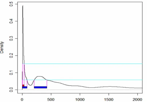
To illustrate the HDR based method for estimating the half-life, we present an example based on generated data. Figure 1 shows a transformed kernel density estimate of
{ }
* 21 B i i
h
= , calculated from a realization of the AR(1) model with α1 = 0.95, β = 0, and n = 300 under the standard normal error term, setting B1 = 500 and B2 = 2000. It is clear that the distribution is heavily skewed and bi-modal. The true value of half-life h in this case is 13.51. The sample estimates are αˆ1 = 0.92, ˆh=7.97, αˆ1,cB= 0.94
and ˆc B
h = 11.33. The upper horizontal line corresponds to f0.25 and the lower to f0.1. The
associated HDR R(f0.25) is the interval [3.8, 34.5] and R(f0.1) consists of two disjoint
intervals [2.9, 82.7] and [208.5, 425.6]. The global mode of
{ }
* 2 1 B i ih
= is 12.8. There are two points worth noting. First, the use of a bias-corrected AR coefficient improves the accuracy of half-life estimation, as ˆc
B
h provides an estimate closer to the true value of
13.51 than ˆh. Second, the HDR is substantially shorter than the percentile intervals,
which are [5.5, 125.2] and [4.2, 484.8] respectively for 75% and 90% probability coverage.
HDR Point Estimator
In this paper, we propose the use of the global mode as the HDR point estimator for half-life, denoted as ˆhHDR. We argue that the global mode is economically significant
as it is (almost always) associated with the true value of the half-life, while other modes are by-products of bias-correction and near non-stationarity. In the above example, ˆhHDR = 12.8, which is closer to the true value than ˆhBc.
HDR* Interval Estimator
We propose the use of the HDR interval associated with the global mode, which we call the HDR* interval. When the HDR consists of disjoint intervals, the HDR* represents the interval associated with the global mode. We again argue that the HDR* interval is economically significant because it provides a tight interval that covers the true value of the half-life with high coverage probabilities. In our example given in Figure 1, 75% and 90% HDR* intervals are respectively [3.8, 34.5] and [2.9, 82.7]. The second interval of 90% HDR, associated with a local mode, is not included in the HDR*.
In the next section, we conduct Monte Carlo experiments to justify our proposals for ˆ
HDR
h and the HDR* interval in repeated sampling.
6. Simulation Design and Results 6.1 Experimental Design
We consider AR(1) and AR(2) models of the form
(1 - λL) Yt= μ+ βt + ut and (1 - λL)(1 - 0.5L) Yt = μ + βt + ut ,
with λ = {0.7, 0.9, 0.95} and ut ~ iid N(0,1). Corresponding to the values of λ, the true
half-life values are {1.96, 6.58, 13.51} for AR(1) and {5.07, 14.28, 28.08} for AR(2). These AR time series are generated with zero initial values, allowing for 50 pre-sample observations. For all cases, the values of μand βare set to zero, but treated as unknowns for estimation. The sample sizes considered are 100 and 300. The numbers of bootstrap iterations B1 and B2 are set respectively to 500 and 2000, while the
number of Monte Carlo trials is set to 1000. We also consider a GARCH(1,1) error term
ut ~ N(0, σt2) with 2 2 2 1 1 0.01 0.75 0.2 t t ut σ = + σ − + − ,
to evaluate the properties of alternative half-life estimators, when the AR model has a conditionally heteroskedastic error term (see Remark 3). However, only the results associated with ut ~ iid N(0,1) are reported throughout because qualitatively similar
results are obtained under the GARCH(1,1) errors.
For point estimation, we compare the properties of ˆh, ˆhAc, ˆhRc, ˆhBc and ˆhHDRc . We use
the absolute error as a means of comparison, which is the absolute value of the difference between the point estimate and true value. For interval estimation, the properties of bias-corrected bootstrap HDR and HDR* intervals are compared with those of bias-corrected bootstrap percentile intervals obtained with the Roy-Fuller, Andrews-Chen and bootstrap bias-corrected estimators. We evaluate the coverage rate and length of confidence intervals, the former being the proportion that the interval covers the true value in repeated sampling. The nominal coverage (1-θ) is set to 0.75 and 0.90.
6.2 Comparison of the Point Estimators
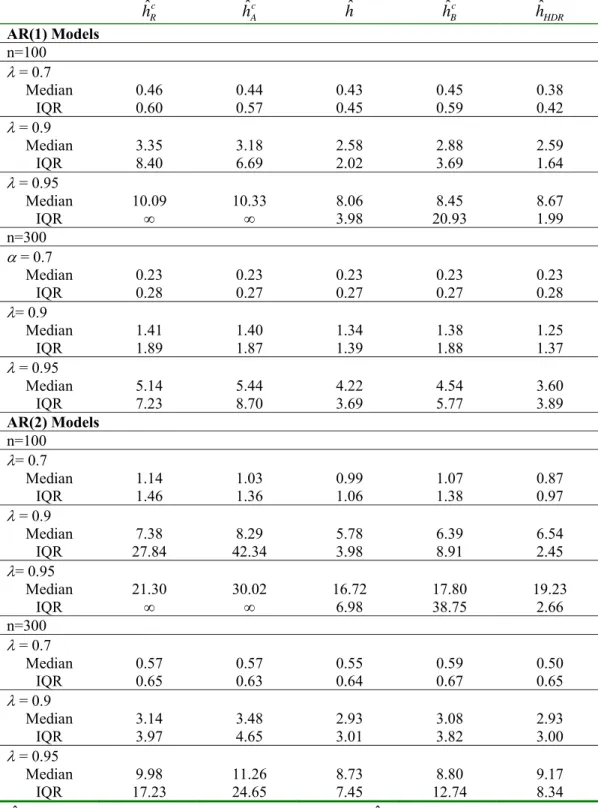
The results of point estimation are tabulated in Table 1. We report the median and inter-quartile range (IQR) of the absolute errors, since occurrence of extreme or infinite half-life estimates is possible. When λ= 0.7, all estimators show similar performances for both AR(1) and AR(2) models, although the HDR estimator performs slightly better than the others in most cases. As the value of λ increases, however, the superiority of the HDR estimator becomes evident, as it has smaller median and IQR values in most cases. The only exception occurs when λ= 0.95 and n
= 300 for the AR(2) model, where ˆc HDR
h is clearly inferior to ˆh. The overall result
indicates that ˆc HDR
h shows the best performance and should be preferred to the others
in practice, especially when the sample size is small.
There are two other points worth noting from Table 1. First, for all cases, the accuracy of half-life estimation improves with sample size, but deteriorates with a higher degree of persistence, as might be expected. Second, it is found that ˆh performs better
than ( ˆc A
h , ˆhRc, ˆhBc). This indicates that bias-correction of AR parameter estimates only
does not always improve the accuracy of point estimation. These three bias-corrected estimators tend to over-estimate the true value of half-life with a high proportion of extreme or infinite estimates, while ˆh tends to under-estimate.
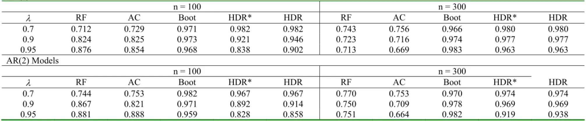
6.3 Comparison of the Interval Estimators
Table 2 reports the mean coverage rate of confidence intervals. When the Roy-Fuller and Andrews-Chen estimators are used for bias-correction, the mean coverage rates are reasonably close to the nominal rate overall. When the bootstrap bias-corrected estimator is used, the percentile, HDR and HDR* intervals show mean coverage rates much higher than the nominal rate. In most cases, the mean coverage rate is more than 90%. The HDR and HDR* intervals have the same mean coverage rate in most cases. The HDR* interval has only slightly lower mean coverage rate than the HDR interval when λ≥ 0.95. This indicates that the HDR* interval has coverage rate much higher than the nominal value, covering the true value more than 90% in most cases.
5 This difference represents the proportion of the cases where the true value of the half-life is covered by a HDR interval not associated with the global mode. This proportion is fairly small, meaning that, when the HDR covers the true value, it is almost always contained in the HDR* interval.
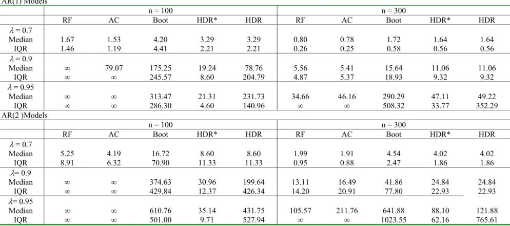
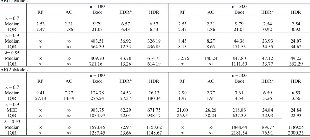
Tables 3 and 4 report the length of alternative confidence intervals for the nominal rates 0.75 and 0.90. The median length and IQR values are again reported because some of the intervals may often possess extreme or infinite length. When λ= 0.7, the confidence intervals based on the Roy-Fuller and Andrews-Chen estimators perform better than the others, with slightly shorter median length and smaller IQR values than the others. However, as the value of λincreases, these intervals become excessively wide and many of them have a high proportion of infinite upper bounds. This property is reflected in infinite median length and IQR values in Tables 3 and 4, which occur frequently when λ≥ 0.9. The bias-corrected bootstrap percentile and HDR intervals show similar features; these intervals also have median length and IQR values which increase rapidly as the value of λincreases. In contrast, the bias-corrected bootstrap HDR* interval has substantially shorter median length and smaller IQR values for nearly all cases, especially when the value of λ is closer to one and the sample size is smaller.
6.4 Further Simulation Results
Although the details are not reported for brevity, we have also simulated the AR(1) and AR(2) models with λ= 0.975. We found that the HDR point estimator and HDR* interval estimator show desirable properties similar to those reported above. The only exception was the case of the 75% confidence interval for a sample size of 100 where the mean coverage rate was substantially lower than the nominal rate. Hence, when the model has a characteristic root extremely close to one and the sample size is small, we recommend the use of the 90% confidence interval.
In practical applications, it is often the case that an AR model with the order higher than two is fitted. Although the results presented so far are suggestive, it would be more assuring if we can demonstrate that similar results can be obtained from a high order AR model. For this purpose, we have conducted a Monte Carlo experiment using an AR(12) model. The coefficients estimated from fitting an AR(12) model to a set of monthly UK real exchange rate series (see Section 7 for data details) are used as the data generation process. These AR(12) coefficients yields the value of the
persistence parameter α equal to 0.96, and the true value of the half-life obtained from the implied impulse response function is 20.61 (or 1.72 in years). Under the same simulation settings as before, the results obtained are qualitatively similar to those of the AR(1) and AR(2) models. For example, when ut ~ iid N(0,1) and n = 300, the 75%
HDR* confidence intervals have the mean coverage rate of 0.97, and the median and IQR of their lengths are 63.39 and 38.14 (or 5.28 and 3.18 in years) respectively. As for point estimation, the median and IQR values for the absolute error of ˆhHDR are
4.86 and 3.26 respectively.
We have conducted additional simulations to examine the sensitivity of the Monte Carlo results to different values of μ, β and σ in equation (1). We have found the results to be qualitatively no different from those reported in this paper. We have also simulated with alternative GARCH error specifications in the AR model such as
2 2 2
1 1
0.01 0.95 0.04
t t ut
σ = + σ − + − . Again, the results are found to be similar.
6.5 Summary and Discussion
The bias-corrected bootstrap HDR method proposed in this paper provides an interval estimator with highly desirable properties, generating tight intervals that possess
coverage rates much higher than the nominal value, even when the AR model has a characteristic root close to one. It also provides a highly accurate point estimator for the half-life. In contrast, it is evident that other bias-corrected methods based on a median-unbiased parameter estimator exhibit clearly inferior performances for both point and interval estimation6. Based on these findings, we state that the bias-corrected bootstrap HDR method should be preferred in practice for estimating the half-lives of economic and financial time series.
An interesting feature of the HDR* confidence interval is that its mean coverage rates in repeated sampling are much higher than the nominal level. This means that,
although they are tighter than competing methods, the HDR* intervals provide overly conservative assessment on the true value of half-life. This suggests that it may be possible to find a way in which the HDR* intervals are further tightened so that their mean coverage rates are reasonably close to the nominal level. One may explore analytic bias-correction based on asymptotic approximation as an alternative to bootstrap bias-correction. However, this point is beyond the scope of the present paper and is left for future research.
7. Application
We applied the bias-corrected bootstrap HDR method studied in this paper to the real exchange rates of 17 industrialized countries. The countries are listed in the first
6 As mentioned earlier, Rapach and Wohar (2004) and Rossi (2005) used the grid bootstrap of Hansen (1999) for half-life estimation. Although not examined in our simulation study, we expect that the grid bootstrap confidence interval would exhibit similar small sample properties to those of bias-corrected bootstrap intervals based on the Andrews-Chen (1994) and Roy-Fuller (2001) estimators. This is because the grid bootstrap may also yield infinite half-life estimates. Not surprisingly, the grid bootstrap confidence intervals for half-life reported in Rapach and Wohar (2004) and Rossi (2005) have infinite upper bounds for all cases they considered.
column of Table 5. The data used are monthly from 1973:01 to 1997:04, and have been analysed by Kilian and Zha (2002) for half-life estimation based on the Bayesian method. Kilian and Zha (2002) formed a consensus prior on the half-life of the real exchange rate based on a survey of economists, and then computed the posterior using a Markov-Chain Monte Carlo method. From this posterior distribution, they obtained point and interval estimates for half-life.
The estimated AR orders are reported in Table 5. For each series, we have taken a simple-to-general approach for order selection, using the Ljung-Box portmanteau and Breusch-Godfrey LM tests for serial correlation. The residuals of each series are further subject to the LM test for ARCH effect, White’s test for heteroskedasticity, the Jarque-Bera test for normality, and the CUSUM test for parameter stability. The outcomes of these tests are summarized in Table 5. It is found that the residual of a number of real exchange rates are possibly conditionally heteroskedastic. For these rates, we have used the bias-corrected bootstrap HDR method based on the wild bootstrap (Remark 3). The numbers of bootstrap iterations B1 and B2 were set
respectively to 500 and 10000.
We report the bias-corrected bootstrap HDR point estimates and HDR* confidence intervals for half-life in Table 5. To facilitate the comparison with the Bayesian results reported in Kilian and Zha (2002, Table III), 68% and 90% confidence intervals are reported. The estimates based on the other bias-corrected bootstrap methods evaluated in the previous section are not included as they are found to be clearly inferior, as might well be expected from the results reported in Murray and Papell (2002) and Caporale et al. (2005). For example, 68% and 90% bias-corrected
bootstrap confidence intervals based on the Andrews-Chen and Roy-Fuller estimators have infinite upper bounds for all rates. Figure 2 plots the density estimate for the half-life (in months) of the UK real exchange rate as an example. The HDR point estimate is 2.15 years (or 26.28 months) associated with the global mode. The upper horizontal line corresponds to f0.32 and the lower one to f0.1, and the corresponding
68% and 90% bias-corrected bootstrap HDR* confidence intervals are respectively [0.88, 6.39] and [0.44, 13.89] in years.
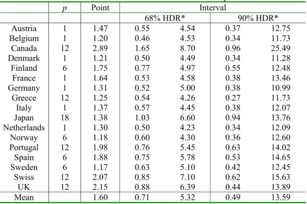
From Table 5, it can be seen that the HDR point estimates are fairly small and show a low variability, while the HDR* confidence intervals are tight. The HDR point estimates are between 1.17 and 2.89 with a mean of 1.60, which are smaller than the point estimates (posterior medians) reported in Kilian and Zha (2002) that yielded a mean value of 4.00. They are also less than the 3–5 year range that Rogoff (1996) observed from past studies. This indicates that our HDR point estimates imply a faster rate of adjustment of the deviation from the purchasing power parity than the speed of adjustment documented as a stylised fact in the literature. These short half-life
estimates are consistent with those reported in a recent study by Kim (2005), who adopted a structural error correction model approach. Our HDR* intervals are slightly narrower than the Bayesian intervals reported in Kilian and Zha (2002). For example, the mean values of the lower and upper bounds for the 68% HDR* intervals are [0.71, 5.32], while those of Kilian and Zha (2002) are [2.4, 7.5]; and those of 90% HDR* intervals are [0.49, 13.59] in comparison with [1.9, 15.1] of Kilian and Zha (2002). It is interesting to observe that all of the HDR* confidence intervals cover the 3–5 year range.
8. Conclusion
Estimation of the half-life of economic and financial time series such as real exchange rates and real interest rates has attracted much attention recently. Several studies have attempted to produce bias-corrected point and interval estimates of the half-lives using a linear AR model (see, for example, Murray and Papell, 2002, 2005; Rapach and Wohar, 2004; Caporale et al., 2005). There are two issues that motivated this study. First, the small sample properties of the bias-corrected point and interval estimators proposed by past studies are unknown. Second, past studies reported excessively wide and uninformative confidence intervals. This paper contributes to the current body of the literature on half-life estimation by examining the small sample properties of alternative point estimators. More importantly, this paper has proposed a new point and interval estimator based on the bias-corrected bootstrap of Kilian (1998) and the HDR method of Hyndman (1995, 1996). The latter provides a sensible method of point and interval estimation when the underlying distribution shows atypical properties such as extreme skewness or multi-modality.
We have conducted a Monte Carlo simulation experiment to compare the small sample properties of the bias-corrected bootstrap HDR point and interval estimators with those based on the Roy-Fuller (2001) and Andrews-Chen (1994) estimators. It is found that the bias-corrected bootstrap HDR method provides the most accurate point estimator, while the interval estimator provides tight and informative confidence intervals with coverage rate much higher than the nominal value. The results obtained in this study strongly suggest that the use of the bias-corrected bootstrap HDR method be recommended in practice when half-life is estimated for economic and financial
time series. The results of an empirical application to half-life estimation for the real exchange rates of 17 industrialized countries further support our claim.
Acknowledgements
We would like to thank Rob Brooks, Brett Inder, and Lutz Kilian for useful comments on an earlier version of the paper. Earlier stages of the paper were presented via seminars at Monash University, University of Warwick (UK), and Victoria University (Canada), and at the 3rd World Congress on Computational Statistics and Data Analysis. Constructive comments from two referees are gratefully acknowledged.
Figure 1. An example of density estimate of bootstrap distribution of half-life with 75% and 90% highest density regions.
Note: The distribution is generated from a realization of the AR(1) model with α1 = 0.95 and n = 300 under the standard normal error term.
Figure 2. Density estimate of bootstrap distribution of half-life with 68% and 90% highest density regions for the UK real exchange rate.
Table 1. Summary Statistics for the Absolute Error of Alternative Point Estimators ˆc R h ˆc A h hˆ ˆc B h hˆHDR AR(1) Models n=100 λ = 0.7 Median 0.46 0.44 0.43 0.45 0.38 IQR 0.60 0.57 0.45 0.59 0.42 λ = 0.9 Median 3.35 3.18 2.58 2.88 2.59 IQR 8.40 6.69 2.02 3.69 1.64 λ = 0.95 Median 10.09 10.33 8.06 8.45 8.67 IQR ∞ ∞ 3.98 20.93 1.99 n=300 α = 0.7 Median 0.23 0.23 0.23 0.23 0.23 IQR 0.28 0.27 0.27 0.27 0.28 λ= 0.9 Median 1.41 1.40 1.34 1.38 1.25 IQR 1.89 1.87 1.39 1.88 1.37 λ = 0.95 Median 5.14 5.44 4.22 4.54 3.60 IQR 7.23 8.70 3.69 5.77 3.89 AR(2) Models n=100 λ= 0.7 Median 1.14 1.03 0.99 1.07 0.87 IQR 1.46 1.36 1.06 1.38 0.97 λ = 0.9 Median 7.38 8.29 5.78 6.39 6.54 IQR 27.84 42.34 3.98 8.91 2.45 λ= 0.95 Median 21.30 30.02 16.72 17.80 19.23 IQR ∞ ∞ 6.98 38.75 2.66 n=300 λ = 0.7 Median 0.57 0.57 0.55 0.59 0.50 IQR 0.65 0.63 0.64 0.67 0.65 λ = 0.9 Median 3.14 3.48 2.93 3.08 2.93 IQR 3.97 4.65 3.01 3.82 3.00 λ = 0.95 Median 9.98 11.26 8.73 8.80 9.17 IQR 17.23 24.65 7.45 12.74 8.34 ˆc R
h : half-life estimator based on the Roy-Fuller estimator; ˆc A
h : half-life estimator based on the Andrews-Chen estimator; hˆ: half-life estimator based on OLS estimator; ˆc
B
h : half-life estimator based on the bootstrap bias-corrected estimator; hˆHDR: half-life estimator based on the bias-corrected bootstrap HDR estimator; IQR: inter-quartile range
Table 2. Mean Coverage Rate of Confidence Intervals for half-life Nominal Coverage = 0.75 AR(1) Models n = 100 n = 300 λ RF AC Boot HDR* HDR RF AC Boot HDR* HDR 0.7 0.712 0.729 0.971 0.982 0.982 0.743 0.756 0.966 0.980 0.980 0.9 0.824 0.825 0.973 0.921 0.946 0.723 0.716 0.974 0.977 0.977 0.95 0.876 0.854 0.968 0.838 0.902 0.713 0.669 0.983 0.963 0.963 AR(2) Models n = 100 n = 300 λ RF AC Boot HDR* HDR RF AC Boot HDR* HDR 0.7 0.744 0.753 0.982 0.967 0.967 0.770 0.753 0.970 0.974 0.974 0.9 0.867 0.821 0.971 0.892 0.914 0.750 0.709 0.978 0.969 0.969 0.95 0.881 0.888 0.959 0.828 0.858 0.751 0.664 0.982 0.919 0.938 Nominal Coverage = 0.90 AR(1) Models n = 100 n = 300 λ RF AC Boot HDR* HDR RF AC Boot HDR* HDR 0.7 0.885 0.889 1.000 0.998 0.998 0.895 0.902 0.998 0.997 0.997 0.9 0.940 0.914 0.993 0.966 0.991 0.884 0.875 0.998 0.997 0.997 0.95 0.928 0.911 0.994 0.911 0.975 0.898 0.884 0.996 0.994 0.994 AR(2) Models n = 100 n = 300 λ RF AC Boot HDR* HDR RF AC Boot HDR* HDR 0.7 0.888 0.881 0.998 0.995 0.995 0.900 0.896 1.000 0.998 0.998 0.9 0.933 0.925 0.996 0.966 0.989 0.901 0.875 0.998 0.995 0.995 0.95 0.932 0.934 0.993 0.943 0.973 0.940 0.919 0.997 0.967 0.986 RF: Bias-corrected bootstrap confidence interval based on the Roy-Fuller estimator; AC: Bias-corrected bootstrap confidence interval based on the Andrews-Chen estimator; Boot: Bias-corrected bootstrap confidence interval based on the Bootstrap Bias-corrected estimator; HDR: Bias-corrected bootstrap HDR confidence intervals; HDR*: Bias-corrected bootstrap HDR confidence interval associated with the global mode; IQR: inter-quartile range
Table 3. Summary Statistics for the Length of 75% Confidence Intervals for the half-life AR(1) Models n = 100 n = 300 RF AC Boot HDR* HDR RF AC Boot HDR* HDR λ= 0.7 Median 1.67 1.53 4.20 3.29 3.29 0.80 0.78 1.72 1.64 1.64 IQR 1.46 1.19 4.41 2.21 2.21 0.26 0.25 0.58 0.56 0.56 λ= 0.9 Median ∞ 79.07 175.25 19.24 78.76 5.56 5.41 15.64 11.06 11.06 IQR ∞ ∞ 245.57 8.60 204.79 4.87 5.37 18.93 9.32 9.32 λ = 0.95 Median ∞ ∞ 313.47 21.31 231.73 34.66 46.16 290.29 47.11 49.22 IQR ∞ ∞ 286.30 4.60 140.96 ∞ ∞ 508.32 33.77 352.29 AR(2 )Models n = 100 n = 300 RF AC Boot HDR* HDR RF AC Boot HDR* HDR λ= 0.7 Median 5.25 4.19 16.72 8.60 8.60 1.99 1.91 4.54 4.02 4.02 IQR 8.91 6.32 70.90 11.33 11.33 0.95 0.88 2.47 1.86 1.86 λ= 0.9 Median ∞ ∞ 374.63 30.96 199.64 13.11 16.49 41.86 24.84 24.84 IQR ∞ ∞ 429.84 12.37 426.34 14.20 20.91 77.80 22.93 22.93 λ= 0.95 Median ∞ ∞ 610.76 35.14 431.75 105.57 211.76 641.88 88.10 121.88 IQR ∞ ∞ 501.00 9.71 527.94 ∞ ∞ 1023.55 62.16 765.61
RF: Bias-corrected bootstrap confidence interval based on the Roy-Fuller estimator; AC: Bias-corrected bootstrap confidence interval based on the Andrews-Chen estimator; Boot: Bias-corrected bootstrap confidence interval based on the Bootstrap Bias-corrected estimator; HDR: Bias-corrected bootstrap HDR confidence intervals; HDR*: Bias-corrected bootstrap HDR confidence interval associated with the global mode; IQR: inter-quartile range
Table 4. Summary Statistics for the Length of 90% Confidence Intervals for the half-life AR(1) Models n = 100 n = 300 RF AC Boot HDR* HDR RF AC Boot HDR* HDR λ= 0.7 Median 2.53 2.31 9.79 6.57 6.57 2.53 2.31 9.79 2.54 2.54 IQR 2.47 1.86 21.05 6.43 6.43 2.47 1.86 21.05 0.92 0.92 λ= 0.9 Median ∞ ∞ 483.51 36.92 326.19 8.43 8.27 44.36 23.93 24.07 IQR ∞ ∞ 564.39 12.33 436.85 8.15 8.65 171.55 34.55 34.62 λ= 0.95 Median ∞ ∞ 809.70 43.78 614.73 132.26 146.24 847.80 47.12 49.22 IQR ∞ ∞ 721.16 13.26 614.19 ∞ ∞ 1111.60 33.77 352.29 AR(2 )Models n = 100 n = 300 RF AC Boot HDR* HDR RF AC Boot HDR* HDR λ= 0.7 Median 9.41 7.27 124.78 24.53 26.13 2.90 2.77 7.61 6.59 6.59 IQR 27.18 14.49 276.24 27.37 180.34 1.99 1.91 4.54 3.56 3.56 λ= 0.9 MED ∞ ∞ 983.75 62.29 671.75 21.00 26.26 218.86 24.84 24.84 IQR ∞ ∞ 1034.97 22.01 938.17 26.95 38.24 637.39 22.93 22.93 λ = 0.95 Median ∞ ∞ 1590.45 72.97 1150.62 ∞ ∞ 1848.44 169.77 1189.55 IQR ∞ ∞ 1287.45 23.66 1148.67 ∞ ∞ 2181.54 76.91 2000.35
RF: Bias-corrected bootstrap confidence interval based on the Roy-Fuller estimator; AC: Bias-corrected bootstrap confidence interval based on the Andrews-Chen estimator; Boot: Bias-corrected bootstrap confidence interval based on the Bootstrap Bias-corrected estimator; HDR: Bias-corrected bootstrap HDR confidence intervals; HDR*: Bias-corrected bootstrap HDR confidence interval associated with the global mode; IQR: inter-quartile range
Table 5. Half-life estimates based on the bias-corrected bootstrap HDR method p Point Interval 68% HDR* 90% HDR* Austria 1 1.47 0.55 4.54 0.37 12.75 Belgium 1 1.20 0.46 4.53 0.34 11.73 Canada 12 2.89 1.65 8.70 0.96 25.49 Denmark 1 1.21 0.50 4.49 0.34 11.28 Finland 6 1.75 0.77 4.97 0.55 12.48 France 1 1.64 0.53 4.58 0.38 13.46 Germany 1 1.31 0.52 5.00 0.38 10.99 Greece 12 1.25 0.54 4.26 0.27 11.73 Italy 1 1.37 0.57 4.45 0.38 12.07 Japan 18 1.38 1.03 6.60 0.94 13.76 Netherlands 1 1.30 0.50 4.23 0.34 12.09 Norway 6 1.18 0.60 4.30 0.36 12.60 Portugal 12 1.98 0.76 5.45 0.63 14.02 Spain 6 1.88 0.75 5.78 0.53 14.65 Sweden 6 1.17 0.63 5.10 0.42 12.45 Swiss 12 2.07 0.85 7.10 0.62 15.63 UK 12 2.15 0.88 6.39 0.44 13.89 Mean 1.60 0.71 5.32 0.49 13.59
The time series are monthly real exchange rates. The figures are half-lives expressed in years.
p: AR order
For all cases, the residual series show evidence of non-normality, with high kurtosis values, according to the Jarque-Bera LM test for normality; for Belgium, Denmark, Finland, Italy, Netherlands, Norway, and UK, the residuals show evidence of an ARCH(1) effect according to the ARCH LM test; for Italy, Norway, and UK, the residuals show evidence of heteroskedasticity according to White’s test; for Norway, the CUSUM test shows evidence of structural change.
References
Andrews, D.W.K., 1993. Exactly median-unbiased estimation of first order autoregressive/unit root models. Econometrica 61, 139-165.
Andrews, D.W.K. and Chen, H.-Y. 1994. Approximate median-unbiased estimation of autoregressive models. Journal of Business and Economic Statistics 12, 187–204.
Berkowitz, J. and Kilian, L. 2000. Recent developments in bootstrapping time series. Econometric Reviews 19, 1-48.
Bose, A, 1988. Edgeworth correction by bootstrap in autoregressions. Annals of Statistics 16, 1709-1722.
Campbell, J.Y. and Mankiw, N. G. 1987. Are output fluctuations transitory? The Quarterly Journal of Economics, 102 857-880.
Campbell, J.Y. and Mankiw, N. G. 1989. International evidence on the persistence of economic fluctuations. Journal of Monetary Economics 23, 319-333.
Caporale, G. M., Cerrato, M. and Spagnolo, N. 2005. Measuring half-lives: using a non-parametric bootstrap approach. Applied Financial Economics Letters 1, 1–4.
Efron, B. 1979. Bootstrap methods: another look at the jackknife. Annals of Statistics 7, 1-26.
Efron, B. and Tibshirani, R.J. 1993. An Introduction to the Bootstrap. Chapman & Hall.
Goncalves, S. and Kilian, L. 2004. Bootstrapping autoregressive with conditional heteroskedasticity of unknown form. Journal of Econometrics 123, 83-120. Gospodinov, G. 2004. Asymptotic confidence intervals for impulse responses of
near-integrated processes. Econometrics Journal 7, 505-527.
Hansen, B.E. 1999. The grid bootstrap and the autoregressive model, The Review of Economics and Statistics 81, 594–607.
Hyndman, R. J. 1995. Highest-density forecast regions for non-linear and non-normal time series models. Journal of Forecasting 14, 431–441.
Hyndman, R. J. 1996. Computing and graphing highest density regions. The American Statistician 50, 120–126.
Kilian, L. 1998. Small sample confidence intervals for impulse response functions. The Review of Economics and Statistics 80, 218–230.
Kilian, L. and Zha, T. 2002. Quantifying the uncertainty about the half-life of deviation from PPP. Journal of Applied Econometrics 17, 107–125.
Kim, J., 2005. Convergence rates to purchasing power parity for traded and nontraded goods: a structural error-correction model approach. Journal of Business and Economic Statistics 23, 76–86.
Li, H. and Maddala, G.S., 1996. Bootstrapping time series models. Econometric Reviews 15, 115-158.
MacKinnon, J.G., 2002. Bootstrap inference in econometrics. Canadian Journal of Economics 35, 615-645
Murray, C.J., and Papell, D.H., 2002. The purchasing power parity persistence paradigm. Journal of International Economics 56, 1–19.
Murray, C.J., and Papell, D.H., 2005. The purchasing power parity puzzle is worse than you think, Empirical Economics 30, 783-790.
Rapach, D. and Wohar, M. E., 2004, The persistence in international real interest rates, International Journal of Finance and Economics 9, 339–346.
Rogoff, K., 1996, The purchasing power parity puzzle, Journal of Economic Literature XXXIV, 647–668.
Rossi, B., 2005. Confidence intervals for half-life deviations from purchasing power parity.Journal of Business and Economic Statistics 23(4), 432-442.
Roy, A. and Fuller, W., 2001, Estimation for autoregressive time series with a root near 1. Journal of Business & Economic Statistics 19, 482-493.
Sheather, S. J. and Jones, M. C., 1991. A reliable data-based bandwidth selection method for kernel density estimation. Journal of the Royal Statistical Society B53, 683-690.
Wand, M. P., Marron J.S. and Ruppert, D., 1991, Transformation in density estimation. Journal of the American Statistical Association 86, 343-353.