warwick.ac.uk/lib-publications
Permanent WRAP URL:
http://wrap.warwick.ac.uk/79472
Copyright and reuse:
The Warwick Research Archive Portal (WRAP) makes this work by researchers of the
University of Warwick available open access under the following conditions. Copyright ©
and all moral rights to the version of the paper presented here belong to the individual
author(s) and/or other copyright owners. To the extent reasonable and practicable the
material made available in WRAP has been checked for eligibility before being made
available.
Copies of full items can be used for personal research or study, educational, or not-for-profit
purposes without prior permission or charge. Provided that the authors, title and full
bibliographic details are credited, a hyperlink and/or URL is given for the original metadata
page and the content is not changed in any way.
Publisher’s statement:
"This is an author-created, un-copyedited version of an article accepted for
publication/published in [insert name of journal]. IOP Publishing Ltd is not responsible for
any errors or omissions in this version of the manuscript or any version derived from it. The
Version of Record is available online at
http://dx.doi.org/10.1088/0953-8984/28/33/335301
A note on versions:
The version presented here may differ from the published version or, version of record, if
you wish to cite this item you are advised to consult the publisher’s version. Please see the
‘permanent WRAP URL’ above for details on accessing the published version and note that
access may require a subscription.
Biplab Pal,1,∗ Rudolf A. R¨omer,2,† and Arunava Chakrabarti1,‡
1
Department of Physics, University of Kalyani, Kalyani, West Bengal-741235, India 2
Department of Physics and Centre for Scientific Computing, University of Warwick, Coventry, CV4 7AL, UK
We design spin filters for particles with potentially arbitrary spinS (= 1/2, 1, 3/2, . . . ) using a one-dimensional periodic chain of magnetic atoms as a quantum device. Describing the system within a tight-binding formalism we present an analytical method to unravel the analogy between a one-dimensional magnetic chain and a multi-strand ladder network. This analogy is crucial, and is subsequently exploited to engineer gaps in the energy spectrum by an appropriate choice of the magnetic substrate. We obtain an exact correlation between the magnitude of the spin of the incoming beam of particles and the magnetic moment of the substrate atoms in the chain desired for opening up of a spectral gap. Results of spin polarized transport, calculated within a transfer matrix formalism, are presented for particles having half-integer as well as higher spin states. We find that the chain can be made to act as a quantum device which opens a transmission window only for selected spin components over certain ranges of the Fermi energy, blocking them in the remaining part of the spectrum. The results appear to be robust even when the choice of the substrate atoms deviates substantially from the ideal situation, as verified by extending the ideas to the case of a ‘spin spiral’. Interestingly, the spin spiral geometry, apart from exhibiting the filtering effect, is also seen to act as a device flipping spins – an effect that can be monitored by an interplay of the system size and the period of the spiral. Our scheme is applicable to ultracold quantum gases, and might inspire future experiments in this direction.
PACS numbers: 72.25.Mk, 85.75.-d
I. INTRODUCTION
The idea of transporting information through electron spins instead of charge, spintronics [1, 2], has opened a promising pathway to quantum information process-ing and quantum computation in the future. Spurred by the measurement of tunneling magnetoresistance in magnetic tunnel junctions [3, 4], and the observation of giant magneto-resistance in magnetic multilayers [5], the search for the integration of memory and logic in a single storage device has taken an inspiring shape in the last couple of decades.
A substantial part of the existing research focuses on experiments related to spin polarized electron transport in nanostructures. The quantum confinement effect on transport of electrons was studied by several groups [6– 8]. Tunable spin filters have been developed where charge carriers with different spin states were separated in GaAs samples [9]. A ‘non-local’ spin valve geometry was used to study spin transport in single graphene layers [10]. Experimental realizations of a quantum spin pump using a GaAs quantum dot [11], an ‘open’ quantum dot driven by ac gate voltages [12], along with several other works such as the study of spontaneous spin polarized transport in magnetic nanowires [13] or, an analysis of the spin po-larization of the linear conductance of a quantum wire spin filter [14], have enriched the field of spin polarized
∗Electronic address: [email protected] †Electronic address:
‡Electronic address:[email protected]
transport. The design of molecular wires and spin po-larized tunneling devices [15] is also in the cards in the current era of spintronics.
Needless to say, such experiments have inspired a bulk of theoretical investigations of spin transport, or spin polarized coherent electronic transport in nano struc-tures, in model quantum dots or magnetic nanowires [16– 24], or, in a very recent work, modeling a ferroelectric polymer grown on top of a silicene nanoribbon [25]. A widely adopted line of attack has been to work within a tight-binding formalism in which a nano wire is sim-ulated by placing ‘magnetic atoms’ in a line, and sand-wiching the array between two semi-infinite magnetic or non-magnetic leads [19–24]. Green’s function method and transfer matrix techniques [29, 30] are then used to extract spectral information and linear conductance. Though simple enough, such model studies indeed bring out some subtleties of coherent spin dependent electronic transport, often showing the spin filtering effect over se-lected ranges of energy [24].
to our mind, an area which needs to be explored in order to unravel the possibility of designing novel storage de-vices which rely on the transportation or spin filtering of ultracold bosonic or fermionic quantum gases exhibiting higher spin states. Spin-3/2 particles, for example, can be realized with alkali atoms of6Li,132Cs, and alkaline earth atoms of 9Be, 135Ba, and137Ba. These large-spin atomic fermions display diverse many-body phenomena, and can be realized experimentally through controlled interactions in spin scattering channels [31]. Experimen-tally realized 1D strongly correlated liquids of ultracold fermions with a tunable number of spin components [32], spin polarized hydrogen which remains gaseous down to zero temperature, and happens to be a good candidate for realizing Bose condensation in a dilute atomic gas, or a gas of ultracold 52Cr atoms forming a dipolar gas of high spin atoms [33], are some of the recently developed quantum systems which provide a versatile and robust platform for probing fundamental problems in condensed matter physics, as well as finding applications in quan-tum optics and quanquan-tum information processing.
Thus the availability of high spin state particles opens up an unexplored area of engineering spin filters for spins higher thanS = 1/2. It is already appreciated that [31], in contrast to the conventional spin-1/2 electronic case, large-spin ultracold atomic fermions, even in 1D, exhibit richer spin phenomena. Thus, exploring the possibility of selecting out a state with a definite spin projection using a suitable quantum device might lead to innovative ma-nipulation and control of spin transport. This precisely, is the motivation of the present communication.
We get exciting results. Using a simple 1D chain of magnetic atoms, mimicking a quantum gas in an artifi-cial periodic potential, we show within a tight-binding framework that a suitable correlation between the spin S of the incoming beam of particles, and the magnetic moment~h offered by the substrate atoms can open up a gap in the energy spectrum. The opening of the gap turns out to be crucial in transporting a given spin state over a specified range of Fermi energy, while blocking the remaining spin states. The simple 1D chain of magnetic atoms of spinS is shown to be equivalent to a (2S+ 1)-strand ladder network. This equivalence is exploited to work out the precise criterion of opening up of the spec-tral gap. The results seem to be robust against at least a minimal incorporation of disorder, as suggested by the results of spin polarized transport for a spin spiral, as reported in this communication.
In section II we describe the basic scheme in terms of the spin-1/2 and spin-1 particles. The difference equa-tions are established which will finally be used to obtain
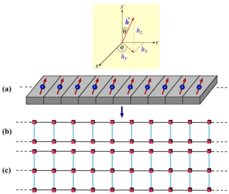
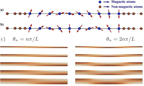
FIG. 1: (Color online) (a) Schematic diagram of a linear netic chain grafted on a substrate (gray blocks). Each mag-netic atom (blue sphere) is subject to a substrate-induced magnetic moment~h = (hx, hy, hz) (red arrow) making an angle θ with the z axis and φ is the azimuthal angle. (b) Schematic representation of a two-strand ladder network with solid lines denoting the hopping elements and cubes repre-senting the effective “sites”. (c) Schematic representation of a three-strand ladder network. The decomposition of~hinto its components is shown in the inset box above the magnetic chain.
the spectra in the respective cases. Section III describes how to engineer the spectral gaps using an appropriate substrate and provides the general criterion for opening up of the spectral gap for arbitrary spins. The discussion is substantiated by a detailed presentation of the density of states (DOS) choosing the spin-1/2 case as example. In section IV we present the results of the transport cal-culations for the spin-1/2 and spin-1 cases. In section V we discuss the idea of having a spin filtering with a cor-related disorder. In section VI we show the robustness of the results by considering a spin-spiral where the sub-strate atoms have their magnetic moments turning se-quentially, in a periodic fashion, mimicking disorder over a length shorter than the period, and in section VII we draw our conclusions. The appendices contain the de-tails of the transport formulation, and further dede-tails are provided in the supplemental material.
II. MODELLING A SPINS CHAIN AS A LADDER OF WIDTH 2S+ 1
In Fig. 1 we propose a model system consisting of a linear array of magnetic atoms grafted on a substrate. The atom at the n-th site has a magnetic moment~hn
[image:3.595.327.552.100.291.2]approximation can be written as
H = X
n
c†nǫn−~hn·Sn(S)
cn+
X
hn,mi
c†ntn,mcm+c†mtn,mcn, (1)
withhn, midenoting nearest neighbors,i.e., m=n±1. Each of the quantitiesc†n,cn,ǫn,tn,m andSn(S) denotes
a multi-component expression according to the spin con-tent, i.e., for the S = 1/2 case, c†n = (c
†
n,↑, c †
n,↓) is the creation operator at thenth site,ǫn= diag (ǫn,↑, ǫn,↓) de-scribes the diagonal on-site potential matrix, andtn,m=
t= diag (t, t) encodes the uniform nearest-neighbor hop-ping integralt along n. The indices ‘↑’, ‘↓’ refer to the spin projections (spin ‘channels’) for the caseS= 1/2.
It is easily appreciated that the dimensions of the ma-trices increase proportionately as one extends the scheme to spin 1, 3/2 or higher values. Consequently, the cre-ation and the annihilcre-ation operators will also have multi-ple components indexed by every single value of the spin projectionmS =−S,−S+ 1,. . .,S−1,S, having a total
of 2S+ 1 values for a general spin-S particle. The term ~hn·Sn(S)=hn,xSn,x(S)+hn,yS(n,yS)+hn,zSn,z(S)describes the
interaction of the spin (S) of the injected particle with the localized on-site magnetic moment~hnat siten. This
term is responsible for spin flipping at the magnetic sites. ForS= 1/2, 1, 3/2,. . ., theSx,Sy,Szdenote the
gener-alized Pauli spin matricesσx,σy, σz expressed in units
of ~S. Spin flip scattering is hence dependent on the
orientation of the magnetic moments~hn in the magnetic
chain with respect to the z axis. Written explicitly for S= 1/2 we have
~hn·Sn(1/2) = hn,xσx+hn,yσy+hn,zσz
=
hncosθn hnsinθne −iφn
hnsinθneiφn −hncosθn
,(2)
with θn and φn denoting polar and azimuthal angles,
respectively.
The time-independent Schr¨odinger equation for the pure spin-1/2 system is written asH|χi =E|χi, where |χi=Pn ψn,↑|n,↑i+ψn,↓|n,↓iis a linear combination of spin-up(↑) and spin-down (↓) Wannier orbitals. Op-eratingH on|χiwe get two equations relating theψn,↑, ψn,↓amplitudes on positionnwith the neighboringn±1 sites,
(E−ǫn,↑+hncosθn)ψn,↑+hnsinθne−iφnψn,↓ =tψn+1,↑+tψn−1,↑, (3a)
(E−ǫn,↓−hncosθn)ψn,↓+hnsinθneiφnψn,↑
=tψn+1,↓+tψn−1,↓. (3b) Eqs. (3a) and (3b) can be expressed in compact form as matrix equation of the form,
(E1−ǫ˜n)ψn=tψn+1+tψn−1, (4)
where
˜
ǫn=
ǫn,↑−hncosθn −hnsinθne −iφn
−hnsinθneiφn ǫn,↓+hncosθn
, (5)
and ψn = (ψn,↑, ψn,↓). We draw the attention of the reader to the equivalence of Eq. (3) to the difference equations for a spinless electron in a two-strand ladder network, as depicted in Fig. 1(b) with an effective on-site potential ǫn,↑−hncosθn, and ǫn,↓ +hncosθn for
the ‘upper’ strand (identified with↑component) and the ‘lower’ strand (identified with↓component) respectively. The amplitude of the hopping integral along each arm of the ladder ist, whilehnsinθnexp(iφn) plays the role of
inter-strandhopping integral along the n-th strand [34]. Similarly, for spinS= 1 particles, we have 2S+ 1 = 3 coupled equations analogous to Eq. (3), namely,
[E−(ǫn,1−hncosθn)]ψn,1+√1
2hnsinθne −iφn
ψn,0=tψn+1,1+tψn−1,1, (6a)
[E−ǫn,0]ψn,0+ 1 √
2hnsinθne
iφn
ψn,1+ 1 √
2hnsinθne −iφn
ψn,−1=tψn+1,0+tψn−1,0, (6b)
[E−(ǫn,−1+hncosθn)]ψn,−1+ 1 √
2hnsinθne
iφnψ
n,0=tψn+1,−1+tψn−1,−1. (6c)
for the three spin projections, viz., +1, 0 and−1. The 3×3 matrix for the ‘effective’ on-site potential at the
n-th position now reads,
˜
ǫn =
ǫn,1−λn −
1 √
2ξne
−iφn 0
−√1 2ξne
iφn ǫ
n,0 −√1 2ξne
−iφn
0 −√1 2ξne
iφn ǫ
n,−1+λn
(a) (b) (c)
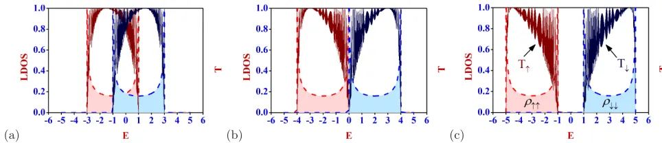
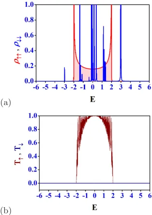
FIG. 2: (Color online) Variation of local density of states (LDOS) and transmission probabilities with energyE as a function ofhfor a fixed value ofθ= 0 for spin-1/2 particles. The light red shaded plot with red envelope is the LDOS for the spin-up (↑) states and the light blue shaded plot with blue envelope is the LDOS for the spin-down (↓) states. The dark red curve represents the transmission characteristics for the spin-up (↑) particles and the dark blue curve is exhibiting the transport for the spin-down (↓) particles. (a) is forh = 1, (b) is for h= 2, and (c) corresponds to h= 3. The lead parameters for the non-magnetic leads areǫL=ǫR= 0 andtLD=tRD=tL=tR= 3.
where λn =hncosθn and ξn =hnsinθn. Clearly, this
can be extended to treat the case of general S, leading to an effective ladder model with 2S+ 1 arms as shown in Fig. 1. The above equations, viz., Eq. (3) and Eq. (6) will now be exploited to engineer the spectral gaps and simulate spin filters, as explained in the subsequent sec-tions.
III. ENGINEERING THE SPECTRAL GAPS
1. Computing the density of states
Its instructive to remind ourselves as to when one can have a gap in the spectrum of such a ladder network in terms of the simplest possible case, where one can set ǫn,↑ = ǫn,↓ = ǫn = ǫ, a constant at all sites n of both
the arms of the ladder, andhn=h. We additionally set
θn=θ andφn= 0. It is easy to understand that, in the
extreme limit of t →0, the spectrum of the two-strand ladder yields sharply localized (pinned) eigenstates at E=ǫ±h. TheDOSwill exhibit twoδ-function spikes at these energy eigenvalues. As the hopping along the arms of the ladder, viz.,t is switched ‘on’, the δfunction like spikes in the DOS spectrum broaden into two subbands, which will finally merge into a single band when h∼t. Therefore, for a given value of the polar angle θ, and a predefined value oft(which sets the scale of energy), the inter-strand hopping h can be tuned to open or close a gap in the energy spectrum.
Mapping back onto the original 1D magnetic chain the above argument clearly shows that one can create gaps in the spectrum or close them, by a judicious engineer-ing of the substrate, that is, the required species of the magnetic atoms providing an appropriate value of the magnetic momenth. This simple argument allows us to gain analytical control over the spectrum and eventually turns out to be crucial in designing a spin filter. In Fig. 2 we show the DOS of a uniform magnetic chain withθ= 0, and φ = 0. The DOS for the ‘up’ and the ‘down’ spin electrons in the magnetic chain withǫ= 0 andt= 1 have
been calculated by evaluating the matrix elements of the Green’s functionG= (E1−H)−1in the Wannier basis |j,↑ (↓)i. The local DOS (same as the average DOS in this case) for the ‘up’ and ‘down’ spin electrons are given by,
ρ↑↑(↓↓)= lim
η→0hj,↑(↓)|G(E+iη)|j,↑(↓)i. (8) Here, ρ↑↑ and ρ↓↓ have been evaluated using a real space decimation renormalization method elaborated elsewhere [38, 39].
2. Substrate-induced opening and closing of spectral gaps
The choice of the strength of the magnetic moment that will make the spectrum gapless is not quite arbitrary. One can, at least for a special relative orientation of the moments at the nearest neighboring sites, work out a pre-scription for this. To appreciate the scheme, let us ob-serve that, even for a site dependent potentialǫnand the
magnetic momenthn, the commutator [˜ǫn,˜ǫn+1] = 0 if
we chooseθn+1−θn=mπ, wherem= 0,±1,±2,±3, .... andφn =φn+1 = 0 or a constant value, irrespective of the values of ǫn or hn. That is, the system may
repre-sent either a ferromagnetic alignment of the moments, or an antiferromagnetic one. Needless to say, the specific case of constant ǫand constant θ falls in this category. In such cases, it is possible to decouple the matrix equa-tion (4) into a set of two independent linear equaequa-tions by making a change of basis, going from ˜ψn toFn, where,
Fn = S−1ψ˜n. S executes a similarity transformation on Eq. (4). The commutation ensures that every ˜ǫn
trix can be diagonalized simultaneously by the same ma-trixS. The concept has previously been used to study the electronic spectrum of disordered and quasiperiodic ladder networks [34–36], and 2D lattices with correlated disorder [37]. The decoupled equations read,
[image:5.595.64.546.96.200.2](a) (b) (c)
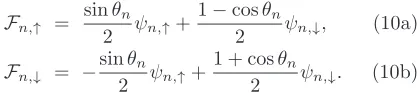
FIG. 3: (Color online) Variation of LDOS and transmission probabilities with energyE as a function ofhfor a fixed value of θ=π/4 for spin-1/2 particles. The curves with the red dashed line represent the LDOS for the spin-up (↑) states and the curves with the blue dashed line represent the LDOS for the spin-down (↓) states. The dark red curve represents the transmission probability for the spin-up (↑) particles and the dark blue curve is exhibiting the transmission probability for the spin-down (↓) particles. (a) is forh= 1, (b) is forh= 2, and (c) corresponds toh= 3.
and represent the equations for twopseudoparticleswith mixed spin states,
Fn,↑ = sinθn
2 ψn,↑+
1−cosθn
2 ψn,↓, (10a) Fn,↓ = −sinθn
2 ψn,↑+
1 + cosθn
2 ψn,↓. (10b) The subscripts ‘↑’ or ‘↓’ in Fn can be taken to be the
indices for the two decoupled arms of the equivalent two-strand ladder.
Let us again get back to the perfectly ordered case with ǫn=ǫ, andhn=h. The first thing to appreciate is that
each individual equation, viz., Eq. (9a) and Eq. (9b) now represents a perfectly periodic array of atomic like sites with an effective on-site potentialǫ±h, and a constant nearest neighbor hopping integral t. Consequently they offer absolutely continuous energy bands, ranging from ǫ−h−2t to ǫ−h+ 2t corresponding to Eq. (9a), and ǫ+h−2ttoǫ+h+ 2tfor the second decoupled equation Eq. (9b). The energy spectrum for the individual infinite chains can be obtained conventionally by working out the DOS for each of them. The DOS of the actual linear magnetic chain is then obtained through a convolution of these two individual DOS’s. It is simple to compute that the gap between the bands is given by,
∆ = 2h−4t. (11) This immediately leads to acriticalvalue of the strength of the magnetic moment hc = 2t for which the gap will
just close. The result is independent of any arbitrary constant value of the polar angleθ, as long as one ensures that the difference between nearest neighboring values of the angle, viz.,θn+1−θn=mπ(m= 0,±1,±2,±3, ....). The variation of the DOS against energy as a function of h is a generic feature of the magnetic array for any constant value of the polar angleθ. This is evident from Figs. 2 and 3, where we have plotted the local density of states (LDOS) at a site in the infinite chain. For a periodic chain the LDOS is same as the average DOS. It is clear from the figures, how a gradual increase in the value of the magnetic momenth, a gap opens in the spectrum,
going through a sequence of variations shown in each panel, where the values ofρ↑↑ andρ↓↓ complement each other. To be noted that, in all the plots the energyE in the abscissa is taken in units oft.
3. Spectral gaps for largerS
A look at the set of Eq. (6) immediately reveals the equivalence of the magnetic chain in the present case with that of a three-strand ladder as depicted in Fig. 1(c). The effective on-site potential at then-th vertex at every strand is given by ǫn−hncosθn, ǫn and ǫn+hncosθn
respectively, while the role of the inter-strand coupling (hopping integral) between the adjacent strands is played byhnsinθn/√2 (with φn is set equal zero). As before,
one can argue that an appropriate tuning of hn (for a
given value ofθn =θ = constant) should open up gaps
in the spectrum, in the same way as it did in the spin-1/2 case. This is precisely what we see in Fig. 4. We have cho-sen a chain with a constant value of the on-site potential ǫn=ǫ,hn has been fixed to any desired constant value,
andθn =φn= 0. The left, middle and the bottom panels
exhibit the overlap of bands forh= 3, the marginal case where the bands just touch each other forh= 4, and a clear opening of the gaps whenh= 6, respectively. The location of the gaps can be estimated quite easily if one observes that withθ = 0, the strands in the three-arm ladder effectively get decoupled, so that one is left with a set of three independent equations representing three individual ordered chains with on site potentialsǫ−h, ǫ, and ǫ+h respectively. The corresponding ranges of eigenvalues are, [ǫ−h−2t, ǫ−h+ 2t,], [ǫ−2t, ǫ+ 2t], and [ǫ+h−2t, ǫ+h+ 2t]. The gap between these ranges can now be estimated in a straightforward way, and the critical value ofh, for which gaps will open for any spin S can thus be worked out to be,
∆(S)= h
S −4t. (12)
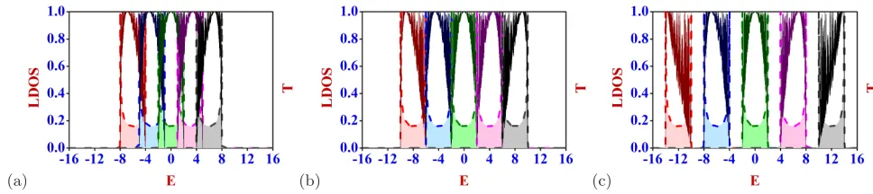
[image:6.595.90.299.317.365.2](a) (b) (c)
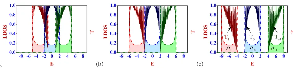
FIG. 4: (Color online) Variation of LDOS and transmission probabilities with energyE as a function ofhfor a fixed value of θ= 0 for spin-1 particles. The light red shaded plot with the dashed red envelope is the LDOS for the spin-1 states, the light blue shaded plot with the blue dashed envelope is the LDOS for the spin-0 states, and the light green shaded plot with the green dashed envelope is the LDOS for the spin-(−1) states. The dark red curve represents the transmission characteristics for the spin-1 particles, the dark blue curve is for the spin-0 particles, and the dark green curve stands for the spin-(−1) particles. (a) is forh= 3, (b) is forh= 4, and (c) corresponds toh= 6. The lead parameters for the non-magnetic leads areǫL=ǫR= 0 andtLD=tRD=tL=tR= 4.
corresponding to the different components of any higher spin. The results for spin 3/2 and spin 2 are shown in the supplemental material [40]. The basic mechanism of designing spin filters by controlling the value and the orientation of the magnetic moments of magnetic atoms in the chain remains the same as we move on to the higher spin states. For the higher spin states the number of spin channels increases, and we have a whole lot of options as to which spin component we want to make transmitting through the system for a certain energy regime. We need to tune the magnitude of h accordingly to have a spin filtering effect as we climb up to the higher spin states.
IV. TWO-TERMINAL TRANSPORT AND SPIN FILTERING
We now discuss the results of two-terminal transport across the magnetic chain. The detailed formulation of the method is provided in the Appendix. For simplicity, we plot the transmission coefficient in each case in the same figure as the corresponding LDOS. We start with the simple case of spin 1/2 andθ= 0, and choose values ofhsuch that there are (a) overlapping, (b) touching and (c) well-separated subbands. From Fig. 2(a) we see that the DOS of the ‘up’ and the ‘down’ spin states forh= 1 overlap over one third of the range of allowed eigenval-ues. The corresponding transmission spectrum naturally offers a mixed character. There is a partial filtering effect with only ‘up’ spin electrons emerging out of the system in the energy interval−3≤E ≤ −1, while it is the op-posite in its positive counterpart. Withh=hc = 2, the
subbands for the ‘up’ and ‘down’ spin states just touch each other. It is obvious from Fig. 2(b) that only ‘up’ spin electrons get transported in the lower half of the band, i.e., in the range −4 ≤ E ≤ 0, while the ‘down’ spin electrons transmit in the range 0≤E ≤4. With h= 3, the gap is explicit, and the spin filtering effect is clear. In this simple case, there is no ‘spin flip’ effect, and the ‘up’ (‘down’) electrons get transmitted precisely in the
energy intervals in which the respective bands are popu-lated. Forθ=π/4 the situation is more complicated as shown in Fig. 3. Here we see that for the same values of has in Fig. 2, we now always get transport with mixed spin-up and spin-down components, even when there is a well-pronounced gap at shown in Fig. 3(c). Adjusting the value ofθ therefore allows to control the relative ad-mixture of the transported spin states while the choice ofh determines the energy range in which the different transport channels will be open.
The behaviour shown for spin-1/2 persists for spin-1 (and higher spin states [40]) as shown Fig. 4 (a), (b) and (c) for θ = 0. The gap opens at a larger value of h, as compared to the spin-1/2 case and can be easily es-timated from Eq. (12). The DOS corresponding to the three spin components, namely, 1, 0 and−1, exhibit over-lap in the panel (a) forh= 3. The critical value ofh= 4 makes the subbands touch each other at the appropri-ate energy values, while a clean gap opens up ash= 6. Consequently, the two terminal transport exhibits a par-tial filtering in selected energy regimes in panel (a) while there is perfect filtering in (b) and (c). We note in (a) that the partial filtering in transmission exists only be-tween the spin channels (1,0) and (0,−1). The results can be understood intuitively if one recalls that S = 1 is identical to the case of a three strand ladder. Since we are working with nearest neighbor hopping in both the longitudinal and the transverse directions and rigid boundary conditions in the y-direction, the upper arm of the ladder (equivalent to the spin-1 channel) is totally decoupled from the lower arm (the spin-(−1) channel). The central arm, namely, the spin-0 channel is coupled to these two outer arms. The partial filtering is thus caused by contributions coming from theinteracting pair
[image:7.595.74.547.93.203.2](a)
(b)
FIG. 5: (Color online) (a) Densities of states of the decoupled set of equations (13) whenǫn=hn=µcos(πQna) withµ= 1 andQ= (√5 + 1)/2. The red and the blue lines correspond to the Eq. (13a) and Eq. (13b) respectively. (b) The zero transmission for the ‘down’ spins reflect the ‘critical’ character of the wavefunctions obtained from Eq. (13b), and the high transmission of the ‘up’ spins reveal the extended nature of the wavefunctions obtained from Eq. (13a), and represents a perfect spin filter. We have sett= 1, and energy is measured in units oft. The lattice constanta= 1.
V. SPIN FILTERING WITH CORRELATED DISORDER
A perfect spin filter can be designed even without setting constant values for the on-site potentials and the substrate magnetic moments, and without bother-ing about engineerbother-ing gaps in the energy spectrum. This can be achieved by introducing correlations between the numerical values of ǫn,↑ =ǫn,↓=ǫn and the magnitude
of the substrate momentshn. We demonstrate a special
situation in Fig. 5. For simplicity, but without sacrific-ing the central spirit, we assign an Aubry-Andre varia-tion [41] in the on-site potential, viz., ǫn =µcos(πQna)
withQ= (√5 + 1)/2. This distribution of the on-site po-tential leads to extended, critical or localized eigenstates forµ <2t,µ= 2tandµ >2t respectively [41]. The dis-tribution of the magnetic moments hn are chosen to be
equal toǫn. In addition, we setθn = 0. With the choice
ofθn= 0, andǫn,↑=ǫn,↓=ǫn, the set of equations (3a)
and (3b) map into the following set of equations, (E−ǫn+hn)ψn,↑=tψn+1,↑+tψn−1,↑, (13a)
(E−ǫn−hn)ψn,↓=tψn+1,↓+tψn−1,↓. (13b) With ǫn = hn, the ‘effective’ on-site potential in
Eq. (13b) is equal to 2µcos(πQna), and a selection of µ= 1 makes the eigenstates corresponding to Eq. (13b)
critical. Eq. (13a), with ǫn = hn, now represents a
perfectly ordered chain with its spectrum ranging from E = −2t to E = 2t. The densities of states and cor-responding transport are shown in Fig. 5. In panel (a), the densities of states for the two decoupled channels are shown. TheDOS for the original system is obtained by convolution of these two, but will definitely encompass the same energy regimes. The ‘up’ spins now have an ab-solutely continuousDOSshown by the red shaded curve, ranging between [−2t,2t]. The critical eigenstates for the ‘down’ spins are shown by the blue lines. As critical and extended states can not coexist at the same energy, the central part of the spectrum will remain extended in the final, convolvedDOS. The outer peaks however, will be there.
The corresponding transport characteristics are repre-sented in panel (b). The total ‘down’ spin transport is naturally blocked, and we now have a clear case of spin filtering even with correlated, but adeterministic disor-der, as is evident from the high transmission of ‘up’ spin states between [−2t,2t]. It can be easily understood that, with a different choice of correlation betweenǫn andhn
(say, ǫn = −hn), we can easily make the ‘down’ spin
channel to be perfectly conducting, and the ‘up’ spins to be completely blocked. As we go to the higher spin cases, the same trick can be used to make one of the spin channels to be perfectly conducting and the rest to be completely blocked. Obviously we need to have different correlations betweenǫn andhn for different cases as we
move along the higher spin ladder.
It is obvious that we need not stick to the case of de-terministic disorder only. If we choose bothǫn andhn in
a random yet in correlated way, such thatǫn−hn = Λ
remains a constant, i.e., n-independent, then Eq. (9a) yields an absolutely continuous spectrum in the range Λ−2t≤ E ≤Λ + 2t. This will be true even when the constant value of the polar angleθ 6= 0. All eigenstates in this energy range have to be of extended Bloch func-tions. On the other hand, even with this choice, Eq. (9b) represents a randomly disordered chain of scatterers for which the pseudoparticle states with mixed spin status will be Anderson localized. The system will then open up a transmitting channel for suchmixed spin statesonly in the window Λ−2t≤E≤Λ + 2t, while it will remain opaque to all incoming electrons, irrespective of their spin states, in the energy regime beyond these limits [46].
The above argument holds, and the scenario may even become richer, as probes with higher spin states are in-cident on the magnetic substrate. For a total spin S, with the same restriction on the polar angleθn, and the
azimuthal angleφn being set equal to zero, the matrix
equation Eq. (4) decouples into a set of 2S+ 1 indepen-dent equations, each representing a pseudoparticle with a mixed spin state (now much more complicated). One can then introduce a correlation betweenǫn andhn, keeping
[image:8.595.97.254.102.323.2]be-like distributions on either side of the central continuum. Considering the overall charge transport, such cases may even give rise to the possibility of a metal-insulator tran-sition. The situation is to be contrasted with the case of a real multiple stranded ladder network [37] remember-ing that, here we have just a sremember-ingle magnetic chain. It is the spin state of the incoming particle that will decide whether such a simple quantum device will show up any reentrant behavior in charge transport or not.
VI. A SPIN SPIRAL: SIMULATING ‘LOCAL’ DISORDER
In this section we extend the concepts developed in the earlier sections to a patterned magnetic chain mimicking a spin spiral [42] in one dimension. Then-th atomic site
(c) θn=nπ/L θn= 2nπ/L
FIG. 6: (Color online) Schematic diagram of linear array of magnetic atoms (blue spheres) with magnetic moment vectors ~h(red arrows) forming spiral configurations for (a)θn=nπ/L and (b) 2nπ/L. The system is connected between two non-magnetic semi-infinite leads (brown spheres). The horizontal lines are guides to the eye only. (c) Color representation of the on-site potentialhcosθnof spiral configurations atL= 72 for (left)θn=nπ/Land (right) 2nπ/Lcorresponding toS= 1/2, 1,. . ., 5/2 from top to bottom. Dark colors correspond to large values.
now has its magnetic moment tilted with respect to the global magnetization axis (the z-axis) by an angle θn.
As we neglect any spin-orbit interaction in this work, the spin and the position spaces are decoupled, and the relative orientation of the neighboring spin becomes im-portant in respect of the transport and other physical properties. Here we stick to a periodic variation of the spiral, though the period can be quite arbitrary. The configuration is schematically depicted in Fig. 6 and can
for a spiral patch with length restricted to less than a period or its integral multiple, may show up some char-acter expected for a real disordered magnetic chain, and test the robustness of the results obtained earlier.
We follow the same RSRG decimation scheme used earlier to study the LDOS at a bulk site forθn =nπ/L
and θn = nπ/(L/2). Even when the strength of the
magnetic momenthis set to be same at every magnetic site, the variation inθn naturally leads to variations in
the values ofhcosθn and hsinθn. This implies that we
have a magnetic chain of atoms with a (deterministic) fluctuation both in the effective on site potential, viz., ǫ±hcosθn and the ‘coupling’hsinθn between the ‘up’
and the ‘down’ spin channels. Mapping into the effective multi-strand ladder network, we have a case of a ladder where the ‘rungs’ are associated with varying hopping integrals, simulating a kind of deformation, and where, at the same time the vertices are occupied by atomic sites with sequentially changing on-site potentials, see Fig. 6(c).
In Fig. 7 we show the variation of the LDOS and cor-responding transmission spectrum for a spin-1/2 spiral configuration. The periods of the spiral configurations are chosen to be 600 and 300 corresponding to Fig. 7(a), (b) and (c), (d) respectively. We have seth= 2 through-out and have takenL= 300. The energy bands for the ‘up’ and the ‘down’ spin channels touch each other at thishas in Figs. 2 and 3. However, in contradistinction to these previous results, we now observe a spin-flipped transmission in Fig. 7(a), and (b). This can be under-stood if we recall that the ‘effective’ on-site potentials for the ‘up’ and the ‘down’ spin electrons turn out to be −hcos(nπ/L) andhcos(nπ/L) respectively. The period of variation inθn is 2L. Thus, for a system size equal to
half the period, the incoming ‘up’ particle traverses the potential landscape uphill, as shown in Fig. 6(c). The transport of ‘up’ spin electrons thus experiences resis-tance in traversing the system, and is eventually blocked over the energy range−4 < E <0, though ρ↑↑ is finite here. On the other hand, the ‘down’ spin electrons effec-tively movedownhillon the potential landscape, and are transmitted in the same energy range. The complemen-tary picture is visible in Fig. 7(b). The specific choice of the polar angleθn =nπ/Lthus makes the L-atom long
system aspin flipper.
The argument laid down here helps us understand the remaining two figures viz., Fig. 7 (c) and (d). We have now selected θn = nπ/(L/2) and a system of length L
[image:9.595.56.299.391.536.2]fa-(a) (b)
(c) (d)
FIG. 7: (Color online) Plot of LDOS and transmission probabilities for spin-1/2 particles for spiral configurations of the magnetic moments in the magnetic chain system. The figures in the top panel [(a) and (b)] is for a variation of the angle θn =nπ/L, and the figures in the bottom panel [(c) and (d)] correspond to an angle variationθn=nπ/(L/2) with L= 300. We have seth= 2 for all the magnetic sites in the chain.
voring the ‘up’ spin transport. The case is similar for the ‘down’ spin states, but in the complementary range of the energy. We do not have a spin flipper anymore. The results for higher spin S are presented in the sup-plement [40]. There will bemS ‘spin channels’, e.g., for
S = 1, the central channel, corresponding to the spin projectionmS = 0, turns out to be always transmitting,
while the channels corresponding to mS = ±1 exhibit
spin-flipped transport forθn =nπ/L. The spin flipping
character is lost if the system size includes a full period of variation in the polar angleθn, just as it was for the
spin-1/2 case. We have also checked that a variation of the simple harmonic spiral variation presented here, using e.g. θn ∝ √n or n2, does not alter the overall
spin-flipping presented here.
VII. CONCLUSION
In conclusion, we have presented a simple one dimen-sional chain of magnetic atoms which can act as spin filter or spin flipper for particles with arbitrary spins. The central idea depends crucially on a mapping of the problem for a spin-S particle into that of a 2S+ 1 strand ladder network. The magnetic moment of the substrate atoms turns out to be equivalent to the ‘inter-strand’ tun-nel hopping integral, which needs to be tailored to open up gaps in theDOS. This is shown to lead to the desired spin filtering effect. The analysis has been carried out for a wide variety of spins, going well beyond the standard spin-1/2 case. Higher spins are obtainable in appropriate atomic gases. The present work presents a unified model which can, in principle, through an appropriate substrate engineering, filter out arbitrarily large spin components,
treating fermions and bosons on the same footing.
Talking about the experimental aspects of the work, the model system proposed by us can actually be realised now a days experimentally as well. With the present day advanced technologies people can image and manipulate the spin direction of individual magnetic atoms [43] to grow nanomagnets where exchange-coupled atomic mag-netic moments form an array. Such tailor-made nano-magnets posses a rich variety of magnetic properties and can be explored as constituents of nanospintronics tech-nologies [44]. So the model magnetic chains proposed by us are not far from reality. The concept of spin transport for higher spin states can be realised in atomic gases, and may lead to some exciting new generation spin-based de-vices. The idea of filtering out one of the spin components for a certain energy regime can have useful application in spin-based logic gates [45].
Acknowledgments
[image:10.595.147.465.98.305.2]
ψn+1,↑ ψn+1,↓ ψn,↑ ψn,↓
=
(E−ǫn,↑+hncosθn)
t
hnsinθne−iφn
t −1 0
hnsinθneiφn
t
(E−ǫn,↓−hncosθn)
t 0 −1
1 0 0 0
0 1 0 0
| {z }
Pn
ψn,↑ ψn,↓ ψn−1,↑ ψn−1,↓
. (A.1)
wherePnis thetransfer matrix for then-th site. We have a system (magnetic chain) withN number of magnetic sites connected between two semi-infinite non-magnetic leads. So the matrix equation connecting the wave functions of the lead-system-lead bridge is given by,
ψN+2,↑ ψN+2,↓ ψN+1,↑ ψN+1,↓
=MR·P ·ML | {z }
M
ψ0,↑ ψ0,↓ ψ−1,↑ ψ−1,↓
. (A.2)
where ML is the transfer matrix for the left lead, MR is the transfer matrix for the right lead,P =Q1n=NPn, and M is the total transfer matrix for the lead-system-lead bridge.
2. Evaluation ofML
We have set ǫL = ǫ0 for the all the sites in the left
lead. The difference equation connecting the wave func-tion amplitude of the 0-th site with that of the 1-th and −1-th sites is,
(E−ǫ0)ψ0=tLDψ1+tLψ−1. (A.3)
In the lead, according to the tight-binding model, we have ψn = Aeikna and ψ0 = eiγLψ−1, where γL = ka
and E = ǫ0+ 2tLcosγL. Consequently we find ψ1 =
tLeiγL/tLDψ0. In TMM form, this gives
ψ1,↑ ψ1,↓ ψ0,↑ ψ0,↓
= tL
tLDe
iγL 0 0 0
0 tL tLD
eiγL 0 0
0 0 eiγL 0
0 0 0 eiγL
| {z }
ML
ψ0,↑ ψ0,↓ ψ−1,↑ ψ−1,↓
. (A.4)
3. Evaluation ofMR
We set ǫR = ǫ0 for the all the sites in the right lead.
The difference equation connecting the wave function am-plitude of the (N+ 1)-th site with that of the (N+ 2)-th andN-th sites is,
(E−ǫ0)ψN+1=tRψN+2+tRDψN, (A.5)
whereψN+2=Aeik(N+2)a;ψN+2=eiγRψN+1, andγR=
ka and E = ǫ0+ 2tRcosγR. Consequently, ψN+1 = tRDeiγR/tRψN and
ψN+2,↑ ψN+2,↓ ψN+1,↑ ψN+1,↓
=
eiγR 0 0 0
0 eiγR 0 0
0 0 tRD tR
eiγR 0
0 0 0 tRD tR
eiγR
| {z }
MR
ψN+1,↑ ψN+1,↓ ψN,↑ ψN,↓
a. An incoming spin up(↑)
If the incoming particle to the left electrode (lead) has a spin-up (↑) projection then the wavefunction ampli-tudes in Eq. (A.2) can be written as, ψ−1,↑ =e−iγL + R↑↑eiγL, ψ−1,↓ = R↑↓eiγL, ψ0,↑ = 1 + R↑↑, ψ0,↓ = R↑↓, ψN+2,↑ = T↑↑ei(N+2)γR, ψN+2,↓ = T↑↓ei(N+2)γR, ψN+1,↑ = T↑↑ei(N+1)γR, ψN+1,↓ = T↑↓ei(N+1)γR, where R↑↑(↑↓) and T↑↑(↑↓) are the amplitudes of the reflected and transmitted electron wavefunctions with spin-up (↑) projection, which remain in spin-up (↑) state (or, flip to spin-down (↓) state) after passing through the system. If we put the above values of the wavefunction amplitudes in Eq. (A.2) then we will have
T↑↑ei(N+2)γR
T↑↓ei(N+2)γR
T↑↑ei(N+1)γR T↑↓ei(N+1)γR
=M
1 +R↑↑ R↑↓ e−iγL+
R↑↑eiγL R↑↓eiγL
. (A.7)
We solve Eq. (A.7) forT↑↑andT↑↓ and obtain the trans-mission probabilities as
T↑↑ =tRsinγR tLsinγL
T↑↑
2, T↑↓= tRsinγR tLsinγL
T↑↓
2. (A.8)
The total transmission probability for a spin-up (↑) par-ticle is given by,
T↑=T↑↑+T↑↓. (A.9)
b. An incoming spin down(↓)
If the incoming particle to the left electrode (lead) has a spin down (↓) projection then ψ−1,↑ = R↓↑eiγL,
ψ−1,↓ = e−iγL +R↓↓eiγL, ψ0,↑ = R↓↑, ψ0,↓ = 1 + R↓↓, ψN+2,↑ = T↓↑ei(N+2)γR, ψN+2,↓ = T↓↓ei(N+2)γR, ψN+1,↑ = T↓↑ei(N+1)γR, ψN+1,↓ = T↓↓ei(N+1)γR, where R↓↓(↓↑) and T↓↓(↓↑) are the amplitudes of the reflected and transmitted electron wavefunctions with spin-down (↓) projection, which remain in spin-down (↓) state (or, flip to spin-up (↑) state) after passing through the sys-tem. As before, we find
T↓↑ei(N+2)γR
T↓↓ei(N+2)γR T↓↑ei(N+1)γR T↓↓ei(N+1)γR
=M R↓↑ 1 +R↓↓ R↓↑eiγL e−iγL+R↓↓eiγL
. (A.10)
and solve Eq. (A.10) forT↓↓ and T↓↑. The transmission probabilities are now
T↓↓=
tRsinγR
tLsinγL
T↓↓2, T↓↑=
tRsinγR
tLsinγL
T↓↑2, (A.11) with total transmission probability for a spin-down (↓) particle
T↓=T↓↓+T↓↑. (A.12)
4. An example for higher spin cases: spin1
Proceeding in the same way as in the spin-1/2 case, we obtain the following forms of the trans-fer matrices for the left and right leads as, ML = eiγLdiag (t
L/tLD, tL/tLD, tL/tLD,1,1,1) and MR = eiγRdiag (1,1,1, t
R/tRD, tR/tRD, tR/tRD). The transfer
matrix for spin-1 particles at then-th site reads as,
Pn=
(E−ǫn,1+hncosθn)
t
hnsinθne−iφn
√
2t 0 −1 0 0
hnsinθneiφn
√ 2t
(E−ǫn,0)
t
hnsinθne−iφn
√
2t 0 −1 0
0 hnsinθne
iφn
√ 2t
(E−ǫn,−1−hncosθn)
t 0 0 −1
1 0 0 0 0 0
0 1 0 0 0 0
0 0 1 0 0 0
. (A.13)
Similar to the spin-1/2 particles, we obtain the transmis-sion probabilities for the spin-1 particles as,
Tσσ′ =
tRsinγR
tLsinγL
Tσσ′
2, (A.14)
the transport characteristics for particles with any ar-bitrary spin. For spin S = 1/2 in (A.1) and for S = 1 in (A.13), the on-site magnetic strength coeffi-cients ∝ cosθn are 1, −1 and 1, 0, −1, respectively.
1/√5,√8/5,3/5,√8/5,1/√5. These coefficients, for the cosθn terms, are used in Fig. 6(c).
[1] G. A. Prinz, Phys. Today 48, 58 (1995); Science 282, 1660 (1998).
[2] S. A. Wolf, D. D. Awschalom, R. A. Buhrman, J. M. Daughton, S. von Moln´ar, M. L. Roukes, A. Y. Chtchekanova, and D. M. Treger, Science 294, 1488 (2001).
[3] M. Julliere, Phys. Lett. A54, 225 (1975).
[4] J. S. Moodera, L. R. Kinder, T. M. Wong, and R. Meser-vey, Phys. Rev. Lett.74, 3273 (1995).
[5] M. N. Baibich, J. M. Broto, A. Fert, F. N. Van Dau, F. Petroff, P. Etienne, G. Creuzet, A. Friederich, and J. Chazelas, Phys. Rev. Lett.61, 2472 (1988).
[6] D. Goldhaber-Gordon, H. Shtrikman, D. Mahalu, D. Abusch-Magder, U. Meirav, and M. A. Kastner, Nature (London)391, 156 (1998).
[7] S. M. Cronenwett, T. H. Oosterkamp, and L. P. Kouwen-hoven, Science281, 540 (1998).
[8] H. Yu and J.-Q. Liang, Phys. Rev. B72, 075351 (2005). [9] L. P. Rokhinson, V. Larkina, Y. B. Lyanda-Geller, L. N. Pfeiffer, and K. W. West, Phys. Rev. Lett.93, 146601 (2004).
[10] N. Tombros, C. Jozsa, M. Popinciuc, H. T. Jonkman, and B. J. Van Wees, Nature448, 571 (2007).
[11] S. K. Watson, R. M. Potok, C. M. Markus, and V. Uman-sky, Phys. Rev. Lett.91, 258301 (2003).
[12] E. R. Mucciolo, C. Chamon, and C. M. Marcus, Phys. Rev. Lett.89, 146802 (2002).
[13] V. Rodrigues, J. Bettini, P. C. Silva, and D. Ugarte, Phys. Rev. Lett.91, 096801 (2003).
[14] J. E. Birkholz and V. Meden, Phys. Rev. B79, 085420 (2009).
[15] R. P. Andres, T. Bein, M. Dorogi, S. Feng, J. I. Hender-son, C. P. Kubiak, W. Mahoney, R. G. Osifchin, and R. Reifenberger, Science272, 1323 (1996).
[16] N. Sergueev, Q.-feng Sun, H. Guo, B. G. Wang, and J. Wang, Phys. Rev. B65, 165303 (2002).
[17] H.-F. L¨u, S.-S. Ke, X.-T. Zu, and H.-W. Zhang, J. Appl. Phys.109, 054305 (2011).
[18] R. Wang and J.-Q. Liang, Phys. Rev. B 74, 144302 (2006).
[19] A. A. Shokri and M. Mardaani, Solid State Comm.137, 53 (2006).
[20] A. A. Shokri, M. Mardaani, and K. Esfarjani, Physica E 27, 325 (2005).
[21] M. Mardaani and A. A. Shokri, Chem. Phys.324, 541 (2006).
[22] M. Dey, S. K. Maiti, and S. N. Karmakar, Phys. Lett. A
374, 1522 (2010).
[23] M. Dey, S. K. Maiti, and S. N. Karmakar, Eur. Phys. J. B80, 105 (2011).
[24] M. Dey, S. K. Maiti, and S. N. Karmakar, J. Comput. and Theo. Nanosc.8, 253 (2011).
[25] C. N´u˜nez, F. Dom´ınguez-Adame, P. A. Orellana, L. Ros-ales, and R. A. R¨omer, 2D Mater.3, 025006 (2016). [26] C. Betthausen, T. Dollinger, H. Saarikoski, V. Kolkovsky,
G. Karczewski, T. Wojtowicz, K. Richter, and D. Weiss, Science337, 324 (2012).
[27] H. Saarikoski, T. Dollinger, and K. Richter, Phys. Rev. B86, 165407 (2012).
[28] P. W´ojcik, J. Adamowski, M. Wooszyn, and B. J. Spisak, Semicond. Sci. Technol.30, 065007 (2015).
[29] J. L. Pichard and G. Sarma, J. Phys. Colloques42, C4-37 (1981).
[30] A. MacKinnon and B. Kramer, Z. Phys. B53, 1 (1983). [31] Y. Jiang, X. Guan, J. Cao, and H.-Q. Lin, Nucl. Phys. B
895, 206 (2015).
[32] G. Paganoet al., Nat. Phys.10, 198 (2014).
[33] M. Fattori, T. Koch, S. Goetz, A. Griesmaier, S. Hensler, J. Stuhler, and T. Pfau, Nat. Phys.2, 765 (2006). [34] S. Sil, S. K. Maiti, and A. Chakrabarti, Phys. Rev. Lett.
101, 076803 (2008).
[35] S. Sil, S. K. Maiti, and A. Chakrabarti, Phys. Rev. B78, 113103 (2008).
[36] B. Pal and A. Chakrabarti, Physica E60, 188 (2014). [37] A. Rodriguez, A. Chakrabarti, and R. A. R¨omer, Phys.
Rev. B86, 085119 (2012).
[38] A. Chakrabarti, S. N. Karmakar, and R. K. Moitra, Mod. Phys. Lett. B4, 795 (1990).
[39] M. Leadbeater, R. A. R¨omer, and M. Schreiber, Eur. Phys. J. B8, 643 (1999).
[40] See Supplemental Material at [URL will be inserted by publisher] for higher spin results.
[41] S. Aubry and G. Andr´e, Ann. Israel Phys. Soc.3, 133 (1980).
[42] J. Enkovaara, A. Ayuela, J. Jalkanen, L. Nordstr¨om, and R. M. Nieminen, Phys. Rev. B67, 054417 (2003). [43] D. Serrate, P. Ferriani, Y. Yoshida, S.-W. Hla, M.
Men-zel, K. von Bergmann, S. Heinze, A. Kubetzka, and R. Wiesendanger, Nat. Nanotechnol.5, 350 (2010). [44] A. A. Khajetoorians, J. Wiebe, B. Chilian, S. Lounis, S.
Bl¨ugel, and R. Wiesendanger, Nat. Phys.8, 497 (2012). [45] A. A. Khajetoorians, J. Wiebe, B. Chilian, and R.
Wiesendanger, Science332, 1162 (2011).
choos-ing ǫn+hn = Λ. Then Eq. (9b) yields an absolutely continuous spectrum and Eq. (9a) represents a randomly disordered chain. Of course, the pertinent issue in this case is not filtering out a particular spin state. Instead,
for higher spin states – both for the constant values of the polar angleθas well as for a ‘spiral’ configuration in
θ. These results are complementary to the results dis-cussed in the main paper. The methods and mathemat-ical framework we have used to obtain these results are already discussed in the main paper.
I. CONSTANT POLAR ANGLEθ
In this section we present the results for constant polar angle θ. In Fig. S1 we show the local density of states (LDOS) and the corresponding two terminal transmis-sion coefficient for a fixedθ=π/4 and for different values of the strength of the magnetic momenth. This figure is the counter part of Fig. 4 in the main text for non-zero value of θ. In Fig. S2 and Fig. S3 we have exhibited a similar analysis corresponding to the spin-3/2 and spin-2 cases for θ = 0. These two figures are complementary to the Figs. 2 and 4 given in the main article but now for higher spin states. Here we have a larger number of bands corresponding to different spin channels as the number of spin components has increased. The central idea remains the same as discussed in the main paper for
II. SPIRAL CASES
In Fig. S4, and Fig. S5 we show results for the LDOS and transmission characteristics corresponding to spins
(a) (b) (c)
FIG. S1: (Color online) Variation of LDOS and transmission probabilities with energyEas a function ofhfor a fixed value of
θ=π/4 for spin-1 particles. The curves with the red dashed line represent the LDOS for the spin-1 states, the curves with the
blue dashed line represent the LDOS for the spin-0 states, and the the curves with the green dashed line represent the LDOS
for the spin-(−1) states. The dark red curve represents the transmission probability for the spin-1 particles, dark blue curve
represents the transmission probability for the spin-0 particles,the dark green curve is exhibiting the transmission probability
for the spin-(−1) particles. (a) is for h= 3, (b) is for h= 4, and (c) corresponds to h = 6. The lead parameters for the
non-magnetic leads areǫL=ǫR= 0 andtLD=tRD=tL=tR= 4.
(a) (b) (c)
FIG. S2: (Color online) Variation of LDOS and transmission probabilities with energyEas a function ofhfor a fixed value of
θ= 0 for spin-3/2 particles. The light red shaded plot with the dashed red envelope is the LDOS for the spin-3/2 states, the
light blue shaded plot with the blue dashed envelope is the LDOS for the spin-1/2 states, the light green shaded plot with the
green dashed envelope is the LDOS for the spin-(−1/2) states, and the light magenta shaded plot with the magenta dashed
envelope is the LDOS for the spin-(−3/2) states. The dark red curve represents the transmission characteristics for the spin-3/2
particles, the dark blue curve is for the spin-1/2 particles, the dark green curve is for the spin-(−1/2) particles, and the dark
magenta curve is for the spin-(−3/2) particles. (a) is for h= 4.5, (b) is for h= 6, and (c) corresponds toh= 9. The lead
parameters for the non-magnetic leads areǫL=ǫR= 0 andtLD=tRD=tL=tR= 6.
(a) (b) (c)
FIG. S3: (Color online) Variation of LDOS and transmission probabilities with energyE as a function ofhfor a fixed value
ofθ = 0 for spin-2 particles. The light red shaded plot with the dashed red envelope is the LDOS for the spin-2 states, the
light blue shaded plot with the blue dashed envelope is the LDOS for the spin-1 states, the light green shaded plot with the green dashed envelope is the LDOS for the spin-0 states, the light magenta shaded plot with the magenta dashed envelope is
the LDOS for the spin-(−1) states, and the light gray shaded plot with the dark gray dashed envelope is the LDOS for the
spin-(−2) states. The dark red curve represents the transmission characteristics for the spin-2 particles, the dark blue curve is
for the spin-1 particles, the dark green curve is for the spin-0 particles, the dark magenta curve is for the spin-(−1) particles,
and the black curve is for spin-(−2) particles. (a) is for h = 6, (b) is for h= 8, and (c) corresponds to h = 12. The lead
[image:16.595.66.547.94.202.2] [image:16.595.65.548.316.423.2] [image:16.595.63.547.545.653.2](a) (b) (c)
(d) (e) (f)
FIG. S4: (Color online) Plot of LDOS and transmission probabilities for spin-1 particles for spiral configurations of the magnetic
moments in the magnetic chain system. The figures in the top panel [(a), (b) and (c)] is for a variation of the angleθn=nπ/L,
and the figures in the bottom panel [(d), (e) and (f)] correspond to an angle variationθn=nπ/(L/2) withL= 300. We have
seth= 4 for all the magnetic sites in the chain.
(a) (b) (c) (d)
(e) (f) (g) (h)
FIG. S5: (Color online) Plot of LDOS and transmission probabilities for spin-3/2 particles for spiral configurations of the
magnetic moments in the magnetic chain system. The figures in the top panel [(a), (b), (c) and (d)] is for a variation of the
angle θn=nπ/L, and the figures in the bottom panel [(e), (f), (g) and (h)] correspond to an angle variationθn=nπ/(L/2)
[image:17.595.71.546.94.304.2] [image:17.595.66.555.493.651.2]