by Eddie C. Davis
A dissertation
submitted in partial fulfillment of the requirements for the degree of
Doctor of Philosophy in Computing Boise State University
DEFENSE COMMITTEE AND FINAL READING APPROVALS
of the dissertation submitted by
Eddie C. Davis
Dissertation Title: Polyhedral+Dataflow Graphs Date of Final Oral Examination: 6th December 2019
The following individuals read and discussed the dissertation submitted by student Eddie C. Davis, and they evaluated the presentation and response to questions during the final oral examination. They found that the student passed the final oral examination.
Catherine RM. Olschanowsky, Ph.D. Chair, Supervisory Committee Elena Sherman, Ph.D. Member, Supervisory Committee Steven Cutchin, Ph.D. Member, Supervisory Committee Donna Calhoun, Ph.D. Member, Supervisory Committee
The final reading approval of the dissertation was granted by Catherine RM. Olschanowsky, Ph.D., Chair of the Supervisory Committee. The dissertation was approved by the Graduate College.
The author wishes to express gratitude to his advisor, Catherine Olschanowsky, for her unwavering patience, encouragement, and support.
This work has been partially supported by the National Science Foundation under Grant Numbers 1422725, 1563818, and by the U.S. Department of Energy, Office of Science, Advanced Scientific Computing Research Program under Award Number DE-SC-04030, and contract number DE-AC02-05-CH11231. Any opinions, findings, and conclusions or recommendations expressed in this material are those of the author and do not necessarily reflect the views of the Department of Energy.
This research presents an intermediate compiler representation that is de-signed for optimization, and emphasizes the temporary storage requirements and execution schedule of a given computation to guide optimization decisions. The representation is expressed as a dataflow graph that describes computational state-ments and data mappings within the polyhedral compilation model. The targeted applicationsinclude boththe regular and irregular scientific domains.
The intermediate representation can be integrated into existing compiler infras-tructures. A specification language implemented as a domain specific language in C++ describes the graph components and the transformationsthat can be applied. Thevisual representationallows userstoreasonaboutoptimizations. Graphvariants can be translated into source code or other representation. The language, interme-diate representation, and associated transformations have been applied to improve the performance of differential equation solvers, or sparse matrix operations, tensor decomposition, and structured multigrid methods.
ABSTRACT . . . 6 LIST OF TABLES . . . 12 LIST OF FIGURES . . . 13 LIST OF ABBREVIATIONS . . . 18 LIST OF SYMBOLS . . . 21 1 Introduction . . . 1 1.1 Contributions . . . 4 1.2 Dissertation Structure . . . 6 2 Background . . . 7 2.1 Compiler Optimizations . . . 7 2.2 Polyhedral Model . . . 10 2.3 Dataflow Languages . . . 14 2.4 Memory Optimizations . . . 15
2.5 Target Computational Patterns . . . 15
2.5.1 Iterative Methods . . . 16
2.5.2 Gradient Methods . . . 17
2.5.3 Finite Difference and Volume Methods . . . 19 vii
2.5.5 Tensor Decomposition . . . 23
2.6 Sparse Matrix Formats . . . 25
3 Polyhedral+Dataflow Graph Intermediate Representation . . . 30
3.1 Polyhedral+Dataflow Graphs . . . 31 3.1.1 Graph Components . . . 32 3.1.2 MiniFluxDiv Benchmark . . . 35 3.1.3 Execution Schedule . . . 37 3.1.4 Cost Model . . . 37 3.2 Graph Operations . . . 40 3.2.1 rescheduleOperation . . . 40 3.2.2 fuse Operations . . . 40 3.2.3 Overlapped Tiling . . . 42
3.2.4 Mapping Data to Memory . . . 43
3.3 Experimental Evaluation . . . 44
3.3.1 Experimental Setup . . . 46
3.3.2 Benchmark Variants . . . 48
3.3.3 Temporary Storage Reductions . . . 51
3.3.4 Overlapped Tiling Comparison . . . 52
3.3.5 Halide and PolyMage Comparisons . . . 53
3.3.6 AMR-Godunov Solver . . . 53
3.4 Summary . . . 56
4 Polyhedral+Dataflow Specification Language . . . 57
4.1 Polyhedral+Dataflow Language . . . 58
4.1.2 Memory Allocation . . . 63
4.2 Compilation Approach . . . 65
4.2.1 Derivation from Existing Code . . . 65
4.2.2 Graph Generation . . . 65 4.2.3 Code Generation . . . 67 4.2.4 Data Types . . . 68 4.2.5 Data Mapping . . . 69 4.2.6 Limitations . . . 69 4.3 Inspector/Executor Applications . . . 70
4.3.1 Sparse Matrix-Vector Multiplication . . . 70
4.3.2 Matricized Tensor Times Khatri-Rao Product . . . 75
4.4 Experimental Evaluation . . . 79
4.4.1 Target Architecture . . . 79
4.4.2 CSR to BCSR for Sparse Matrices . . . 79
4.4.3 COO to CSF for Sparse Tensors . . . 80
4.5 Summary . . . 81
5 Structured Grid Solver Integration . . . 85
5.1 Background . . . 86
5.1.1 Chombo and AMR . . . 86
5.1.2 Euler Equations . . . 87
5.2 Proto Overview . . . 88
5.2.1 Euler in Proto . . . 89
5.3 Compiler Approach . . . 91
5.3.2 Mapping Proto to Polyhedral+Dataflow IR . . . 91
5.3.3 Performance Modeling . . . 93
5.3.4 Shift and Fuse Algorithm . . . 95
5.4 Code Generation . . . 99
5.5 Experimental Evaluation . . . 99
5.5.1 Experimental Setup . . . 100
5.5.2 Code Variants . . . 101
5.6 Summary . . . 103
6 Irregular Algorithm Implementations . . . 105
6.1 Conjugate Gradient . . . 105 6.1.1 Executor Definitions . . . 106 6.1.2 Inspector Construction . . . 107 6.1.3 Code Generation . . . 110 6.2 Tensor Decomposition . . . 112 6.2.1 Inspector Construction . . . 114 6.2.2 CP-ALS Implementation . . . 115 6.2.3 Code Generation . . . 117 6.3 Experimental Evaluation . . . 118 6.4 Summary . . . 121 7 Related Work . . . 125 7.1 Programming Languages . . . 125 7.2 Scripting Languages . . . 127 7.3 Intermediate Representations . . . 129 x
7.4.1 Non-affine Transformations . . . 133
7.4.2 Tensor Compilers . . . 133
7.4.3 Visualization Tools . . . 134
7.4.4 Memory Optimizations . . . 134
7.5 Library Based Approaches . . . 135
7.5.1 Adaptive Mesh Refinement . . . 136
7.6 Performance Modeling . . . 137
7.7 Autotuning . . . 138
7.8 Summary . . . 140
8 Conclusions and Future Work . . . 141
8.1 Compiler IR for Loop and Data Transformations . . . 141
8.2 Domain Specific Language . . . 141
8.3 Integration with Existing Application . . . 142
8.4 Algorithms with Sparse Structures . . . 142
8.5 Contributions . . . 143
8.6 Future Directions . . . 144
REFERENCES . . . 146
5.1 Performance model for the three Euler graph variants, indicating the relationship between storage reduction, increased arithmetic intensity, and performance speedup. . . 95
6.1 Summary of matrix formats, expected sizes, mean sizes, and corre-sponding experimental mean speedups on Intel Xeon CPU. . . 120
7.1 Summary of related programming language, compiler, and library-based technologies for algorithmic representation and optimization. . . . 140
2.1 Process flow of an optimizing compiler with parser (front), optimization passes (middle), code generator, and linker (back-end components). . . 8 2.2 Source code for Newton-Raphson method. . . 16 2.3 Cell fluxes across surface faces of control volume. . . 20 2.4 Source code for 2D smoothing stencils. . . 22 2.5 Source code for Matricized Tensor Times Khatri-Rhao product for
fourth order tensor. . . 25 2.6 CP-ALS decomposition algorithm with R components for Nth order
tensor,X. . . 26 2.7 Sparse Matrix Formats . . . 28 2.8 Sparse Tensor Formats . . . 29
3.1 Overview of the three code generation phases using loop chain pragmas and the polyhedral+dataflow graph method and associated cost model. 31 3.2 Summary of graph components, including edges, data, statement, and
transformation nodes. . . 33 3.3 A graph representation of the series of loops implementation of the
MiniFluxdiv benchmark. This schedule uses static single assign-ment for all values produced within the represented computation. . . 38 3.4 The set of operations that are defined for dataflow graphs. . . 39
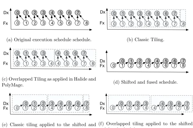
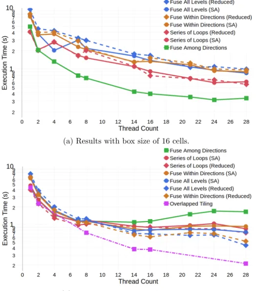
tiling variants. . . 41 3.6 Performance of the MiniFluxdiv benchmark on 28-Core Intel Xeon
E5-2680 CPU for both (a) small (163) and (b) large (1283) boxes. The
y-axis is in log scale. . . 45 3.7 Graph for fuse among directions variant (green line in Figure 3.6). . . 46 3.8 Graph for fuse within directions variant (orange lines in Figure 3.6). . . 47 3.9 Graph for fuse all levels variant (blue lines in Figure 3.6). . . 48 3.10 The execution time for schedules with storage mapping optimizations
are significantly faster for most schedules. The original times are represented by the light gray bars, and the dark bars indicate the reduced times. . . 50 3.11 Overlapped tiling comparison of the two techniques applied to the
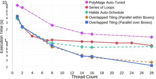
MiniFluxDiv benchmark, including the original series of loops im-plementation as a reference. The x-axis is tiling method within box size and thread count. The y-axis is in log scale. . . 51 3.12 Series of loops, Overlapped tiling, Halide, and PolyMage with box size
of 128 cells. The y-axis is in log scale. . . 52 3.13 The PDFG for the original implementation of ComputeWHalf, a
sub-routine that is part of a single timestep of AMR-Godunov application. . 54 3.14 The PDFG forComputeWHalf after optimization. The coding for the
optimizations was performed by hand and was guided by manipulation of the PDFG. . . 55
specification (PDFL), producing graph variants via the optimization process using IEGenLib, and the composition of dataflow graph code with the output from Omega+ into a final program. . . 58 4.2 PDFL Language Grammar . . . 59 4.3 (a) Specification, and (b) PDFG for the 2D Jacobi stencil calculation. 61 4.4 PDFL specification of the MiniFluxDiv benchmark in two dimensions. 62 4.5 Memory Allocation Algorithm . . . 64 4.6 Original source code for dense matrix-matrix multiplication kernel (a),
and derived PDFL specification (b). . . 66 4.7 Source AST generation algorithm. . . 68 4.8 PDFL specification (a), C source code (b), and graph (b), for the sparse
matrix-vector multiplication executor for a matrix in CSR format. . . . 70 4.9 Transformation functions to generate the CSR to BCSR inspector (a),
and the resulting dataflow graph (b). . . 72 4.10 Transformation functions to generate the iteration space for the BCSR
executor from the initial CSR space (a), and generated code (b). . . 73 4.11 Optimized PDFG for the CSR to BCSR inspector (a), and the
gener-ated code (b). . . 76 4.12 Specifications for the COO-MTTKRP executor (a), and
transforma-tion statement for the CSF executor (b). . . 77 4.13 PDFL specification (a), optimized PDFG (b), and the generated code
(c) to produce the COO to CSF inspector. . . 82
inspector and (b) executor between the CHiLL, OSKI, and PDFG methods. . . 83 4.15 COO to CSF tensor format results between PDFG, SPLATT, and
TACO methods. . . 84
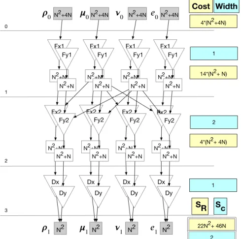
5.1 Protoimplementation of the step function from the Euler solver. . . 90 5.2 Polyhedral+dataflow graph for the Euler step function. . . 94 5.3 Iterator trees for the (a) original consToPrim1 and laplacian
computations, (b) laplacian after interchange and shift applied, and (c) final fused tree. . . 97 5.4 Performance results for the Euler step function on a Cori Haswell CPU
node. . . 102 5.5 Comparison of code variants for each box size with thread sweep from
1 to 64. . . 103 5.6 Performance results for the Euler step function on a NVIDIA Pascal
GPU. . . 104
6.1 Optimized code for the composed inspectors to convert COO matrices into the CSR, DSR, ELL, and CSB formats. . . 111 6.2 Optimized code for the conjugate gradient algorithm with SpMV
ex-ecutor of the CSR format. . . 112 6.3 Optimized code for the CPD algorithm with HiCOO variant of the
MTTKRP executor. . . 122 6.4 Performance results for the Conjugate Gradient algorithm on an Intel
Xeon CPU. . . 123 xvi
Pascal GPU. . . 123 6.6 Performance results for the CP-ALS algorithm on an Intel Xeon CPU. 124
NSCI – National Strategic Computing Initiatitive
ECP– Exascale Computing Project
DOE – Department Of Energy
NNSA – National Nuclear Security Administration
FLOP – Floating Point Operation
AMR – Adaptive Mesh Refinement
SAMR– Structured Adaptive Mesh Refinement
AST – Abstract Syntax Tree
IR– Intermediate Representation
COO – Coordinate Format
CSR – Compressed Sparse Row
CSC – Compressed Sparse Column
CSF – Compressed Sparse Fiber
ELL – ELLPack Format
BSR– Block-compressed Sparse Row
CSB – Compressed Sparse Block
HiCOO – Hierarchical Coordinate Format
PDFL – Polyhedral+Dataflow Language
PDFG – Polyhedral+Dataflow Graph
GeMM – Generalized Matrix Multiplication
LUD – Lower-Upper Decomposition
SVD – Singular Value Decomposition
MPP – Moore-Penrose Pseudoinverse
SOR – Successive Over Relaxation
ODE – Ordinary Differential Equation
PDE – Partial Differential Equation
SGD– Steepest Gradient Descent
SPD – Symmetric Positive Definite
CG – Conjugate Gradient
CPD – Canonical Polyadic Decomposition
PCA– Principal Component Analysis
GMG – Geometric Multigrid
AMG – Algebraic Multigrid
ILP – Integer Linear Programming
GCC – Gnu Compiler Collection
ICC – Intel Compiler Collection
TBB – Thread Building Blocks
DAG – Directed Acyclic Graph
CFG– Control Flow Graph
DFG – Dataflow Graph
DSA – Dynamic Single Assignment
SSA – Static Single Assignment
DSL – Domain Specific Language
eDSL – Embedded Domain Specific Language
PDFG – Polyhedral+Dataflow Graph
PDFL – Polyhedral+Dataflow Language
PEP – Polyhedral Expression Propagation
SCoP – Static Control Part
CFD – Computational Fluid Dynamics
FFT – Fast Fourier Transforms
α Step length in conjugate gradient computation
β Solution improvement in conjugate gradient computation
γ Conserved to primitive factor in Euler equations ∆ Laplace scalar operator
λ Normalization vector in Kruskal tensor ∇ Del operator for gradients
ρ Density in fluid dynamics applications R Set of all real numbers
Z Set of all integers Σ Summation operator
Q
Product operator
⊗ Kronecker product operator Hadamard product operator † Moore-Penrose pseudoinverse
X General tensor
CHAPTER 1
INTRODUCTION
The solutions to many important scientific, engineering, and national security challenges require improvements in the software stack to achieve the computational ef-ficiency necessary for large scale modeling and simulation applications. The National Strategic Computing Initiative (NSCI) prioritizes fields such as molecular dynamics, material science, advanced manufacturing, and precision medicine [1]. The Exascale Computing Project (ECP) is an associated effort to build computational tools that support advances in these fields. Computational efficiency is determined by the number of resources required by an application. More efficient computation means that more data can be processed in less time or with fewer resources. This work aims to improve computational efficiency in scientific applications.
Compilers are crucial components of the software stack, and are responsible for translating code implemented in high-level programming languages to architecture-specific assembly code. During this translation, the computational efficiency of the application can be improved by performing the appropriate set of code optimizations and transformations. The best sequence of optimizations depends on the target architecture. There has been an increase in architecture variability and complexity in recent years. CPU memory hierarchies have become more complex, and scientific applications often target alternative architectures including graphics processors and
field-programmable gate arrays. More compiler internal representations are required to select and apply effective code transformations.
Dataflow optimizations are especially beneficial for memory bound applications, which are those that move relatively large quantities of data per each unit of arith-metic computation. This low computational intensity means that processors spend significant amounts of time waiting for data to become available for computation. By contrast, compute bound applications are limited by the rate at which processors can perform arithmetic operations on data that are already available [2].
Significant performance gains in memory bound applications can be achieved by dataflow optimizations that reorganize computations and reduce storage require-ments. Scientific applications contain common computational patterns that enable these types of optimizations, such as linear algebra operations, or stencil computa-tions. The calculations are typically implemented as a series of nested loops over the data, with each loop nest computing a portion of the solution. To take advantage of these patterns, computations performed across large data domains are often dis-tributed across many compute nodes in a network or cluster. The performance of shared memory programs is crucial for scalability since the time and energy lost to poor single node performance is multiplied when the code is distributed.
Memory access patterns are critical to application performance and scalability. Applications with predictable data accesses and control flow patterns can be statically analyzed and optimized at compile time. These applications have regular patterns and so are considered regular. Other applications that rely on pointers or other indirect memory access patterns cannot always be statically analyzed. Such applications are referred to as irregular. These computations may require run time information or domain specific knowledge to be successfully optimized [3]. Both classifications of
memory access patterns are considered in this work.
Transforming readable and maintainable application source code into fast and energy-efficient machine code is challenging for compilers, due in part to existing programming language designs. A unified representation grants programmers control over memory interactions and execution schedules, but burdens them with the respon-sibility to write efficient code. This is particularly difficult for domain experts with no background in computer science or software engineering. These users may instead wish to convert mathematical expressions into algorithmic representations without being concerned with programming abstractions or hardware performance. This separation of concerns enables domain experts to write algorithms and performance engineers to apply optimizations, resulting in performance portability. Achieving this portability requires trade-offs between memory storage and computation, which is important for computationally intensive science and engineering applications.
The effectiveness of dataflow optimizations greatly depends on the abstraction level at which the code is analyzed. Higher abstraction levels such as the source code better capture the intention of the computation. However, the source code representa-tion of scientific computarepresenta-tions should not be altered to enable optimizarepresenta-tions, improve performance, or target different hardware architectures. Such changes can make the source code difficult to understand, maintain, and update by domain scientists or engineers. Performing compiler optimizations at the instruction level can lead to ineffective dataflow optimizations. This leaves the programmer to perform dataflow optimizations at the source code level. Instead, transformations should be applied to a higher level intermediate representation (IR) within the compiler, or via an abstraction layer that enables a performance expert to tune the applications. These goals can be achieved by decoupling the algorithmic specification from the execution
schedule and data layout [4–6].
This research targets compiler transformations focused on dataflow optimizations for memory bound applications. A compiler intermediate representation was de-signed and developed to enable code transformations in existing applications using a combination of program analysis, performance modeling, and programmer feedback. Domain experts can implement computations in the provided specification language, while performance engineers can transform code by manipulating the intermediate representation. The dataflow optimizations were applied to improve the performance of finite difference and structured grid solvers, and sparse linear algebra applications. The specific research contributions are described in the following section.
1.1
Contributions
1. Development of the polyhedral+dataflow graph intermediate representation (PDFG-IR) that expresses execution schedules, dataflow, memory interactions, and program statements in a manner that expands the set of automated transforma-tions available to optimizing compilers. The polyhedral model is combined with macro-dataflow graphs to explicitly represent data requirements, including data type, domain, and size. The graphs encapsulate code with execution schedules and data mappings for both persistent and temporary storage spaces.
2. Definition and implementation of compiler transformations to modify the ex-ecution schedules and storage mappings of the specified computation. These operations include statement rescheduling, producer-consumer and read-reduce loop fusion, and other loop transformations, such as unrolling, splitting, and tiling. Storage reductions are determined using reuse distance and reachability
analyses. A memory allocation algorithm based on liveness analysis [7] is described that allocates sufficient space for those data that are live at each point in the computation.
3. Extension of the IR to support irregular applications using the inspector/ex-ecutor approach [8]. The inspector-exinspector/ex-ecutor method is applied when code or data transformations require run time support, including run time dependence analysis or data transformations. Both inspectors and executor components can be represented and optimized, by transforming both data and iteration spaces. Non-affine, data dependent loop bounds are represented byuninterpreted func-tions [9] and converted into explicit represetations at run time.
4. Development of an embedded domain specific language to construct the IR. Numerical algorithms are expressed in C++ using a combination of iterators, functions, constraints, spaces, and executable statements. An iteration space is composed of an iterator set and their corresponding boundary constraints. Data spaces are derived from access functions in the statements. A computation consists of an iteration space, execution schedule, and statement list. The PDFG-IR is generated from the eDSL specifications.
5. Generation of an internal performance model for each graph variant. Many different graph variants can be generated from an initial graph specification by applying the supported transformations. A performance model is generated for each variant that include estimates of floating point operations (FLOPs), memory throughput, and arithmetic intensity. The model can be used to reason about the performance of a given variant on a target architecture.
1.2
Dissertation Structure
The remainder of this dissertation is organized as follows. Chapter 2 provides background on the numerical methods targeted in this work, the polyhedral model and associated compiler technologies, sparse matrix and tensor representations, the inspector-executor approach, dataflow languages, and memory optimizations. The polyhedral+dataflow IR and its application to regular applications is described in Chapter 3. The polyhedral+dataflow language (PDFL) and PDFG-IR extensions to support irregular applications are detailed in Chapter 4.
The integration of PDFG-IR with a structured grid adaptive mesh refinement solver (SAMR) eDSL calledProtois described in Chapter 5. Case studies including conjugate gradient (CG) and canonical polyadic tensor decomposition (CPD) imple-mentations are performed in Chapter 6. A survey of related work is provided in Chapter 7. Finally, topics for future work are discussed, and conclusions are drawn in Chapter 8.
CHAPTER 2
BACKGROUND
This chapter provides an overview of the concepts applied in this work. The research has built on recent developments in polyhedral compiler frameworks [10–12], loop chains [13–15], domain specific languages [4–6], dataflow programming lan-guages [16–18], memory access optimizations [19–21], stencil-based partial differential equation (PDE) solvers [22–25], inspector/executor applications [26–28], code gener-ation with non-affine or data-dependent loop bounds [8, 29, 30], and sparse matrix or tensor optimizations [31–33]. The applications targeted for optimization by this work include numerical methods for mathematical solvers, scientific and engineering simulations, or data analytics.
2.1
Compiler Optimizations
A typical optimizing compiler consists of at least three stages. The source code in the chosen programming language is parsed and converted into an initial intermediate representation (IR), such as an abstract syntax tree (AST). The IR may undergo many transformations, and several different representations as the code progresses through a series of optimization passes. The final IR is passed to the code generator that then emits machine instructions for the target architecture. An example is the register transfer language (RTL) of the Gnu Compiler Collection (GCC). Finally, the
compiled code is linked with any external libraries to produce an executable binary file. An overview of this process is given in Figure 2.1.
The correctness of every transformation performed by a compiler must be guar-anteed. The soundness of an optimization assures that the runtime behavior of the program is not modified. This requirement forces conservative decisions to be made during static analysis passes that occur at compile time. These passes are applied by traversing the various internal representations in the middle-end of the compiler infrastructure. A trade-off between precision and compile time overhead exists for each optimization.
Compiler optimizations can be limited by the high level language semantics. The use of pointers in C, for example, presents a significant challenge to data dependence analyses. If the compiler cannot guarantee that two pointers do not address overlap-ping memory spaces within a reasonable amount of time, it must assume that the pointers are aliased. This assumption limits possible transformations, and therefore the run time performance.
Programmers may conservatively allocate more space than necessary, rather than formally analyzing the space requirements of an algorithm. A compiler that supports
Figure2.1:Processflowofanoptimizingcompilerwithparser(front),optimization passes (middle), code generator,and linker (back-endcomponents).
data transformations can help overcome such challenges by automatically reducing the amount of temporary storage allocated, or reordering the data into a form that is more efficient for the given computation and target architecture. The IR described in this work is designed to apply such transformations.
Unnecessary data movement at the application level consumes large quantities of time and energy. Memory interactions at this level are difficult to understand, reason about, and therefore optimize. Irregular applications are characterized by non-sequential memory access patterns or sparse data structures that cannot be statically analyzed in a straightforward manner. The problem is compounded by the difficulty of communicating dataflow information to the middle-end of an optimizing compiler. The methods to provide information such as data access mappings or read/write patterns are limited in existing programming languages.
Compiler IRs are data structures that represent a series of machine instructions coded in a programming language [34]. ASTs are recursive data structures that represent the syntactic structure and content of a program. A basic block is a sequence of instructions with no control flow (branches) except the entry and exit points. A control flow graph (CFG) describes execution order, and can be obtained by traversing the AST. Each CFG node represents a basic block of the program, and each edge indicates the transfer of control from one block to another. The CFG is translated into a static single assignment (SSA) form [35], such as GIMPLE in GCC or LLVM-IR in Clang.
Dataflow analysis is performed on the CFG to produce a dataflow graph (DFG). The flow of data blocks during program execution are described by the DFG structure. The SSA form enables more efficient data dependence analysis. Dataflow analysis is limited even in SSA form, and much of the data movement is left to the programmer
to define.
Programming languages such as C and Fortran do not provide the necessary dataflow information to the compiler middle-end. Two potential soultions to this problem are code annotations and embedded DSLs. The programmer can annotate the source code with pragmas or decorators, for example, to indicate vectorization opportunities, identify static control parts of programs (SCoPs), or provide dataflow information [36,37]. These annotations are ignored by the general purpose compilers. Irregular applications that require sparse or unstructured computations are im-portant in scientific simulations and analytics. These applications reduce data storage by only storing nonzero data elements [38]. The element locations are stored in index data structures, requiring indirect memory accesses. The resulting code contains data dependent loop bounds that cannot be statically analyzed by an optimizing compiler. The inspector/executor approach addresses this problem by enabling compiler transformations at run time. An inspector can observe data access patterns, perform dependece analysis, or apply run time data transformations. The executor performs the computationally intensive computation on the data transformed by the inspec-tor [27]. Statically optimized inspecinspec-tors and efficient execuinspec-tors can be produced at compile time [39].
2.2
Polyhedral Model
The polyhedral compilation model [40] is a mathematical framework for describing complex applications with multiple operations and loop nests in a compact form. An affine transformation is a linear mapping that preserves points, lines, and planes [41]. Loop iterations are represented as lattice points within a polyhedron. Affine
transfor-mations can be applied to the polyhedra, enabling loop optimizations such as fusion and tiling. The model provides a means of applying loop transformations based on affine spaces defined by integer sets. An iteration space that describes a loop nest can be considered an affine space, an integer set of tuples (i1,...,in) ∈Zn.
A loop nest can be represented with the following components:
1. Iteration Space: the set of statements in the section, and the loop iterations where instances of the statement are executed. These are specified with named union sets. An integer set, I, is defined as
I ={[i1, . . . , in]|c1 ∧ . . . ∧cm } (2.1)
Where i1, . . . , in are indices, or iterators, in the n dimensions of the set, and
c1, . . . , cm are the affine inequalities, or constraints, that bound the integers in the set. Integer sets are typically expressed as Presburger formulae [42].
2. Access Relations: The set of reads, writes, and may-writes that relate statement instances in the iteration space to data locations. These are represented by mapping functions or relations. An integer relation is denoted by the mapping
R={[i1, . . . , in] → [j1, . . . , jk]|c1 ∧ . . . ∧cm } (2.2)
Where (j1, . . . , jk) is the integer tuple in the destination set. A mapping from a dense matrix, A, accessed at indices (i, j), to a sparse matrix A’, for example, is defined as
RA→A0 ={[i, j] → [i0, j0]|0≤m < M ∧ (2.3)
i0 =row(m)∧ j0 =col(m)} (2.4)
Where M is the number of nonzero values, and row, col are the respective row and column indices.
3. Dependences: The set of data dependences that impose restrictions on the execution order, e.g., producer- consumer relationships. Dependences can be modeled with maps or edges in a dataflow graph. An array A, read at each point (t, i,j) of an iteration space I, would be represented by the mapping
RI→A={I[t, i, j]→A[i, j]} (2.5)
4. Schedule: The execution order of each statement instance can be represented by a lexicographically ordered set of tuples in a multidimensional space [43]. Lexicographic ordering (≺) is defined as
(a1, . . . an)≺(b1, . . . bm) ⇐⇒ ∃i|1≤i≤min(n, m) s.t. (2.6) (a1, . . . ai−1) = (b1, . . . , bi−1) andai < bi
A statement, S executed at every point in iteration space, I, would have the scheduling function
TI→S ={I[t, i, j]→[t,0, i,0, j]} (2.7)
instances and the corresponding execution order. Polyhedral optimizations change the execution schedule without affecting the set of statements that are executed [44]. Transformations that involve statement reordering include fission, fusion, skewing, interchange, reversal, and tiling. Polyhedral representations can be extracted from source code by analyzing loop bounds and array subscript expressions [45].
Polyhedral code generators such as CLooG [46,47] or Omega [48] apply algorithms that can construct an AST from polyhedra by combining if nodes for conditional statements,for nodes for loop nests, block nodes representing compound statements or basic blocks for loop bodies [43]. Transformations that can be applied outside of the polyhedral framework include loop unrolling, skewing, and tiling. Polyhedra are converted back into ASTs using quantifier elimination techniques for linear inequali-ties such as Fourier-Motzkin or Chernikova’s algorithm [49].
Compiler frameworks such as CHiLL [50] or PLuTo [10] have been built using the polyhedral model. The loop chain abstraction [13, 51] applies transformations to series of loops referred to as loop chains, and demonstrates the potential impact of these transformations on both regular and irregular applications. The loop chain compiler was built on the integer set library (ISL) [52]. The Polly [53, 54] interface for LLVM [55] has demonstrated the applicability of the polyhedral model within compiler optimization passes.
Domain specific languages (DSLs) target a particular problem space. Halide [4,56] and PolyMage [5, 57], for example, are DSLs built specifically for image processing pipelines. Constructing an entirely new compiler is a considerable software engineer-ing challenge, so DSLs are often embedded within existengineer-ing languages such as C++ or Python (eDSLs).
2.3
Dataflow Languages
The dataflow programming paradigm was motivated by the need to expose par-allelism [58]. Early dataflow architectures exhibited poor performance in cases of fine-grained parallelism. A study by Sterling et al. [59] indicated that balancing task granularity was the critical factor in the performance of dataflow programs. A hybrid dataflow / von Neumann approach has since emerged, allowing developers to benefit from both coarse-grained dataflow parallelism at the macro-level and fine-grained instruction level parallelism. Dataflow programming is similar to functional program-ming in that the code is free of side effects and variables can only be assigned once. In this research, the execution schedule as described in subsection 2.2, is determined by the data dependences from the dataflow graph.
A dataflow graph is an intermediate representation that follows the flow of data through a function or procedure to identify dependences. Statement level dataflow graphs are directed acyclic graphs with nodes at the iteration granularity. Macro dataflow graphs were introduced to coarsen the granularity by grouping iterations into a single node [60]. Functional representations of an application can be translated into macro dataflow graphs. This representation can be traversed to exploit parallelism and assist the associated code generation [61].
Prasanna et al. [62] take a hierarchical approach. Each macro node is scheduled for parallel execution on a machine, unlike the previous work that assumed sequential execution. The entire graph is then partitioned and scheduled for distributed memory execution.
2.4
Memory Optimizations
The clock speeds of microprocessors have increased exponentially since the advent of Moore’s law [63], however, off-chip memory performance has not achieved the same rate of improvement. Deeper memory hierarchies have been introduced to bridge the gap. The memory levels between the CPU registers and main memory, collectively referred to as cache, are larger but slower near the bottom, and faster but smaller toward the top. Cache replacement protocols are responsible for transferring blocks of data between cache and DRAM in an effort to ensure that the most frequently accessed data can be retrieved quickly. This leads to the concept of data locality [64]. Compilers are responsible for generating code that reduces both the number of cache misses and the impact of unavoidable misses. This can be accomplished by maximizing data reuse, and ensuring that data are stored contiguously for each process. Techniques to achieve these goals include automatic data layout [65–67], affine partitioning, and loop blocking or tiling. Lattice-based memory optimiza-tion [19, 68, 69] is an approach to affine partioptimiza-tioning. Polyhedral data reuse [20] and associative reordering [70] are other methods to improve data reuse. Contiguous data transformation techniques include permutation, strip-mining, and compiler-directed page coloring [71, 72].
2.5
Target Computational Patterns
This work targets a subset of scientific computing methods that share common computational patterns. Colella identified theseven motifs [73] of scientific computing as structured and unstructured grids, dense and sparse linear algebra, fast Fourier
transforms (FFT), particle interactions, and Monte Carlo simulations. This work fo-cuses on stencil computations within structured grids, and linear algebra applications.
2.5.1 Iterative Methods
Many mathematical problems cannot be solved analytically. Numerical methods are algorithms designed to solve systems of equations with arbitrary precision using successive approximations [74]. Iterative methods consist of an acceptable error threshold for convergence, and a maximum number of steps or iterations. An initial estimate can be provided, based on domain knowledge or assigned randomly. Open methods find the roots, or zeros, of a function within a fixed interval given an initial estimate. Open methods include bisection, Newton-Raphson, the secant, or Brent’s method [75], also known as the zeroin algorithm [76]. Open methods can be applied to linear or nonlinear systems. An example implementation of the Newton-Raphson method in C is given in Figure 2.2.
1 #define T 500 2
3 double tol = 1e-5; 4 double err = 1.0;
5 double x = x0; // Initial guess 6
7 for (t = 1; t <= T && fabs(err) >= tol; t++) {
8 // x(i+1) = x(i) - f(x) / f’(x)
9 err = func(x) / deriv(x);
10 x -= err;
11 }
2.5.2 Gradient Methods
Gradient methods compute derivatives to find local optima [77]. The gradient descent algorithm can be used to find minima, or the steepest ascent (hill-climbing) for maxima. Powell’s conjugate direction method [78] is an algorithm for finding local minima that is applicable when the function is discontinuous, non-differentiable, or no information about the derivative is available. It is an efficient, quadratic method (O(n2) convergence) that is often paired with Brent’s method as its search technique due to its linear time complexity.
The conjugate-gradient method is composed of three fundamental operations, scalar multiplication, sparse-matrix vector multiplication, and the inner product. The inner product of two vectors, denoted xTy, is computed as the scalar sum PN
i=1xiyi. The matrix, A, is symmetric positive definite (SPD), if xTAx > 0 for every nonzero vector,x. The domain of possible solutions to the unknown vector,x, can be expressed in the quadratic form, 12xTAx−bTx+c, where c is a scalar constant. The gradient, or first derivative, is f0(x) = 12ATx+1
2Ax−b. Since A is symmetric, this reduces to
f0(x) =Ax−b. Therefore, the system is solved by finding the vector, x, that sets the gradient to zero. In other words, f(x) is minimized when the gradient f0(x) = 0, or
Ax=b.
Gradient methods find this critical point by selecting an arbitrary initial solution,
x0, and making a series of steps, x1, x2, ..., xn, computing the residual after each, and stopping at some maximum number of iterations or until the error is within some acceptable tolerance with respect to the actual x. Each new search direction is constructed from the residual at each step of the CG algorithm. Successive directions are orthonormal to all previous search directions, ensuring that the same direction
will not be followed more than once, and thus accelerating convergence.
Conjugate gradient is among the most popular methods for solving large systems of linear equations in the form, Ax =b, where x is an unknown vector to be solved, b is known, and A is a square (N ×N), SPD matrix of known values. [79]. Iterative methods like CG or Jacobi are best-suited to systems involving sparse matrices. Dense matrices can be solved more efficiently using direct methods such as factorization and backsubstitution, e.g., lower-upper (LU) decomposition [80]. Multifrontal methods are an efficient approach to LU factorization in sparse systems [81].
The CG algorithm is summarized in equations 2.8–7, where the zero subscript represents the initialization step, i is the current iteration, and n the maximum number of iterations. The vectors, d, r, s, x represent the search direction, residual, step, and approximate solution, respectively. The scalarαis the step length, andβthe improvement in the solution over the previous iteration. The process continues until the residual error falls below a given threshold, orn iterations have been performed.
d0 =r0 =b−Ax0 (2.8) si =Adi−1 (2.9) αi = rT i−1ri−1 dT i−1si (2.10) xi =xi−1+αdi−1 (2.11) ri =ri−1−αsi (2.12) βi = riTri rT i−1ri−1 (2.13) di =ri+βdi−1 (2.14)
remainder of the algorithm consists of one matrix-vector product (equation 6.2), five dot products, three vector additions, and three scalar-vector products per iteration.
2.5.3 Finite Difference and Volume Methods
Conservation problems in physics are often expressed as partial differential equa-tions, that must be solved with computational methods when analytical solutions are unavailable. The Navier-Stokes equations describe the flow of viscous fluids, including the conservation of mass, energy, and momentum [82]. The general form is given as
∂U
∂t +∇ ·
~
F(U) = 0 (2.15)
whereUis the vector of conserved unknowns,t is time,∇is the differential operator nabla, and F~ is the flux dyad tensor in each spatial direction.
These equations can be solved numerically by approximating a sequence of alge-braic equations at discrete locations on a structured grid over the spatial domain. The point-wise approximations are known as finite-differences, and are derived from Taylor-series expansion, df dx i = f(xi+1)−f(xi−1) 2∆x +O(∆x 2) (2.16)
where i is a discrete grid location in one dimension, and O(∆x2) is the truncation error introduced by a continuous equation approximation in a discretized algebraic form. The error magnitude is a quadratic function of the grid spacing, ∆x.
The finite-volume method is an alternative tofinite-difference, where the solution is approximated by integrating over a small control volume, Vi defined by the grid.
Integrals are defined as ∂ ∂t Z Vi Udx+ Z Vi ∇ ·~Fdx= ∂ ∂t Z Vi Udx+ Z ∂Vi ~ F·nˆdS = 0 (2.17)
with the equation on the right obtained by applying Gauss’ divergence theorem. The ∇ ·~F integral is converted into the normal component integral of the ~F vector over the control volume surface, where ˆn is a unit normal vector pointing outward from the volume. The change of the unknown vector,Uover time is equal to the total flux of F~ crossing the surfaces in the same time span.
Equations are solved in the finite-volumeapproach by discretizing the volume and approximatingF~ on the control volume faces from the values stored in adjacent cells. The finite-volume method incurs a truncation error and implied stencil width. The advantage is that a local conservation property ensures discrete conservation across the entire domain as in the actual PDEs. Figure 2.3 depicts this process in two dimensions (x,y).
Figure2.3:Cellfluxesacrosssurfacefacesofcontrolvolume.
PDEs are solved inpractice by dividingthe grid intodiscrete cells, iteratingover them, and evaluating the algebraic equations for a specified number of iterations. Large domains can be partitioned into smaller pieces referred to as boxes. These
boxes are padded with layers of ghost cells to reduce communication overhead and enable parallel execution.
2.5.4 Structured Grid Methods
Iterative methods can provide an effective means for solving large systems of equations. However, convergence can be slow, requiringO(N2) iterations, which can be unacceptable for some problems. Multigrid methods allow iterations to change from a fine grid to a coarse grid, with the benefits of reducing convergence to O(N) iterations and improving performance. Multigrid is particularly effective on sparse, symmetric systems [83]. A structured grid solver for the Euler equations is described in Chapter 5.
The Jacobi, Gauss-Seidel, or successive over-relaxation (SOR) stencil computa-tions can be applied at each step to solve a linear system Ahx = bh to obtain xh, whereh corresponds to the current grid size [74]. These iterative methods are derived from the discretized Taylor series of the function, f, represented by the matrix, A.
Ath i,j = 1 4 Ath−1 i+1,j +A t−1 hi−1,j +A t−1 hi,j+1+A t−1 hi,j−1 −h 2A i,j (a) Athi,j = 1 4 Ath−1 i+1,j +A t hi−1,j +A t−1 hi,j+1+A t hi,j−1 −h 2 Ai,j (b) Ath i,j = w 4 Ath−1 i+1,j +A t hi−1,j +A t−1 hi,j+1 +A t hi,j−1 −h 2A i,j + (1−wAth−1 i,j) (c) (2.18)
Jacobi is an iterative method that updates the current matrix using only values from the previous time step as seen in Equation 2.18(a). Gauss-Seidel (b) takes advantage of the fact that the values for previous spatial iterations (i-1 and j-1) have already been computed and can perform in place updates, reducing the amount of storage that must be allocated and accelerating convergence. Successive
over-relaxation (c) is a Gauss-Seidel refinement that includes a weight term, 1 < w < 2 that moves the approximation further in the relaxation direction to reduce the number of iterations required for convergence. The h2Ai,j term in all three equations is the quadratic error.
The use of recently updated values from the same time step in Gauss-Seidel and SOR introduces a race condition resulting in code that is difficult to parallelize. This is resolved by applying red-black ordering. A grid point (i, j) is marked red if the sum (i +j) is even and black if it is odd. The red points are updated in the first pass and the black points by reading the red values. Implementations of these smoothing stencils in the C language are shown in Figure 2.4.
1 for (t = 1; t <= T; t++) { 2 for (i = 1; i <= N; i++) { 3 for (j = 1; j <= N; j++) { 4 A[t,i,j] = (A[t-1,i+1,j] + 5 A[t-1,i-1,j] + A[t-1,i,j +1] + 6 A[t-1,i,j-1]) * 0.25; 7 } } } (a) Jacobi 1 for (t = 1; t <= T; t++) { 2 for (i = 1; i <= N; i++) { 3 for (j = 1; j <= N; j++) { 4 A[t,i,j] = (A[t-1,i+1,j] + 5 A[t,i-1,j] + A[t-1,i,j+1] + 6 A[t,i,j-1]) * 0.25; 7 } } } (b) Gauss-Seidel 1 for (t = 1; t <= T; t++) { 2 for (i = 1; i <= N; i++) { 3 for (j = 1; j <= N; j++) { 4 A[t,i,j] = (A[t-1,i+1,j] + 5 A[t,i-1,j] + A[t-1,i,j+1] + 6 A[t,i,j-1]) * w * 0.25; 7 A[t,i,j] += (1 - w * A[t-1][i][j]); 8 } } }
(c) Successiveover relaxation
2.5.5 Tensor Decomposition
Higher dimensional problems that cannot be represented by matrices are stored in tensors. The rank R, of a tensor X, is the minimum number of indices required to uniquely identify every element in the tensor. The order, d is the number of modes, or dimensions in the tensor. Tensors are a generalization of matrices to higher orders, where scalars are zero order, vectors are first order, and matrices are second order. Tensors can be simplified by decomposing them into a sequence of operations on lower order structures. Tensor decomposition is a generalization of matrix decomposition techniques such as singular value decomposition (SVD) or principal component analysis (PCA) [84].
A tensor can be matricized, for example by taking a slice, X(:,j,k). In general, a tensor X ∈ Rn1×...×nd can be matricized into a matrix A ∈
RN1×N2|N1N2 =
n1. . . nd. A tensor can be decomposed into the sum of rank one tensors (vectors),X≈
PR
r=1x1r◦. . .◦xdr. The corresponding factor matrices,X(1) = [x11. . .x1r], . . . ,X(d)= [xd1. . .xdr] are formed from the component vectors, where X(n) is the mode-n ma-tricization. Given a third order tensor, X ∈ RI×J×K, let A
I×R,BJ×R,CK×R denote the factor matrices and X(i,j,k) each tensor element.
The Kronecker product, A ⊗B is a generalization of the outer, or Hadamard product, resulting in a block matrix of size IJ ×R2. The Khatri-Rhao product is the column-wise Kronecker product, AB= [A(:,1)⊗B(:,1). . .A(:, R)⊗B(:, R)] producing a block matrix with dimensions IJ ×R. The CPD produces one factor matrix per mode.
X(1) ≈A(CB)| →A≈X(1)(CB) (2.19)
X(2) ≈B(CA)| →B≈X(2)(CA) (2.20)
X(3) ≈C(BA)| →C≈X(3)(BA) (2.21)
This computation requires three applications of the matricized tensor times Khatri-Rhao product (MTTKRP), the bottleneck in many tensor decomposition applications. The columns of the factor matrices are often normalized to a length of one, with weights stored in a vector λ ∈ RR, where the matrix Λ = diag(λ). Factor matrices are held constant while a new one is computed for the current mode. This reduces the problem to linear least-squares, leading to the alternating least squares (ALS) algorithm for computing CPD. The minimization problem can be expressed in the form min
˜ A
kX(1)−A˜(CB)>kF where ˜A=A·Λ and k · kF is the Frobenius norm. The optimal solution is given by
˜
A=X(1)[(CB)|]† =X(1)(CB)(C|C∗B|B)† (2.22)
where † denotes the Moore-Penrose pseudoinverse. The pseudoinverse reduces the complexity since only an R×R matrix is needed, rather than J K×R.
The pseudoinverse is computed by applying the SVD to decompose the matrix A into two unitary matrices U, V, and a diagonal matrix Σ, such that A = UΣV∗, where * represents the conjugate transpose, or simply the transpose for real valued matrices. The values in Σ are singular, and the columns of U, V are the left and right singular vectors, respectively. These are approximations of the eigenvalues and eigenvectors. The Moore-Penrose pseudoinverse is defined asA†=VΣ†U∗ [85].
matrices can be initialized to zero, randomly, or to theR leading left singular vectors of X(n). The large quantities of data produced by the Khatri-Rhao products are known as the intermediate data explosion problem [86]. The source code for a possible implementation of the CPD algorithm focused on the MTTKRP kernel is given in Figure 2.5. The code is for a four dimensional tensor,X, of shape (I,J,K,L) and rank, R, with factor matrices A, B, C, D. The tensor and factor matrices are all dense in this example.
The generalized CP-ALS decomposition algorithm into rank, R, components, for anNth order tensor,X, of shape (I1,I2,. . . ,IN), with maximum number of iterations, T, is given in Figure 2.6. The algorithm produces the normalization vector, λ, and factor matrices,A1,A2,. . . , AN. 1 for (i = 0; i < I; i++) 2 for (j = 0; j < J; j++) 3 for (k = 0; k < K; k++) 4 for (l = 0; l < L; l++) 5 for (r = 0; r < R; r++) 6 A[i,r] += X[i,j,k,l]*B[j,r]*C[k,r]*D[l,r];
Figure2.5: SourcecodeforMatricizedTensorTimesKhatri-Rhaoproductforfourth ordertensor.
2.6
Sparse
Matrix
Formats
The particular structure of a matrix can be exploited to apply more efficient solving techniques to improve computational performance. Diagonal, or banded matrices are sparse, except for bands around the main diagonal. The distance from the main diagonal of the most distant value isknown asthe bandwidth. Tridiagonal
1 function cp_als(X, R) { 2 for (n= 1, . . . , N) { 3 An=rand(In×R) 4 } 5 for (t= 1, . . . , T∧ > τ) { 6 for (n= 1, . . . , N) { 7 V ←A>1A1∗. . .∗A>n−1An−1∗A>n+1An+1∗. . .∗A>NAN 8 An ←X(n)(A1. . .An−1An+1. . .AN)V† 9 λ← kAnkF 10 An ←An/λ 11 } 12 =fit(t)−fit(t−1) 13 } 14 return λ, A1, A2, . . . , AN 15 }
Figure 2.6: CP-ALS decomposition algorithm with R components for Nth order tensor, X.
matrices,forexample,haveabandwidthof3andoccurfrequentlyinengineering applications. The Thomas algorithm [87] can efficiently solve tridiagonalmatricxes.
Symmetricmatricesrequireonlyhalfoftheelementstobestored,sinceeachvalue
aij =aji,andcanbeefficientlysolvedusingCholeskydecompositionwithelimination trees [88]. The Cholesky algorithm has the additional constraint that the matrix be positive definite, meaning the scalar value x∗Ax is strictly positive for all positive columnvectors, x.
Storingonlythenonzerovaluesof amatrixcansavesigificantmemoryspace. Let N denote the number of rows and columns in the matrix, A, and M the number of nonzerovalues. The simplestwaytorepresentasparsematrix istostorethe nonzero values, and the coordinates (i,j) of each nonzero. This is known as the coordinate (COO) format [89]. This format is common in many popular repositories, such as the Matrix Market format inthe SuiteSparse matrix collection [90] or the FROSTT sparse tensor repository[91].
The COO format reduces the storage requirements from O(N2) to 3 × O(M) =
O(M). The COO format stores the same rows and columns multiple times, resulting in wasted space. The row array can be compressed into a row pointer (rp), or the columns can be compressed into a column pointer. The corresponding formats are known as compressed sparse row (CSR) and compressed sparse column (CSC), respectively [92].
The CSR and CSC formats can be compressed further if the matrix contains many rows or columns that contain only zeros. Only the indices of the rows or columns that contain nonzeros need to be stored for such matrices. In the case of CSR, the row pointer (rp) is compressed and a new array of compressed row indices is stored. This format is referred to as doubly-compressed sparse row (DSR) [93]. The choice of where to compress rows or or columns depends on which will yield a better compression.
Blocked sparse matrices can be efficiently represented by the blocked compressed formats. A matrix is block sparse when the nonzero values are clustered together in adjacent rows and columns. The matrix is divided into small dense blocks containing at least one nonzero element, and padded with zeros. The arrayA prime consists of all such nonzero blocks. Thebcol array stores the column of the upper left element of each nonzero block, and thebrow auxiliary vector has one element per block row, indicating the first element index of the row in the original matrix A.
The compressed sparse block format (CSB) [94] shares the data locality benefits of the BSR and BSC formats, but without the need to store dense sub-blocks that are padded with zeros. The nonzero values are instead rearranged so that they can be traversed in a block order, such as the Z-morton sorting used in octrees [95]. The format requires five auxillary arrays, one for the block pointers (analogous to the row pointer in CSR), and two each for the block row and column indices, and the element
row and column indices within each block.
The diagonal sparse matrix format (DIA) [96] is suitable for matrices with nonzero values near the main diagonal, such as the banded matrices in the previously described tridiagonal computations. The offsets from the main diagonal are stored in an auxiliary array. The ELLPACK format (ELL) [97] uses a 2-dimensional matrix with the maximum number of nonzero elements per row, and rows with fewer nonzero elements are padded with zeros. An auxiliary column matrix stores the column indices for the nonzeros. When most rows have a similar number of nonzero values, the ELL format is more efficient because of a fixed number of iterations and lack of indirect memory accesses. An example illustrating several of these matrix formats is given in Figure 2.7.
Tensor storage can be optimized by considering the data sparsity structure. The coordinate (COO) format can be generalized to sparse tensors by storing the coordi-nates for each mode. The compressed sparse fiber (CSF) format is a generalization of the CSR and CSC formats for matrices [98]. The HiCOO format is a generalization of the CSB format applied to tensors [33]. CSF is a mode-specific format, meaning that the resulting data structure is different depending on the mode compression order. The COO and HiCOO formats are mode-generic, so the nonzero values can be accessed in any order. Sparse tensor formats are summarized in Figure 2.8.
CHAPTER 3
POLYHEDRAL+DATAFLOW GRAPH INTERMEDIATE
REPRESENTATION
This chapter presents an intermediate representation for loop chain schedules, and data mappings, a methodology for minimizing temporary storage requirements, and a cost model for comparing different schedules and mappings.
The approach provides a visual interface to aid the performance expert in guiding polyhedral code transformations paired with storage mapping optimizations. In this work we explore the concept of a polyhedral+dataflow graph (PDFG). Based on macro dataflow graphs, PDFGs express dataflow at a high-level using sets of statements, include information about the data being passed between nodes, and use layout to express the execution schedule. This approach is unique in that it includes fine-grained information about memory interactions, while the graph itself remains coarse-grained. Cost models have been used to compare the anticipated performance of macro dataflow graphs consistently since their inception. Given that the goal of many of these graphs is to identify parallelism opportunities, most of the cost models focus on execution cost of computation nodes [60], and the communication costs associated with the adjacent edges.
The novel contributions described in this chapter include (1) a procedure to generate PDFGs given annotated source code, (2) a set of scheduling and data
Figure3.1:Overviewofthethreecodegenerationphasesusingloopchainpragmasand thepolyhedral+dataflowgraphmethodandassociatedcostmodel.
transformations for PDFGs, (3) a systematic approach to minimizing temporary storage requirements within graph nodes after fusion, (4) an approach for reducing storage allocations in the entire PDFG using liveness analysis, (5) a high-level cost model useful for comparing different graphs and execution schedules, and (6) a comparison of two overlappedtiling approaches.
3.1
Polyhedral+Dataflow
Graphs
A PDFG is a visual representation of a computation highlighting data depen-dences. Itcanbeconsideredatypeofmacro-dataflowgraph[60]. Traditionaldataflow graphsrepresent data dependences atafine-grained level,typically perstatement or machine instruction. PDFGs differ from existing dataflow graphs in three primary ways:
1. all iterations of a given loop nest are grouped into a single macro node,
2. data is explicitly represented as a node or set of nodes, and
3. the execution schedule is expressed as part of the graph layout.
This section describes the individual components of a PDFG, the expression of the execution schedule using graph layout, and a cost model to compare the potential performance of different graph variants. PDFGs form an intermediate representation that expresses both the execution schedule and dataflow requirements of an application kernel.
This chapter presents the graph IR, methods to transform them by manipulating the underlying polyhedral model, techniques to perform storage reductions, and code generation to produce optimized code. Optimization plans can be visualized, displaying intermediate steps, and the impact of transformations are clearly visible.
3.1.1 Graph Components
A polyhedral dataflow graph (PDFG) represents both the execution schedule and the dataflow requirements of a computation. A PDFG is defined as G = (V, E), where V = (S, D, T) and E the directed edges. S is the set of statement nodes, D
the data nodes, and T the transformation nodes. The source and destination node types incident to an edge determine the operation being represented. For example, an edge from a data node to a statement node indicates reading data, and an edge from a transformation node to a statement node indicates that the iteration space will be transformed by applying the corresponding relation. The edges indicate the flow of data between statement nodes, and therefore the coarse-grained execution schedule.
Statement nodes, inverted triangles in the graph, represent ordered sets of state-ments. They encapsulate the iteration domain, statements within the block, location within the global schedule as an iteration vector or tuple, and the data mapping, referencing the data spaces that are read and written during statement execution. The iteration domain of a statement node is represented using the polyhedral model and the location within the global schedule is maintained using a scattering function. This function determines the fine-grained execution schedule. Each node, s in S, corresponds to a basic lock or loop nest in the code.
The data nodes, depicted as rectangles, abstract storage spaces and consist of the type, range of values, the domain of indices that access it, and the size. The latter can be inferred from the domain of the statement node that writes the data. The space described in the graph corresponds to local space requirements and not actual memory allocations. The memory allocation and associated mapping are created during code generation. Each node, d in D, represents a data space in the program that will be mapped to memory by a storage mapping function.
Op1 N2+N N2+4N (a) M * N N * M (b)
Figure 3.2: Summary of graph components, including edges, data, statement, and transformationnodes.
The graph components are summarized in Figure 3.2. The node labeled N2 +4N
represents a data space with that cardinality. There are two classes of data nodes, persistentand temporary. Persistent dataare accessedoutsideofthe function
represented by the graph, either as inputs or outputs, and therefore have a fixed storage mapping. Temporary values are allocated and accessed only within the scope of the graph or loop chain. Persistent data nodes are shaded gray, and temporary or local data retain a white background. The N2+N space is temporary.
The statement node, Op1 in Figure 3.2(a) represents a code block that performs some operation. The incoming edge indicates that the block reads the persistent data, computes the results, and writes them to temporary storage. The contents of statement nodes are retrieved from loop bodies.
Arbitrary transformation functions can be introduced with transformation nodes, denoted in the graph as dashed boxes. Iteration space transformations are speci-fied beginning with a T and data transformations with an R by convention. The transformations are expressed as relations using Presburger arithmetic. The node in Figure 3.2(b) transposes the persistent data space, N*M to one ofM*N. Note that if that transformation were placed between two statement nodes, the result would be a loop interchange of the corresponding iteration spaces.
This polyhedral+dataflow representation support sparse data structures as well. Sparse data structures are important in many applications, including scientific com-puting, graph analysis (e.g., data science or social media networks), and machine learning. The code for these applications often results in irregular memory access patterns caused by multiple levels of indirection, for example with index arrays such asA[col[i]]). These patterns can result in poor performance due to reduced data locality. Data-dependent loop bounds and indirect memory accesses rely on data that are unknown until run-time, making static analysis difficult.
Uninterpreted functions are realized as explicit functions that satisfy the associ-ated constraints at run time. The computational kernel that requires the explicit
function is known as an executor, and the kernel that generates the data is an inspector. Inspectors are often hand-written, but both executors and inspectors can be generated by optimizing compilers, including the polyhedral model. The performance of many applications, including inspectors, can be significantly improved by decreasing temporary storage and thereby reducing memory traffic.
3.1.2 MiniFluxDiv Benchmark
The MiniFluxDiv benchmark [99] is used as an application exemplar to demon-strate this approach. The benchmark was chosen because it captures some of the complexity of full-scale simulation-based applications. MiniFluxDiv has been an-notated using loop chain pragmas [14]. The loop chain annotations provide the information required to achieve a separation of concerns among statements, schedule, and storage mappings. MiniFluxDiv is modeled after finite difference applications such as those written with the Chombo framework [100]. The benchmark focuses on the shared-memory portion of a single time step in an iterative solve. The input is a 3D, immutable data structure padded with a layer of ghost cells (2 deep). The domain is broken into a set of independent subdomains called boxes. Boxes are decomposed into cells; 163 cells is a typical box size, but larger box sizes are desirable to reduce the space required for ghost cells. We explore box sizes of 163 cells and 1283 cells in this work. Each cell represents a vector of five components, including density (ρ), energy (e), and the velocity in each direction (u, v,w).
The original implementation is a series of parallel loops. There are three loops for each dimension of the problem. The first loop performs a partial flux. This calculation results in face values, meaning that when the partial flux is calculated in the x-direction, a value is required for each border between cells. The second loop
completes the flux calculation using data from the corresponding velocity components in each direction to produce partial fluxes. These steps are referred to as Fx1 and
Fx2. The fluxes in the y- and z- directions are referred to as Fy1,Fy,Fz1, andFz2, respectively. The third loop calculates the differences between flux values and saves a cell-centered value at each point.
Each of the operations is applied to all five components. A naive implemen-tation results in a series of 45 parallel loop nests. The performance baseline is hand-optimized to reduce the number of loops.
Loop Chains
A loop chain is a series of loop nests that perform operations on shared data [51]. The loop chain abstraction captures this pattern and promotes decoupling of the execution schedule from the algorithmic primary expression. The abstraction can be implemented in a variety of ways: domain specific languages, libraries, or code annotations. A loop chain pragma language has been developed and a restricted version of it is used in this chapter [14].
The first column in Figure 3.1 demonstrates how the pragmas are added. The out-ermost pragma, omplc parallel(fuse), indicates the start of a loop chain and the schedule that should be applied, i.e., fuse. Each loop nest within the chain is la-beled with a pragma, indicating its domain. The pragmadomain(0:X+1,0:Y,0:Z), for example, indicates that iterator x has domain 0 through X+1 (inclusive). Data read and write patterns are specified in the pragma following the with clause.
A loop chain compiler has been implemented by Bertolacci et. al [14] that uses the pragma specifications to apply a variety of transformations to the original application code, including shifts/skews, fusion, tiling, and wavefront. In the existing tool, the
data access patterns help the compiler to ensure the legality of transformations, but is not used to optimize data accesses or temporary storage.
3.1.3 Execution Schedule
The edges of the graph indicate a partial execution schedule based on data de-pendences. The graph layout expresses the execution schedule. Graphs are executed from left to right, and top to bottom. Statements within the nodes are executed over the domain in lexicographical order. An exception is made after fusion operations. In this case any shifting will be automatically applied to ensure legal execution.
The original MiniFluxDiv schedule over a 2D domain is represented by the PDFG provided in Figure 3.3. The graph is organized into four columns, one for each component in the 2D space. The persistent data nodes in the top row labeled ρ0,
u0, etc. represent the initial input data for each box. Similarly, the persistent data nodes along the bottom, e.g., ρ1, u1, etc., contain the resulting output data. The input nodes are of size N2 + 4N, and the output nodes N2, the difference is due to ghost cells.
The first face-centered flux loop is represented by the statement nodes labeled
Fx1. Note that the velocity component of the Fx1 statement node, u, is read by the Fx2 statement nodes for all components. The same is true for Fy1(v). This dependence pattern is common in CFD applications, and is necessary to obtain realistic performance results.
3.1.4 Cost Model
A cost model is derived using the data nodes in PDFGs. Two primary metrics are calculated: the total amount of data read (SR), and the maximum number of streams
Fx1 N2+N Fx1 N2+N Fx1 N2+N Fx2 Fx2 Fx2 Dx Dx Dx Dx
𝝆
0 N2+4Nu
0 N2+4N𝝂
0 N2+4N𝑒
0 N2+4N Fx1 N2+N𝝆
1 N2 N2𝝂
1 N2𝑒
1 N2 N2+N N2+N N2+N N2+N Fx2 Fy1