Mining Contrast Subspaces

(1)

Wright State University

CORE Scholar

Kno.e.sis Publications

The Ohio Center of Excellence in Knowledge-

_{Enabled Computing (Kno.e.sis)}

5-2014

Mining Contrast Subspaces

Lei Duan

Guanting Tang

Jian Pei

James Bailey

Guozhu Dong

Wright State University - Main Campus, [email protected]

See next page for additional authors

Follow this and additional works at: https://corescholar.libraries.wright.edu/knoesis

Part of the Bioinformatics Commons, Communication Technology and New Media Commons,

Databases and Information Systems Commons, OS and Networks Commons, and the Science and Technology Studies Commons

Repository Citation

Duan, L., Tang, G., Pei, J., Bailey, J., Dong, G., Campbell, A., & Tang, C. (2014). Mining Contrast Subspaces. Lecture Notes in Computer Science, 8443, 249-260.

https://corescholar.libraries.wright.edu/knoesis/380

This Conference Proceeding is brought to you for free and open access by the The Ohio Center of Excellence in Knowledge-Enabled Computing (Kno.e.sis) at CORE Scholar. It has been accepted for inclusion in Kno.e.sis Publications by an authorized administrator of CORE Scholar. For more information, please contact [email protected].

(2)

Authors

Lei Duan, Guanting Tang, Jian Pei, James Bailey, Guozhu Dong, Akiko Campbell, and Changjie Tang

(3)

Mining Contrast Subspaces

⋆

Lei Duan1,6, Guanting Tang2, Jian Pei2, James Bailey3, Guozhu Dong4, Akiko Campbell5_{, and Changjie Tang}1

1

School of Computer Science, Sichuan University, China

2 _{School of Computing Science, Simon Fraser University, Canada} 3

Dept. of Computing and Information Systems, University of Melbourne, Australia

4 _{Dept. of Computer Sci & Engr, Wright State University, USA} 5

Paciﬁc Blue Cross, Canada

6

State Key Laboratory of Software Engineering, Wuhan University, China {leiduan, cjtang}@scu.edu.cn, {gta9, jpei}@cs.sfu.ca,

[email protected], [email protected], [email protected]

Abstract. In this paper, we tackle a novel problem of mining contrast

subspaces. Given a set of multidimensional objects in two classesC+and

C₋and a query objecto, we want to find top-ksubspacesSthat maxi-mize the ratio of likelihood ofoinC+against that inC−. We demonstrate that this problem has important applications, and at the same time, is very challenging. It even does not allow polynomial time approximation. We present CSMiner, a mining method with various pruning techniques. CSMiner is substantially faster than the baseline method. Our experi-mental results on real data sets verify the effectiveness and efficiency of our method.

1 Introduction

Imagine you are a medical doctor facing a patient having symptoms of being overweight, short of breath, and some others. You want to check the patient on two speciﬁc possible diseases: coronary artery disease and adiposity. Please note that clogged arteries are among the top-5 most commonly misdiagnosed diseases. You have a set of reference samples of both diseases. Then, you may naturally ask “In what aspect is this patient most similar to cases of coronary artery disease and, at the same time, dissimilar to adiposity?”

The above motivation scenario cannot be addressed well using existing data mining methods, and thus suggests a novel data mining problem. In a multidi-mensional data set of two classes, given a query object and a target class, we

⋆

This work was supported in part by an NSERC Discovery grant, a BCIC NRAS Team Project, NSFC 61103042, SRFDP 20100181120029, and SKLSE2012-09-32. Work by Lei Duan and Guozhu Dong at Simon Fraser University was supported by an Ebco/Eppich visiting professorship. All opinions, ﬁndings, conclusions and recommendations in this paper are those of the authors and do not necessarily reﬂect the views of the funding agencies.

(4)

want to find the subspace where the query object is most likely to belong to the target class against the other class. We call such a subspace acontrast subspace since it contrasts the likelihood of the query object in the target class against the other class. Mining contrast subspaces is an interesting problem with many important applications. As another example, when an analyst in an insurance company is investigating a suspicious claim, she may want to compare the sus-picious case against the samples of frauds and normal claims. A useful question to ask is in what aspects the suspicious case is most similar to fraudulent cases and different from normal claims. In other words, finding the contrast subspace for the suspicious claim is informative for the analyst.

While there are many existing studies on outlier detection and contrast min-ing, they focus on collective patterns that are shared by many cases of the target class. The contrast subspace mining problem addressed here is different. It fo-cuses on one query object and finds the customized contrast subspace. This critical difference makes the problem formulation, the suitable applications, and the mining methods dramatically different. We will review the related work and explain the differences systematically in Section 2.

To tackle the problem of mining contrast subspaces, we need to address several technical issues. First, we need to have a simple yet informative contrast measure to quantify the similarity between the query object and the target class and the diﬀerence between the query object and the other class. In this paper, we use the ratio of the likelihood of the query object in the target class against that in the other class as the measure. This is essentially the Bayes factor on the query object, and comes with a well recognized explanation [1].

Second, the problem of mining contrast subspaces is computational chal-lenging. We show that the problem is MAX SNP-hard, and thus does not allow polynomial time approximation methods unless P=NP. Therefore, the only hope is to develop heuristics that may work well in practice.

Third, one could use a brute-force method to tackle the contrast mining problem, which enumerates every non-empty subspace and computes the con-trast measure. This method, however, is very costly on data sets with a non-trivial dimensionality. One major obstacle preventing effective pruning is that the contrast measure does not have any monotonicity with respect to the subspace-superspace relationship. To tackle the problem, we develop pruning techniques based on bounds of likelihood and contrast ratio. Our experimental results on real data sets clearly verify the effectiveness and efficiency of our method.

The rest of the paper is organized as follows. We review the related work in Section 2. In Section 3, we formalize the problem, and analyze it theoretically. We present a heuristic method in Section 4, and evaluate our method empirically using real data sets in Section 5. We conclude the paper in Section 6.

2 Related Work

Our study is related to the existing work on contrast mining, subspace outlier detection and typicality queries. We review the related work brieﬂy here.

(5)

Contrast mining discovers patterns and models that manifest drastic diﬀer-ences between datasets. Dong and Bailey [2] presented a comprehensive review. The most renowned contrast patterns include emerging patterns [3], contrast sets [4] and subgroups [5]. Although their deﬁnitions vary, the mining methods share heavy similarity [6].

Contrast pattern mining identifies patterns by considering all objects of all classes in the complete pattern space. Orthogonally, contrast subspace mining focuses on one object, and identifies subspaces where a query object demon-strates the strongest overall similarity to one class against the other. These two mining problems are fundamentally different. To the best of our knowledge, the contrast subspace mining problem has not been systematically explored in the data mining literature.

Subspace outlier detection discovers objects that significantly deviate from the majority in some subspaces. It is very different from our study. In contrast subspace mining, the query object may or may not be an outlier. Some recent studies find subspaces that may contain substantial outliers. Nguyen et al. [7] and Kelleret al.[8] proposed statistical approachesHiCSandCMI to select sub-spaces for a multidimensional database, where there may exist outliers with high deviations. Both HiCS andCMI are fundamentally different from our method. Technically, they choose subspaces for all outliers in a given database, while our method chooses the most contrasting subspaces for a query object.

Our method uses probability density to estimate the likelihood of a query object belonging to diﬀerent classes. There are a few density-based outlier de-tection methods, such as [9–12]. Our method is inherently diﬀerent from those, since we do not target at outlier objects at all.

Hua et al. [13] introduced a novel top-k typicality query, which ranks ob-jects according to their typicality in a data set or a class of obob-jects. Although both [13] and our work use density estimation methods to calculate the typical-ity/likelihood of a query object with respect to a set of data objects, typicality queries [13] do not consider subspaces at all.

3 Problem Formulation and Analysis

In this section, we ﬁrst formulate the problem. Then, we recall the basics of kernel density estimation, which can estimate the probability density of objects. Last, we investigate the complexity of the problem.

3.1 Problem Deﬁnition

LetD ={D1, . . . , Dd} be ad-dimensional space, where the domain ofDi isR,

the set of real numbers. A subspace S ⊆D (S ̸=∅) is a subset of D. We also call Dthefull space.

Consider an objectoin spaceD. We denote byo.Dithe value ofoin

(6)

o inS is oS _{= (}_o.D

i1, . . . , o.Dil). For a set of objectsO ={oj |1≤j≤n}, the

projection ofO inS isOS ₌_{_oS

j |oj∈O,1≤j ≤n}.

Given a set of objectsO, we assume a latent distributionZthat generates the objects inO. For a query objectq, denote byLD(q| Z) the likelihood ofqbeing

generated byZin full spaceD. The posterior probability ofqgivenO, denoted by LD(q | O), can be estimated by LD(q | Z). For a non-empty subspace S

(S⊆D,S̸=∅), denote byZS _{the projection of}_Z _in_S_{. The}_{subspace likelihood}

of objectq with respect toZ in S, denoted byLS(q| Z), can be estimated by

the posterior probability of objectq givenOin S, denoted byLS(q|O).

In this paper, we assume that the objects in O belong to two classes, C+

andC₋, exclusively. Thus,O=O+∪O₋ andO+∩O₋ =∅, whereO+andO₋

are the subsets of objects belonging toC+ andC₋, respectively. Given a query

object q, we are interested in how likely q belongs toC+ and does not belong

to C₋. To measure these two factors comprehensively, we deﬁne the likelihood contrast asLC(q) = L(q|O+)

L(q_|O₋).

Likelihood contrast is essentially the Bayes factor7 _{of object}_q_{as the}

obser-vation. In other words, we can regard O+ and O− as representing two models,

and we need to choose one of them based on query objectq. Consequently, the ratio of likelihoods indicates the plausibility of model represented byO+against

that by O₋. Jeﬀreys [1] gave a scale for interpretation of Bayes factor. When LC(q) is in the ranges of<1, 1 to 3, 3 to 10, 10 to 30, 30 to 100, and over 100, respectively, the strength of the evidence is negative, barely worth mentioning, substantial, strong, very strong, and decisive.

We can extend likelihood contrast to subspaces. For a non-empty subspace S⊆D, we deﬁne the likelihood contrast in the subspace asLCS(q) = L_LS(q|O+)

S(q|O−).

To avoid triviality in subspaces where LS(q|O+) is very small, we introduce a

minimum likelihood thresholdδ >0, and consider only the subspaces S where LS(q|O+)≥δ.

Given a multidimensional data setO in full space D, a query object q, and a minimum likelihood threshold δ > 0, and a parameter k > 0, the problem of mining contrast subspaces is to ﬁnd the top-k subspaces S ordered by the subspace likelihood contrastLCS(q) subject toLS(q|O+)≥δ.

3.2 Kernel Density Estimation

We can use kernel density estimation [14] to estimate likelihood LS(q | O). In

this paper, we adopt the Gaussian kernel, which is natural and widely used in density estimation. Given a set of objectsO, the density of a query objectqin subspace S, denoted by ˆfS(q, O), can be estimated as

ˆ fS(q, O) = ˆfS(qS, O) = 1 |O|√2πhS ∑ o∈O e −distS(q,o)2 2h2 S 7

Generally, given a set of observationsQ, the plausibility of two modelsM1 andM2

can be assessed by the Bayes factorK=P r(Q|M1)

(7)

where distS(q, o)2 = ∑

Di∈S

(q.Di −o.Di)2 and hS is a bandwidth parameter.

Silverman [15] suggested that the optimal bandwidth value for smoothing nor-mally distributed data with unit variance is hS opt =A(K)|O|−1/(|S|+4), where

A(K) ={4/(|S|+ 2)}1/(|S|+4)_.

As the kernel is radially symmetric and the data is not normalized in sub-spaces, we can use a single scale parameter σS in subspace S and set hS =

σS·hS opt. As Silverman suggested [15], a possible choice of σS is the root of

the average marginal variance inS.

Using kernel density estimation, we can estimateLS(q|O) as

LS(q|O) = ˆfS(q, O) = 1 |O|√2πhS ∑ o_∈O e −distS(q,o)2 2h2_S ₍₁₎

Correspondingly, the likelihood contrast of objectqin subspaceS is given by

LCS(q, O+, O−) = ˆ fS(q, O+) ˆ fS(q, O₋) =|O−|hS− |O+|hS+ · ∑ o_∈O+ e −distS(q,o)2 2h2_S + ∑ o∈O− e −distS(q,o)2 2h2 S₋ (2)

We often omit O+ and O− and write LCS(q) if O+ and O− are clear from

context.

3.3 Complexity Analysis

We have the following theoretical result. It can be proved by a reduction from the emerging pattern mining problem [3], which is MAX SNP-hard [16]. Limited by space, we omit the details here.

Theorem 1 (Complexity).The problem of mining contrast subspaces is MAX

SNP-hard.

The above theoretical result indicates that the problem of mining contrast subspaces is even hard to approximate – it is impossible to design a good ap-proximation algorithm. In the rest of the paper, we turn to practical heuristic methods.

4 Mining Methods

In this section, we ﬁrst describe a baseline method that examines every possible non-empty subspace. Then, we present a bounding-pruning-reﬁning method that expedites the search substantially.

(8)

4.1 A Baseline Method

A baseline method enumerates all possible non-empty spaces S and calculates the exact values of both LS(q | O+) and LS(q | O−). Then, it returns the

top-k subspacesS with the largest LCS(q) values. To ensure the completeness

and eﬃciency of subspace enumeration, the baseline method traverses the set enumeration tree [17] of subspaces in a depth-ﬁrst manner.

LS(q|O+) is not monotonic in subspaces. To prune subspaces using the

min-imum likelihood thresholdδ, we develop an upper bound ofLS(q|O+). We sort

all the dimensions in their standard deviation descending order. LetSbe the set of children ofSin the subspace set enumeration tree using the standard deviation descending order. DeﬁneL∗_S(q|O+) = _|_O 1

+|

√

2πσ′_minh′_{opt min} ∑

o∈O+

e

−distS(q,o)2 2(σS h′opt max)2_,

where σ_min′ = min{σS′ | S′ ∈ S}, h′opt min = min{hS′ opt | S′ ∈ S}, and

h′_{opt max}=max{hS′ opt|S′∈ S}. We have the following result.

Theorem 2 (Monotonic density bound). For a query object q, a set of

objects O, and subspaces S1, S2 such that S1 is an ancestor of S2 in the

sub-space set enumeration tree using the standard deviation descending order inO+,

L∗_S₁(q|O+)≥LS2(q|O+).

Using Theorem 2, in addition toLS(q|O+) andLS(q|O−), we also compute

L∗_S(q|O+) for each subspaceS. OnceL∗S(q|O+)< δin a subspaceS, all

super-spaces ofS can be pruned.

Using Equations 1 and 2, the baseline algorithm computes the likelihood con-trast for every subspace whereLS(q|O+)≥δ, and returns the top-ksubspaces.

The time complexity isO(2|D|_·₍_|_O

+|+|O−|)).

4.2 A Bounding-Pruning-Reﬁning Method

For a query object q and a set of objects O, the ϵ-neighborhood (ϵ > 0) of q in subspace S is Nϵ

S(q) ={o ∈ O | distS(q, o)≤ ϵ}. We can divide LS(q | O)

into two parts, that is, LS(q | O) =LNϵ

S(q | O) +L rest

S (q| O). The ﬁrst part

is contributed by the objects in the ϵ-neighborhood, that is, LNϵ

S(q | O) = 1 |O|√2πhS ∑ o_∈Nϵ S(q) e −distS(q,o)2

2h2_S _{, and the second part is by the objects outside the}

ϵ-neighborhood, that is,Lrest_S (q|O) = 1 |O_|√2πhS ∑ o∈O\Nϵ S(q) e −distS(q,o)2 2h2 S .

LetdistS(q|O) be the maximum distance betweenqand all objects inOin

subspace S. We have, |O| − |Nϵ S(q)| |O|√2πhS ·e− distS(q,O)2 2h2_S ≤_Lrest S (q|O)≤ |O| − |Nϵ S(q)| |O|√2πhS ·e− ϵ2 2h2_S

Using the above, we have the following upper and lower bounds ofLS(q|O)

(9)

Theorem 3 (Bounds). For a query objectq, a set of objects O andϵ≥0, LLϵ_S(q|O)≤LS(q|O)≤U LϵS(q|O) where LLϵ_S(q|O) = 1 |O|√2πhS   ∑ o∈Nϵ S(q) e −distϵ_S(q,o)2 2h2_S _{+ (}|_O| − |_Nϵ S(q)|)e −distS(q,O)2 2h2_S   and U Lϵ_S(q|O) = 1 |O|√2πhS   ∑ o∈Nϵ S(q) e −distϵ_S(q,o)2 2h2_S _{+ (}|_O| − |_Nϵ S(q)|)e − ϵ2 2h2_S  

We obtain an upper bound ofLCS(q) based on Theorem 3 and Equation 2.

Corollary 1 (Likelihood Contrast Upper Bound). For a query objectq, a

set of objects O+, a set of objectsO−, andϵ≥0,LCS(q)≤

U Lϵ_S(q|O+)

LLϵ

S(q|O−)

.

Using Corollary 1, for a subspaceS, if there are at leastksubspaces whose likelihood contrast are greater than U LSϵ(q|O+)

LLS

ϵ(q|O−)

, then S cannot be a top-k sub-spaces of the largest likelihood contrast.

Using theϵ-neighborhood,L∗_S(q|O+) is computed by

L∗_S(q|O+) = ∑ o∈Nϵ S(q) e −distϵ_S(q,o)2 2(σS h′opt max)2 _{+ (}|_O₊| − |_Nϵ S(q)|)e − ϵ2 2(σS h′opt max)2 |O+| √

2πσ′_minh′_{opt min}

Our bounding-pruning-reﬁning method, CSMiner (for Contrast Subspace Miner), conducts a depth-ﬁrst search on the subspace set enumeration tree. For a candidate subspaceS, CSMiner calculatesU Lϵ_S(q|O+) andLLS(q|O−)

using the ϵ-neighborhood. If U Lϵ_S(q| O+) is less than the minimum likelihood

threshold,Scannot be a contrast subspace. Otherwise, CSMiner checks whether the likelihood contrasts of the current top-k subspaces are larger than the up-per bound of LCS(q). If not, CSMiner reﬁnes LS(q | O+) and LS(q | O−) by

involving objects that are out of the ϵ-neighborhood. S will be added into the current top-klist if its likelihood contrast is larger than one of the current top-k ones. Algorithm 1 gives the pseudo-code of CSMiner. Due to the hardness of the problem shown in Theorem 1 and the heuristic nature of this method, the time complexity of CSMiner isO(2|D|_·₍_|_O

+|+|O₋|)), the same as the

exhaus-tive baseline method. However, as shown by our empirical study, CSMiner is substantially faster than the baseline method.

Computingϵ-neighborhood is critical in CSMiner. The distance between ob-jects increases when dimensionality increases. Thus, the value ofϵshould not be

(10)

Algorithm 1CSM iner(q, O+, O−, δ, k)

Input: q: a query object,O+: the set of objects belonging toC+,O−: the set of objects belonging

toC₋,δ: a likelihood threshold,k: positive integer

Output: ksubspaces with the highest likelihood contrast

1:letAnsbe the current top-klist of subspaces, initializeAnsasknull subspaces associated with likelihood contrast 0

2:foreach subspaceSin the subspace set enumeration tree, searched in the depth-first manner

do

3: if U Lϵ

S(q|O+)≥δand∃S′∈Anss.t.

U Lϵ_S(q|O+ )

LLϵ_S(q|O₋)> LCS′(q)then

4: calculateLS(q|O+),LS(q|O−) andLCS(q); // refining

5: if LS(q|O+)≥δand∃S′∈Anss.t.LCS(q)> LCS′(q)then

6: insertSinto the top-klist

7: end if

8: end if

9: if L∗_S(q|O+)< δthen

10: prune all super-spaces ofS;

11: end if

12: end for

13: return Ans;

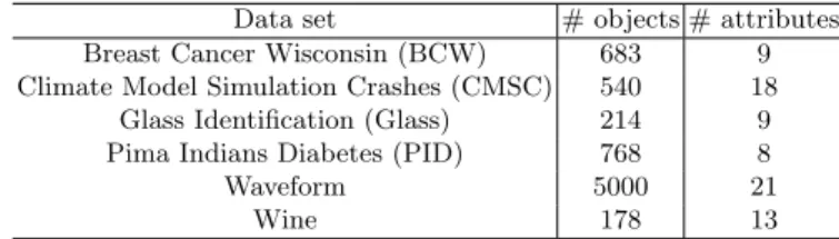
Table 1.Data set characteristics

Data set # objects # attributes

Breast Cancer Wisconsin (BCW) 683 9

Climate Model Simulation Crashes (CMSC) 540 18

Glass Identiﬁcation (Glass) 214 9

Pima Indians Diabetes (PID) 768 8

Waveform 5000 21

Wine 178 13

ﬁxed. The standard deviation expresses the variability of a set of data. For sub-spaceS, we setϵ= √ r· ∑ Di∈S (σ2 Di++σ 2 Di−) (r≥0), whereσ 2 Di+ andσ 2 Di− are

the marginal variances of O+ and O₋, respectively, on dimensionDi (Di∈S),

andris a system deﬁned parameter. Our experiments show thatrcan be set in the range of 0.3∼0.6, and is not sensitive.

5 Empirical Evaluation

In this section, we report a systematic empirical study using real data sets to verify the eﬀectiveness and eﬃciency of our method. All experiments were con-ducted on a PC computer with an Intel Core i7-3770 3.40 GHz CPU, and 8 GB main memory, running Windows 7 operating system. All algorithms were implemented in Java and compiled by JDK 7.

5.1 Eﬀectiveness

We use 6 real data sets from the UCI machine learning repository [18]. We remove non-numerical attributes and all instances containing missing values. Table 1 shows the data characteristics.

(11)

For each data set, we take each record as a query objectq, and all records exceptqbelonging to the same class asqforming the setO1, and records

belong-ing to the other classes formbelong-ing the setO2. Using CSMiner, we compute for each

record (1) theinlying contrast subspace takingO1asO+ andO2asO₋, and (2)

the outlying contrast subspace taking O2 as O+ and O1 as O₋. In this

experi-ment, we only compute the top-1 subspace. For clarity, we denote the likelihood contrasts of inlying contrast subspace byLCin

S (q) and those of outlying contrast

subspace byLCout

S (q). The minimum likelihood threshold is set to 0.001.

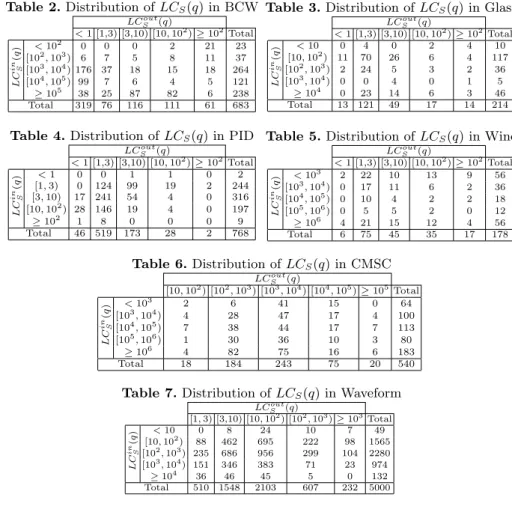
Tables 2∼7 list the joint distributions ofLCin

S (q) andLCSout(q) in each data

set. As expected, for most objectsLC_Sin(q) are larger than LC_Sout(q). However, interestingly a good portion of objects have strong outlying contrast subspaces. For example, in CMSC, more than 50% of the objects have outlying contrast subspaces satisfying LC_Sout(q) ≥ 103. Moreover, we can see that, except PID, a non-trivial number of objects in each data set have both strong inlying and outlying contrast subspaces (e.g.,LCin

S (q)≥10

4 _and_LCout

S (q)≥10

2_).

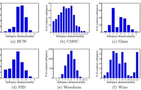
Figures 1, 2 show the distributions of dimensionality of inlying and outlying contrast subspaces, respectively. The dimensionality distribution is an interesting feature characterizing a data set. For example, in most cases the dimensionali-ty of contrast subspaces follows a two-side bell-shape distribution. However, in BCW and PID, the outlying contrast subspaces tend to have low dimensionality.

5.2 Eﬃciency

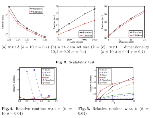
To the best of our knowledge, there is no previous method tackling the exact same mining problem. Therefore, we evaluate the eﬃciency of only CSMiner and the baseline method. Limited by space, we report the results on the Waveform data set only, since it is the largest one with the highest dimensionality. We randomly select 100 records from Waveform as query objects, and report the average runtime. The results on the other data sets follow similar trends.

Figure 3(a) shows the runtime (in logarithmic scale) with respect to the min-imum likelihood thresholdδ. Asδdecreases, the runtime increases exponentially. However, the heuristic pruning techniques in CSMiner expedites the search sub-stantially in practice. Figures 3(b) and 3(c) show the scalability on data set size and dimensionality. CSMiner is substantially faster than the baseline method.

CSMiner uses a user deﬁned parameterrto deﬁneϵ-neighborhood. Figure 4 shows the relative runtime with respect tor. The runtime of CSMiner is not very sensitive tor in general. Experimentally, the shortest runtime of CSMiner hap-pens whenris in [0.3,0.6]. Figure 5 illustrates the relative runtime of CSMiner with respect tok, showing that CSMiner is linearly scalable with respect tok.

6 Conclusions

In this paper, we studied a novel and interesting problem of mining contrast subspaces to discover the aspects that a query object most similar to a class and dissimilar to the other class. We showed theoretically that the problem

(12)

Table 2.Distribution ofLCS(q) in BCW LCout S (q) <1 [1,3) [3,10) [10,102₎_≥₁₀2_Total LC in S ( q ) <102 ₀ ₀ ₀ ₂ ₂₁ ₂₃ [102,103) 6 7 5 8 11 37 [103,104) 176 37 18 15 18 264 [104,105) 99 7 6 4 5 121 ≥105 38 25 87 82 6 238 Total 319 76 116 111 61 683

Table 3.Distribution ofLCS(q) in Glass

LCout S (q) <1 [1,3) [3,10) [10,102)≥102Total LC in S ( q ) <10 0 4 0 2 4 10 [10,102₎ ₁₁ ₇₀ ₂₆ ₆ ₄ ₁₁₇ [102_,₁₀3₎ ₂ ₂₄ ₅ ₃ ₂ ₃₆ [103_,₁₀4₎ ₀ ₀ ₄ ₀ ₁ ₅ ≥104 ₀ ₂₃ ₁₄ ₆ ₃ ₄₆ Total 13 121 49 17 14 214

Table 4.Distribution ofLCS(q) in PID

LCout S (q) <1 [1,3) [3,10) [10,102)≥102Total LC in S ( q ) <1 0 0 1 1 0 2 [1,3) 0 124 99 19 2 244 [3,10) 17 241 54 4 0 316 [10,102_{) 28} ₁₄₆ ₁₉ ₄ ₀ ₁₉₇ ≥102 ₁ ₈ ₀ ₀ ₀ ₉ Total 46 519 173 28 2 768

Table 5.Distribution ofLCS(q) in Wine

LCout S (q) <1 [1,3) [3,10) [10,102)≥102Total LC in S ( q ) <103 ₂ ₂₂ ₁₀ ₁₃ ₉ ₅₆ [103_,₁₀4₎ ₀ ₁₇ ₁₁ ₆ ₂ ₃₆ [104_,₁₀5₎ ₀ ₁₀ ₄ ₂ ₂ ₁₈ [105_,₁₀6₎ ₀ ₅ ₅ ₂ ₀ ₁₂ ≥106 ₄ ₂₁ ₁₅ ₁₂ ₄ ₅₆ Total 6 75 45 35 17 178 Table 6.Distribution ofLCS(q) in CMSC LCSout(q) [10,102_{) [10}2_,₁₀3_{) [10}3_,₁₀4_{) [10}4_,₁₀5₎_≥₁₀5_Total LC in S ( q ) <103 2 6 41 15 0 64 [103_,₁₀4₎ ₄ ₂₈ ₄₇ ₁₇ ₄ ₁₀₀ [104_,₁₀5₎ ₇ ₃₈ ₄₄ ₁₇ ₇ ₁₁₃ [105_,₁₀6₎ ₁ ₃₀ ₃₆ ₁₀ ₃ ₈₀ ≥106 ₄ ₈₂ ₇₅ ₁₆ ₆ ₁₈₃ Total 18 184 243 75 20 540

Table 7.Distribution ofLCS(q) in Waveform

LCout S (q) [1,3) [3,10) [10,102) [102,103)≥103Total LC in S ( q ) <10 0 8 24 10 7 49 [10,102₎ ₈₈ ₄₆₂ ₆₉₅ ₂₂₂ ₉₈ ₁₅₆₅ [102_,₁₀3_{) 235} ₆₈₆ ₉₅₆ ₂₉₉ ₁₀₄ ₂₂₈₀ [103,104) 151 346 383 71 23 974 ≥104 ₃₆ ₄₆ ₄₅ ₅ ₀ ₁₃₂ Total 510 1548 2103 607 232 5000

is very challenging, and cannot even be approximated in polynomial time. We presented a heuristic method based on upper and lower bounds of likelihood and likelihood contrast. Our experiments on real data sets clearly show that our method expedites contrast subspace mining substantially comparing to the baseline method.

References

1. Jeﬀreys, H.: The Theory of Probability. 3rd edn. Oxford (1961)

2. Dong, G., Bailey, J., eds.: Contrast Data Mining: Concepts, Algorithms, and Ap-plications. CRC Press (2013)

3. Dong, G., Li, J.: Eﬃcient mining of emerging patterns: discovering trends and diﬀerences. In KDD (1999) 43–52

4. Bay, S.D., Pazzani, M.J.: Detecting group diﬀerences: Mining contrast sets. Data Mining and Knowledge Discovery5(3) (2001) 213–246

(13)

1 2 3 4 5 6 7 8 0 50 100 150 200 250 Subspace dimensionality # of contrast subspaces (a) BCW 2 3 4 5 6 7 8 9 10 11 12 13 14 15 0 20 40 60 80 Subspace dimensionality # of contrast subspaces (b) CMSC 1 2 3 4 5 6 7 8 9 0 20 40 60 80 Subspace dimensionality # of contrast subspaces (c) Glass 1 2 3 4 5 6 7 8 0 50 100 150 200 250 Subspace dimensionality # of contrast subspaces (d) PID 1 2 3 4 5 6 7 8 9 10 11 0 500 1000 1500 Subspace dimensionality # of contrast subspaces (e) Waveform 2 3 4 5 6 7 8 9 10 11 12 13 0 5 10 15 20 25 30 Subspace dimensionality # of contrast subspaces (f) Wine

Fig. 1.Dimensionality distributions of inlying contrast subspaces

1 2 3 4 5 6 7 0 100 200 300 400 500 Subspace dimensionality # of contrast subspaces (a) BCW 2 6 7 8 9 10 11 12 13 14 15 0 50 100 150 Subspace dimensionality # of contrast subspaces (b) CMSC 1 2 3 4 5 6 7 8 0 20 40 60 80 100 Subspace dimensionality # of contrast subspaces (c) Glass 1 2 3 4 5 6 7 8 0 50 100 150 200 Subspace dimensionality # of contrast subspaces (d) PID 1 2 3 4 5 6 7 8 9 0 500 1000 1500 Subspace dimensionality # of contrast subspaces (e) Waveform 1 2 3 4 5 6 7 8 9 10 11 12 13 0 10 20 30 40 Subspace dimensionality # of contrast subspaces (f) Wine

Fig. 2.Dimensionality distributions of outlying contrast subspaces

5. Wrobel, S.: An algorithm for multi-relational discovery of subgroups. In PKDD (1997) 78–87

6. Novak, P.K., Lavrac, N., Webb, G.I.: Supervised descriptive rule discovery: A unifying survey of contrast set, emerging pattern and subgroup mining. Journal of Machine Learning Research10(2009) 377–403

(14)

0.01 0.04 0.07 0.1 0.13 100 101 δ Runtime (sec) Baseline CSMiner (a) w.r.tδ(k= 10, r= 0.4) 15005 2500 4000 5000 10 15 20 25 30

Data set size

Runtime (sec)

Baseline CSMiner

(b) w.r.t data set size (k = 10, δ= 0.01, r= 0.4) 5 10 15 21 10−2 10−1 100 101 102 Dimensionality Runtime (sec) Baseline CSMiner (c) w.r.t dimensionality (k= 10, δ= 0.01, r= 0.4)

Fig. 3.Scalability test

0.2 0.3 0.4 0.5 0.6 0.7 1 1.05 1.1 1.15 r Relative runtime BCW CMSC Glass PID Waveform Wine

Fig. 4. Relative runtime w.r.t r (k =

10, δ= 0.01) 10 20 50 100 1 1.02 1.04 1.06 1.08 1.1 k Relative runtime BCW CMSC Glass PID Waveform Wine

Fig. 5. Relative runtime w.r.t k (δ =

0.01)

7. Nguyen, H.V., M¨uller, E., Vreeken, J.,et al.: CMI: An information-theoretic con-trast measure for enhancing subspace cluster and outlier detection. In SDM (2013) 198–206

8. Keller, F., M¨uller, E., B¨ohm, K.: HiCS: High contrast subspaces for density-based outlier ranking. In ICDE (2012) 1037–1048

9. Breunig, M.M., Kriegel, H.P., Ng, R.T., Sander, J.: LOF: identifying density-based local outliers. In SIGMOD (2000) 93–104

10. Kriegel, H.P., S hubert, M., Zimek, A.: Angle-based outlier detection in high-dimensional data. In KDD (2008) 444–452

11. He, Z., Xu, X., Huang, Z.J., Deng, S.: FP-outlier: Frequent pattern based outlier detection. Computer Science and Information Systems2(1) (2005) 103–118 12. Aggarwal, C.C., Yu, P.S.: Outlier detection for high dimensional data. In: ACM

Sigmod Record. Volume 30. (2001) 37–46

13. Hua, M., Pei, J., Fu, A.W., et al.: Top-k typicality queries and eﬃcient query answering methods on large databases. The VLDB Journal18(3) (2009) 809–835 14. Breiman, L., Meisel, W., Purcell, E.: Variable kernel estimates of multivariate

densities. Technometrics19(2) (1977) 135–144

15. Silverman, B.W.: Density Estimation for Statistics and Data Analysis. Chapman and Hall/CRC, London (1986)

16. Wang, L., Zhao, H., Dong, G., Li, J.: On the complexity of ﬁnding emerging patterns. Theor. Comput. Sci.335(1) (2005) 15–27

17. Rymon, R.: Search through systematic set enumeration. In: Proc. of the 3rd Int’l Conf. on Principles of Knowledge Representation and Reasoning. (1992) 539–550 18. Bache, K., Lichman, M.: UCI machine learning repository (2013)