How Sensitive Are Taxpayers to Marginal Tax Rates?
Evidence from Income Bunching in the United States
Jacob A. Mortenson
*and Andrew Whitten
*October 1, 2015
Abstract
Understanding the way taxpayers respond to the tax code is critical for revenue and welfare analyses of taxation. One way taxpayers may respond is by bunching at kink points in the tax schedule to avoid higher marginal tax rates. We study this phe-nomenon using over 100 million federal individual income tax returns in the United States from 1996 to 2011, analyzing state and federal statutory kinks as well as effec-tive kinks created by income phase-outs for tax credits. Though many kinks do not cause statistically discernible bunching, we find growing responsiveness at other kinks. Consistent with prior research, we find increasingly strong bunching patterns at the first kink of the Earned Income Tax Credit (EITC) schedule over time. In addition, we present new evidence documenting the emergence and rapid rise of bunching at the second EITC kink and the Child Tax Credit refundability plateau. We also observe a small, steady bunching response at the largest kink in the federal ordinary income tax schedule. When translating bunching patterns to elasticities of taxable income, we find a range of values from zero to 1.59, with substantial variation by observable characteristics such as age, gender, and self-employment status. Finally, we uncover a few bunching puzzles: consistent bunching at seemingly uneventful locations in the income distribution.
Keywords: Bunching, Elasticity of Taxable Income, Public Finance.
JEL Code: H24.
*Both authors: Georgetown University and Congressional Joint Committee on Taxation. Contact email:
[email protected]. This research embodies work undertaken for the staff of the Joint Committee on Taxation, but as members of both parties and both houses of Congress comprise the Joint Committee on Taxation, this work should not be construed to represent the position of any member of the Committee.
1
Introduction
This paper estimates taxpayer responsiveness to marginal income tax rates by measuring the degree to which taxpayers bunch at kink points in income tax schedules. A kink point is an income amount for a given taxpayer at which marginal tax rates change discretely, marking the end of one tax bracket and the beginning of the next.1 Standard economic
theory predicts that households will bunch at kink points where tax rates increase, creating extra mass in the distribution of income close to the kink. We use measures of bunching to estimate elasticities of taxable income (ETIs) following Saez (2010).
ETIs are necessary statistics for performing welfare and revenue analyses of current and proposed income tax policies (Chetty, 2009). They capture the degree to which taxable income responds to its marginal tax rate, and allow for responses through labor supply, deduction, and evasion decisions. Understanding how ETIs vary across household types is also important. The federal income tax code in the U.S. is vast and complex. Many policies affect subpopulations differently, reducing the usefulness of population-level average treatment effects. In this paper, we estimate ETIs at a finer grain than previous research, reporting estimates annually and allowing for variation by household type, income level, and tax year. We are the first to report elasticities with this scope of heterogeneity.
The conventional method of estimating ETIs is a reduced form regression of tax bases (e.g. taxable income) on their net-of-tax rates (one minus the marginal tax rate) and other controls. Identification of a treatment effect using this approach relies on cross-sectional and time series variation in tax rates. Several issues pose major problems for this strategy. The most critical is endogeneity of marginal income tax rates, which arises mechanically when tax rates are a function of income, as is the case in virtually every income tax system in the world. Other serious impediments to identification include mean reversion in the dependent variable (income), heterogeneous secular income trends, and changes in the definition of taxable income over time. Various methods have been employed to address these problems, and substantial progress has been made, but the literature has thus far failed to converge on consensus estimates for ETIs.2
The bunching approach, on the other hand, does not rely on cross-sectional or time series variation in tax rates, and is not subject to any of the problems mentioned above. Identification comes directly from changes in tax rates inherent to the structure of the tax code—precisely the mechanical endogeneity of tax rates that plagues the regression approach. These tax rate changes are within-year and within-household, allowing us to address ques-tions on which the conventional method is mute (e.g. “How does taxpayer sensitivity change
1See Moffitt (1990) on the “econometrics of kinked budget constraints.”
2Saez et al. (2012) provide a good discussion of many of these issues. For thorough treatment of the
from year to year?”).
We measure bunching using detailed administrative data drawn from the universe of federal income tax returns in the United States from 1996 to 2011. Most of our estimators – including those for narrowly defined household types – use tens or hundreds of thousands of observations, resulting in smooth distributions over the intervals surrounding kinks. We build upon work by Saez (2010) and Chetty et al. (2011) in generating ETI estimates, and our bunching results associated with the Earned Income Tax Credit (EITC) are broadly consistent with Saez’s. However, Saez measures bunching using public-use data through 2004, while our dataset – which is significantly larger and more recent – allows us to make a series of improvements to bunching and income measures.
We make four contributions to the modern public finance literature estimating sensitivity to marginal tax rates. First, we allow for heterogeneous income responses across household types to the U.S. federal income tax code. Second, we measureannual variation in tax rate sensitivity over a sixteen-year period that includes the Bush Tax Cuts and several business cycle fluctuations, including the Great Recession. Third, unlike prior literature, we derive the bunching estimator of Saez (2010) without imposing a functional form on utility. Fourth, we employ an estimation technique that fits more closely with the theory of discrete kinks and show how our technique compares with those of Saez (2010) and Chetty et al. (2011).
Our primary finding is a striking absence of responsiveness at most kinks, including most convex kinks (where marginal tax rates rise) that affect middle and high income earners, and all non-convex kinks (where marginal tax rates fall). However, there are important exceptions at convex kinks towards to bottom of the income distribution. Consistent with Saez (2010) and Chetty et al. (2013), we find sharp bunching at the first kink in the EITC schedule. The strongest results are for self-employed taxpayers with one child. For these households we calculate observed elasticities of up to 1.59.
We also present a number of novel findings. First, we find statistically significant and economically meaningful bunching patterns at the second EITC kink beginning in the mid 2000s. Second, we find bunching among married taxpayers at the second kink in the federal statutory marginal tax rate schedule (transitioning from a 15% rate to a 25% rate). This holds for both wage earners and the self-employed, though wage earners may be more re-sponsive at this kink. Third, we document substantial bunching at the kink in the Child Tax Credit (CTC) schedule at which the credit is fully refundable. Finally, we document visually evident, statistically significant bunching among wage earners at each of the kinks where the self-employed bunch – the first evidence of wage-earner bunching in the U.S.
The bunching patterns we observe, and the corresponding elasticity estimates, are evolv-ing over time. At the first EITC kink, bunchevolv-ing patterns grow over time for some groups. At the second EITC kink and the CTC refundability plateau, bunching is nonexistent in the
late 1990s and early 2000s, but emerges in the mid 2000s and increases through the end of our sample, 2011. In addition, the most responsive groups at the first EITC kink exhibit patterns that suggest bunching is positively correlated with business cycles. The Great Re-cession drastically reduced bunching for these groups, though subsequent years saw a return to pre-recession bunching levels.
Our findings have several policy implications. Primarily, they speak to the importance of thinking carefully about the structure of the tax code. Many tax credits, including the EITC, introduce large kinks into the effective tax schedule. These kinks distort income earning decisions, and our results indicate these distortions are growing over time. The emergence of bunching at the second EITC kink, in particular, suggests taxpayers have learned more about the EITC’s structure. This increased responsiveness at the beginning of the credit’s phaseout region – which induces negative substitution and income effects – works against the credit’s intended effect of encouraging work. Policymakers should consider altering the structure of the credit in order to minimize this effect. In addition, our results suggest ETIs may fall during recessions. Thus counter-cyclical tax cuts may be less effective at increasing labor supply than policymakers anticipate. We also provide clear evidence of income adjustments in response to the CTC. The associated welfare loss could be avoided if the credit were fully refundable for all low-income taxpayers.
2
Bunching Theory
Why should we expect taxpayers to bunch at kink points? In this section, we show that this behavioral response is a straightforward implication of a positive elasticity of taxable income (ETI). We assume throughout that taxpayers are fully aware of the tax schedule and that they manipulate earnings with arbitrary precision. These assumptions are unlikely to hold in practice but are useful for characterizing a frictionless response to taxation. When estimating elasticities in Section 7, we discuss the relationship between our elasticity estimates and the structural elasticities described here. Let 𝑒 ≡ 𝑑𝑧
𝑑(1−𝑡) 1−𝑡
𝑧 denote the elasticity of taxable
income (𝑧) with respect to the net-of-tax rate (1 −𝑡), where 𝑡 denotes the marginal tax rate.3 Suppose this elasticity is constant in a neighborhood around kink point 𝑧*. Under this assumption, and using the definition of the ETI, we solve the differential equation
𝑒· 𝑑(11−−𝑡𝑡) = 𝑑𝑧𝑧. The result is that income takes the functional form
𝑧 =𝑛·(1−𝑡)𝑒 (1)
locally around kink𝑧* for some𝑛, which we call potential income.4 This solution is identical 3Technically,𝑒is the uncompensated elasticity of taxable income. In the absence of income effects, it can
to that which emerges from the structural assumptions of Saez (2010). In that setting, agents also choose taxable income according to equation (1), but this comes from maximizing a quasi-linear, iso-elastic utility function under a standard budget constraint. Here we have shown that the only assumption embedded in the structural approach necessary for income to take this functional form is a constant elasticity in the neighborhood of the kink. The rest of the trappings of the structural approach are superfluous (and therefore benign).5
With our empirical approach in mind, we now assume all earners face the same local tax schedule and have the same elasticity, 𝑒 > 0.6 In this case, the only parameter that creates dispersion in income is potential income (𝑛), which we take to be distributed according to a smooth, atomless density 𝑓(·), with distribution function 𝐹(·).
Suppose that the marginal tax rate is𝑡0 up to kink𝑧*, and𝑡1 thereafter. Here we analyze
convex kinks, such that 𝑡0 < 𝑡1. In this case, the space of potential income can be divided
into three regions. Those with low potential income choose income below the kink; those with high potential income choose income above the kink; and those with moderate potential income locate precisely at the kink. Specifically, define 𝑛𝑗 ≡𝑧*/(1−𝑡𝑗)𝑒 for 𝑗 = 0,1. Then
𝑧 =𝑛·(1−𝑡0)𝑒 for 𝑛 ≤𝑛0 and 𝑧 =𝑛·(1−𝑡1)𝑒 for 𝑛 ≥𝑛1. The remaining mass of earners
with 𝑛∈(𝑛0, 𝑛1) are unable to achieve their desired solution according to (1). When facing
rate 𝑡0, they desire income greater than 𝑧*, but when facing rate 𝑡1, they want less income
than 𝑧*. Consequently, they bunch precisely at the kink (i.e. 𝑧 = 𝑧*). Their mass is given by7 𝐵 ≡ ∫︁ 𝑛1 𝑛0 𝑓(𝑛)𝑑𝑛≈(𝑛1−𝑛0) 𝑓(𝑛0) +𝑓(𝑛1) 2 . (2)
Here we have derived an expression for the mass of bunchers assuming all taxpayers share the same elasticity. This will be useful later when we translate bunching patterns to elasticity estimates. However, homogeneity in elasticities is not needed to imply the existence of a bunching response. Bunching would arise under heterogeneous elasticities provided they are positive and locally constant, assuming taxpayers respond frictionlessly to fully salient tax schedules.8
5In addition to yielding solution (1), the structural approach assumes away income effects and therefore
assigns𝑒the dual roles of the compensated and uncompensated ETI. As there is some evidence of trivially small income effects (Gruber and Saez, 2002; Bastani and Selin, 2014), we follow the structural approach in interpreting our estimates for ETIs as compensated elasticities.
6Though the constant elasticity assumption is ubiquitous in the literature estimating ETIs, our evidence
indicates it is unlikely to hold when estimating population parameters. It is more plausible in our case, as we merely assume the elasticity is locally constant around each kink for a given household type in a given year.
7Note that if potential income has a linear distribution function (e.g. if it is distributed uniformly) then
Equation (2) holds with precise equality.
8Bunching can arise under imperfect optimization as well. We merely need some fraction of taxpayers to
As it stands, equation (2) is not estimable because we do not observe the distribution of potential income. However, we can relate the distribution of potential income with the observed distributions of income under marginal tax rates 𝑡0 and 𝑡1, respectively. Let 𝐻𝑗
denote the distribution function and ℎ𝑗 the density over income that would arise if the tax
rate were 𝑡𝑗 both above and below the kink. From equation (1), 𝐻𝑗(𝑧) =𝐹(𝑧/(1−𝑡𝑗)𝑒), so
that ℎ𝑗(𝑧) =𝑓(𝑧/(1−𝑡𝑗)𝑒)/(1−𝑡𝑗)𝑒. This implies 𝑓(𝑛𝑗) =ℎ𝑗(𝑧*)·(1−𝑡𝑗)𝑒. Applying this
result to equation (2), with a bit of algebraic manipulation, gives
𝐵 ≈ 𝑧 * 2 (︂ ℎ0(𝑧*) [︂(︂ 1−𝑡0 1−𝑡1 )︂𝑒 −1 ]︂ +ℎ1(𝑧*) [︂ 1− (︂ 1−𝑡1 1−𝑡0 )︂𝑒]︂)︂ , (3)
which allows us to translate bunching patterns to observed elasticities. Tax rates 𝑡0, 𝑡1, and
kink point 𝑧* are directly observable in the tax code. Thus, we can identify an estimate for
𝑒 given estimates for parameters 𝐵, ℎ0(𝑧*), and ℎ1(𝑧*). We estimate these using predicted
counterfactual distributions, as described in detail in Section 6.2. Intuitively, if we step far enough away from the kink, the distribution of income will no longer be affected by bunching behavior. Instead, it will reflect the distribution of income under a constant marginal tax rate. Thus, we can use the actual distribution of income far from the kink to inform the
counterfactual distribution of income that would obtain near the kink if the tax rate did not change.
3
Existing Estimates of Responses to Income Taxation
In this section we review existing estimates of responses to income taxation. There are four main approaches to estimating tax rate sensitivity: difference-in-difference analysis (the conventional approach), bunching analysis, share analysis, and nonlinear budget set analysis. We briefly review the first two branches of the literature here. Blomquist et al. (2014) discuss, illustrate, and extend the nonlinear budget set approach. For an example of the share analysis approach, see Romer and Romer (2014).
3.1
Difference-in-Difference Analyses
The most common method for estimating tax rate sensitivity analyzes panels of individual income tax returns, and uses tax reforms as quasi-natural experiments. These papers then estimate the responsiveness of changes in income over multi-year periods (to control for individual fixed effects) to changes in the net-of-tax rate.9 The mechanical endogeneity that
results from marginal tax rates being functions of income is addressed using instrumental
variables, typically constructed holding income constant at base year levels. This instrument only contains changes in tax rates associated with changes in marginal tax rate schedules.
Saez et al. (2012) review this literature, finding responses ranging from 0.1 to 0.4. How-ever, virtually every panel data study they review constructs instruments that fail a necessary condition for valid instruments: exogeneity. Weber (2014b) demonstrates that instruments constructed in the standard approach – holding income constant at base year levels – are endogenous because shocks to base year income are a component of the error term in the first and second stages.
Weber (2014b) proposes a set of instruments constructed using lagged income sufficiently far before the base year so that serially correlated shocks do not introduce a large bias. Four papers have used these instruments to estimate ETIs associated with three different sets of tax reforms in the United States. Weber (2014b) analyzes the Tax Reform Act of 1986 (TRA86), and estimates an elasticity of taxable income of around 0.9. Weber (2014a) also analyzes TRA86, but instead estimates an intent-to-treat effect. This estimate is slightly larger and more precise than the average treatment effect estimated in Weber (2014b). Auten and Kawano (2013) find large responses associated with the Omnibus Budget Reconciliation Act of 1993 (many of their ETI estimates are greater than unity), but also find some evidence of inter-temporal income shifting. Finally, Mortenson (2015) analyzes the Bush Tax Cuts of 2001 and 2003, finding an elasticity of taxable income indistinguishable from zero.10
A major shortcoming of the panel data literature is an inability to analyze the responsive-ness of sub-populations. Variation in the “treatment” variable – the change in the net-of-tax rate – is necessary for identifying the average treatment effect or intent-to-treat effect using the panel data approach, and focusing on sub-populations substantially reduces this vari-ation. Further, this literature relies on large tax reforms to generate identifying variation, and these typically occur only once or twice a decade. This is problematic both because re-forms alter the definition of income (the dependent variable) and because compliance norms or enforcement practices might change over time, rendering distant estimates as historical artifacts, rather than contemporaneously relevant parameters.
3.2
Bunching Analyses
Analysis of taxpayer bunching began three decades ago with Slemrod (1985), studying tax evasion in the United States. He shows that taxpayers who under-report income have an incentive to report income near the top of $50 micro-brackets in the tax code. Using data
10Mortenson makes the broader point that the elasticity of taxable income is actually an elasticity of
ordinary income, as short and long-term capital gains are excluded from all ETI analyses. He then estimates cross-tax effects between ordinary income and long-term capital gains, finding evidence suggestive of shifting between these two bases.
from 1977, he finds excess mass of about 1-4% of households in the top quintile of these micro-brackets. MaCurdy et al. (1990) investigate bunching in hours worked associated with kink points and find none (though their data only contain 1,000 observations, resulting in low statistical power). Friedberg (2000) measures bunching associated with the earnings test for Social Security beneficiaries. She finds large responses, and estimates income and substitution effects that indicate the earnings test creates large dead-weight loss.11
To our knowledge, taxpayer bunching was ignored following Friedberg (2000) until the groundbreaking work of Saez (2010). Using a simple model, Saez maps a one-to-one rela-tionship between bunching levels and observed ETIs.12 Using public-use tax data from 1960-2004, he looks for bunching around kink points in the Earned Income Tax Credit (EITC) schedule and the federal income tax schedule. He finds substantial bunching only around the first EITC kink and at $0 of taxable income.13 These yield observed elasticities for the general population of approximately 0.10–0.33 and 0.11–0.26, respectively. All other kinks appear to generate no bunching, and yield observed elasticities that are statistically indis-tinguishable from zero. Importantly, when looking closer at the observed elasticities around the EITC schedule, Saez finds the response is driven entirely by the self-employed. Once they are removed from the sample, observed elasticities fall to 0.00–0.03 and are statistically insignificant. Isolating the self-employed yields observed elasticities of 0.75–1.10.
Following Saez (2010), a number of other studies have examined individual taxpayer bunching outside of the United States.14 Le Maire and Schjerning (2013) develop a two-period extension of the Saez model. Using taxpayer data in Denmark, they document evi-dence of intertemporal shifting of income. They find that more than half of observed bunch-ing patterns in a given year reflect intertemporal shiftbunch-ing. Once this is taken into account they calculate structural elasticities of around 0.14–0.20. Chetty et al. (2011) also study taxpayer bunching in Denmark. They distinguish between micro and macro ETIs, where the latter reflect changes in the aggregate labor market in response to tax code changes. They find convincing evidence of bunching, but these patterns translate to observed elasticities no greater than 0.02.
11Gelber et al. (2013) build on the work of Friedberg (2000) and estimate bunching associated with the
Social Security Earnings Test. They estimate an earnings elasticity with respect to the net-of-tax rate of 0.23 and simultaneously estimate adjustment costs of approximately $150.
12Saez (2010) does not distinguish observed and structural ETIs, but we retain our preferred nomenclature
in this section for consistency with the rest of the paper. See Section 7 for definitions and discussion of “observed” and “structural” elasticities.
13The first EITC kink sees the marginal subsidy rate change from 7.65-40% (depending on tax year and
number of dependents) to 0%. In most of the years Saez studies, the kink at $0 of taxable income sees the marginal tax rate increase from 0% to 14-16%.
14Devereux et al. (2014) estimate an elasticity of corporate taxable income in the United Kingdom by
measuring bunching at corporate marginal tax rate kinks. They find that closely held corporations bunch to a higher degree than widely held corporations.
Bastani and Selin (2014) study taxpayer bunching at a large kink in Sweden, calculating an observed elasticity of precisely zero. From this they calculate an upper bound on the structural elasticity of 0.39 in the context of optimization frictions, using the methods of Chetty (2012). This upper bound is tighter than that found by Chetty, who pools the results of fifteen other papers in the literature, showing they are all consistent with a single structural elasticity as high as 0.54.
Kleven and Waseem (2013) study taxpayer bunching around tax notches in Pakistan. Notches are more severe versions of kinks where average tax rates change discretely, pro-ducing a discontinuity in the budget set. In progressive schedules, such as in Pakistan, this creates dominated regions in the income distribution where no taxpayer should locate.15 However, many taxpayersdo locate in dominated regions, providing strong evidence of opti-mization frictions. After accounting for frictions, the authors calculate structural elasticities around most kinks in the range of 0.02-0.25. Consistent with the findings of Saez (2010), the results are driven by the self-employed. Once they are removed from the sample, structural elasticities lie in the range 0.00-0.07.
4
Data
We analyze taxpayer bunching using data drawn from the Internal Revenue Service’s Com-pliance Data Warehouse (CDW). The CDW contains the universe of individual tax returns (e.g. Form 1040 and its schedules) and information returns (e.g. Form W-2) of individuals in the United States. Each observation in the data is a tax unit that filed a tax return for a given year. This could be an individual or a married couple filing jointly. Most of the data consist of fields on the tax return and its schedules. These include ordinary and capital gains income, as well as deductions, credits, and taxes paid. Certain demographic information is also found on tax returns, such as marital status, number of children, years of birth of those in the tax unit, and state of residence. We also make use of information from the Form W-2 and the Social Security Administration’s Data Master File, which includes industry of employment, date of death, and sex at the time of birth.
Our primary set of data is a sample from the CDW consisting of all tax returns in the seven states with no state income taxes: Alaska, Florida, Nevada, South Dakota, Texas, Washington, and Wyoming. We choose this subsample for two reasons. First, and most important, state income tax regimes can create new kinks. These kinks may be close to the kinks we study, complicating the analysis substantially. Similarly, many states have
15A Pakistani taxpayer in a dominated region could earn less pre-tax income, pay a lower average tax
rate, and take home more after-tax income. This is impossible at the simple kinks we study, as changes in
their own earned income tax credits, often amplifying the existing federal credit. Including observations from these states but ignoring state-specific taxes and subsidies – as done in Saez (2010) – introduces bias into elasticity estimates. We avoid this as the states in our sample do not have active earned income credits during our period of analysis.16 Second,
this sample significantly reduces computation time while still affording a sufficient number of observations to identify heterogeneous responses in narrow subpopulations.
We also draw several subsamples for specific kinks. One is a sample from the CDW consisting of all tax returns in the United States in the neighborhood of kinks created by phaseouts of personal exemptions and itemized deductions. The mass from the seven states with no income tax regimes was insufficient to analyze these kinks. Another data set is a sample from the CDW consisting of all tax returns in certain states in the neighborhood of certain state income tax kink points. We examined the largest kinks in California, Connecti-cut, and New Jersey from 2003 to 2011.
Our data cover the years 1996 to 2011. This allows us to estimate how bunching patterns and their corresponding observed elasticities vary from year-to-year, the first such analysis of its kind. The period also allows us to see how tax rate sensitivity was affected by the Bush Tax Cuts and several business cycle fluctuations, including the Great Recession.
5
Institutional Background
In this section we briefly describe the portions of the U.S. tax code we study. We begin with an overview of the statutory federal schedule. This is followed by discussions of personal exemption and itemized deduction phase-outs, as well as the Earned Income Tax Credit and the Child Tax Credit.
5.1
Federal Tax Code
Despite its well deserved reputation for complexity, the U.S. federal income tax code has a straightforward statutory schedule.17 In 1996, the first year in our sample, the schedule for ordinary income had five tax brackets whose marginal tax rates are detailed in Table 1.18 This schedule remained stable, on an inflation-adjusted basis, until the Bush Tax Cuts
16Washington enacted its earned income credit, the Washington Working Families Credit, in 2008, but it
has yet to fund and implement the credit.
17The complexity comes from the many rules that govern the definition of “taxable income,” as well as
myriad credits and deductions.
18The actual implementation of Table 1’s marginal tax rates involves a large number of $50 micro-brackets,
with discrete changes in tax liability only at the beginning of each bracket. Hence, the effective tax rate on marginal income is actually zero for most taxpayers for small enough marginal income increments. Like most other researchers, we ignore this, sticking with the simpler approximation of the tax code given by the
Table 1: Federal ordinary income tax: Statutory marginal tax rates (%) Bracket Year(s) 1st 2nd 3rd 4th 5th 6th 1996-2000 — 15 28 31 36 39.6 2001 — 15 27.5 30.5 35.5 39.1 2002 10 15 27 30 35 38.6 2003-2011 10 15 25 28 33 35
of 2001-2003, which added a 10% bracket at the beginning of the schedule and generally lowered rates.19 The Bush tax rates remained in place for the remainder of our sample period, although they were altered by the American Taxpayer Relief Act of 2012.
The kink points separating the federal tax brackets vary by year and by filing status. Throughout the paper we take the “first” kink to be the divider between the first and second brackets. Similarly, we take the “second” kink to be the divider between the second and third brackets, and so on. Thus, in our terminology, the first kink did not exist in 1996-2001. The “zeroth” kink marks the beginning of the schedule in all years.
Unlike the EITC and CTC schedules, the federal income tax schedule is progressive. All kinks see marginal tax rates increase and are therefore convex. The statutory marginal tax rate schedule applies to taxable income, which is adjusted gross income (AGI) minus the sum of exemptions and the larger of the standard deduction and itemized deductions. Adjusted gross income is total income less above-the-line deductions, both of which are calculated on the front page of the Form 1040. Exemptions are calculated by summing the number of people on the tax return and multiplying them by a fixed “per exemption” amount, $3,700 in 2011. The standard deduction is a function of the filing status of the return (e.g. single, married, or married filing separately) and the age of the primary and secondary filers on the return. In 2011, the standard deduction for a married-filing-jointly return with primary and secondary filers under 65 years of age was $11,600. Itemized deductions are listed on Schedule A of Form 1040 and include charitable gifts, mortgage interest, and some medical expenses, among other items.
5.2
Personal Exemption and Itemized Deduction Phase-outs
Personal exemptions and itemized deductions phase-out at high income levels, creating dis-continuities in the budget constraints of high income taxpayers. These phase-outs were in effect during our sample from 1996 to 2005, but were gradually removed beginning in 2006,
19Following convention, we refer to the Economic Growth and Tax Relief Reconciliation Act of 2001 and
with full removal from 2010 to 2012. They have since been reinstated.
The personal exemption phase-out (PEP) is a step function of AGI, generating notches in the budget constraint. Personal exemptions are reduced by 2% for each $2,500 of income exceeding the phase-out threshold until exemptions are exhausted. The beginning (and end) of the phase-out varies by filing status: $145,950 for singles, $182,450 for head of household, and $218,950 for married couples filing jointly in 2005.20
The itemized deduction phase-out (Pease) reduces certain itemized deductions at a rate of 3 cents per dollar of AGI exceeding the threshold. However, Pease (named after former Ohio Congressman Donald Pease) does not apply against itemized deductions generated from casualty and theft losses, investment interest, gambling losses, or medical expenses. Also, the total percentage of itemized deductions eliminated by Pease is capped at 80% per taxpayer. The threshold for Pease throughout the time period we study (1996-2005) is the same for all filing statuses except married couples filing separately, for whom the threshold is halved. In 2005 the threshold was $145,950 ($72,975), identical to the PEP threshold for singles.
Pease creates relatively small changes in marginal tax rates at its introduction and conclu-sion. For example, suppose a head of household with three children claims $20,000 of itemized deductions and earns exactly the Pease threshold of $145,950 in 2005. For a marginal in-crease of $1,000 above the Pease threshold, qualified itemized deductions are reduced by by 3%, meaning the individual has 30 additional dollars of taxable income. If the taxpayer faces an initial marginal tax rate of 31%, she would see her marginal rate increase by around 1 percentage point ($30×31%/$1000) as a result of Pease, which creates a small convex kink. Similarly, once Pease is phased out the change is also around 1 percentage point, which creates a small non-convex kink. In the presence of moderate optimization frictions, these kinks are unlikely to induce a behavioral response.
PEP generates larger marginal tax rate increases, but, because it is a notch, its size depends upon the magnitude of the marginal increment to income. Suppose the same tax-payer earns income at the PEP threshold. She has four personal exemptions, which reduce taxable income by 4×$3,200 = $12,800. If this taxpayer earns at least 1 additional dol-lar but less than 2,500 additional doldol-lars, her personal exemptions will be reduced by $256 (2% ×$12,800). Assuming her marginal tax rate is 31% initially, this increases her tax liability by 31%×$256 = $79.36. The implicit change in marginal tax rates in this case is 7,936 percentage points. If instead she increases her income by $1,000, the implicit change in marginal tax rates is 7.936 percentage points. In the analysis below, we take the most conservative measure, assuming the income increment is the full $2,500. Thus we take this
taxpayer’s kink size to be 3.17 percentage points.21
5.3
Earned Income Tax Credit
The EITC is one of the largest poverty alleviation policies (and tax expenditures) in the United States, with some 28 million low-income households receiving 63 billion dollars in 2011.22 These figures represent substantial growth in the past decade, as the dollar amount
in 2011 represents a nearly 100% increase in nominal dollars compared to 1999, when roughly 19.3 million households received $32 billion.23 All low-income taxpayers between the ages of
25 and 64 are eligible, and the age restriction only applies to taxpayers with no qualifying children.
The credit’s schedule varies based on filing status (single or married), number of qualifying children, and tax year. Childless households may qualify for a small credit (a maximum of $464 in 2011), but the EITC is much more generous for households with children. For example, a taxpayer with three qualifying children in 2011 could potentially take a credit up to $5,751.
The term “earned” in the credit’s title refers to the credit’s intended effect of increasing labor force participation. As earned income increases from zero, all households face a phase-in region, a plateau, and a phase-out region. In the phase-phase-in region, additional earned income is subsidized at rates between 7.65% and 45% depending on the number of qualifying dependents in the household. In the plateau region, the taxpayer receives the maximum credit amount, between $464 and $5,751 in 2011. Each additional dollar of qualifying income does not affect the credit amount. In the phase-out region, the subsidy is removed at rates between 7.65% and 21.06%, again depending on the number of qualifying dependents. This increases effective tax rates in this region, potentially discouraging earnings.24
Assuming a positive elasticity of taxable income, the credit should increase labor force participation, but its net effect on hours of work (and taxable income) is ambiguous. Those in the phase-in region will work more, but those in the phase-out region will work less.
We expect individuals to bunch around the first and second kinks, marking the beginning and end of the plateau region. Because it is non-convex, the kink at the end of the phase-out region should induce an absence of mass. In a frictionless environment, this would appear as a hole in the distribution of income, where no taxpayers locate. With moderate frictions,
21The formula for kink size, given an income increment of𝑋 ≤2500, is ((79.36/𝑋)×100%). 22See Eissa and Hoynes (2011) for an overview on the EITC.
23These figures are taken from the Statistic of Income’s “Tax Stats” website, specifically the section on
the EITC here: http://www.irs.gov/Individuals/Earned-Income-Tax-Credit-Statistics.
24Phaseout of the EITC occurs using the greater of earned income and AGI. In our empirical analysis
we ignore this issue, assuming all taxpayers have weakly greater earned income than AGI. Our measures, therefore, likely understate tax responsiveness at the second EITC kink.
it would more closely resemble a ditch.
5.4
Child Tax Credit
The Child Tax Credit (CTC) is available to taxpayers on a per child basis but phases out for those above certain income thresholds. The credit amount and refundability parameters have varied since the credit’s introduction in 1997. Initially the CTC was $400 per qualifying child. In 1999 it increased to $500; in 2001 and 2002 the credit was $600; and in 2003 the credit increased to its present value of $1,000 per qualifying child.25
The credit creates two convex and two non-convex kinks. The first non-convex kink is the refundability threshold, which was introduced in 2001. At this threshold the portion of the credit exceeding the taxpayer’s liability can be claimed by the individual, but only at a rate of 10% or 15% of earned income exceeding the threshold, depending on the year. This has no effect on households whose tax liability exceeds the credit amount. For the remaining households, however, the kink effectively decreases marginal tax rates by 10% or 15%. The threshold was $10,000 from 2001 to 2007 (indexed to inflation beginning in 2002), reduced in 2008 to $8,500, and reduced again in 2009 to $3,000 (not adjusted for inflation). The refundability rate was 10% from 2001 to 2003 and 15% after.
The first convex kink occurs at the point where the CTC has been fully refunded. After this point the credit is fully maximized, creating a plateau region. This ”refundability plateau kink” is comparable to the first EITC kink – the only kink we analyze where others have found bunching. A priori, this is the most likely place to find a bunching response to the CTC.
The second convex kink is at the end of the credit’s plateau and the beginning of the phase-out region, which is $75,000 for singles and $110,000 for married filing jointly (neither are indexed to inflation). The credit is reduced by $50 for every $1,000 in additional modified AGI, effectively increasing marginal tax rates by five percentage points. The end of the phase-out region – where the credit amount is completely eliminated – marks the second non-convex kink. At this point the taxpayer’s marginal tax rate decreases ceteris paribus. In a frictionless world, we would expect an absence of mass at this point. However, given that marginal tax rates change by only five percentage points, we do not expect to find responsiveness at either the beginning or end of the CTC phaseout region.
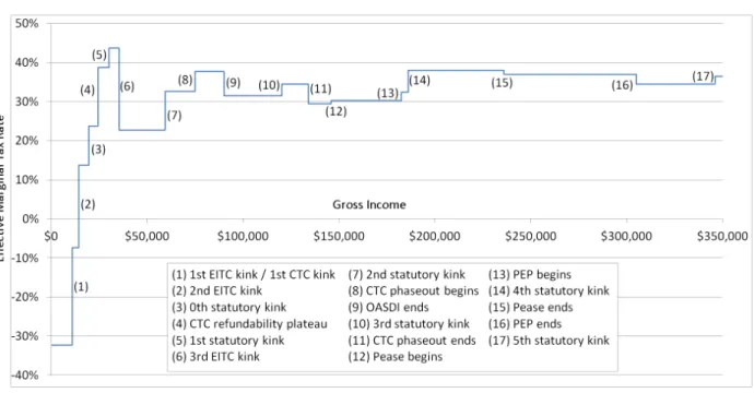
Figure 1: Kinks faced by a single parent with two children in 2005
We assume that (i) wage income is the only source of income, (ii) the taxpayer pays no state income taxes, (iii) the taxpayer has $10,000 in itemized deductions, and (iv) the taxpayer claims the EITC and CTC. We ignore the Alternative Minimum Tax. Note that in 2005 the first EITC kink coincided with the CTC refundability kink. To measure PEP kink sizes we take the most conservative approach, assuming the marginal increment to income is $2,500. See Section 5.2 for further discussion of this assumption.
6
Bunching Analysis
We now turn to documenting bunching patterns at the kinks described in the previous sections. Figure 1 shows the location of these kinks for a single filer with two children in 2005. Kinks with increasing marginal tax rates are convex, while those with decreasing marginal tax rates are non-convex. The size of each kink is given in Table 2, where size is measured by the percentage change of the net-of-tax rate (NTR), which corresponds to the denominator in the definition of the ETI.26 The four largest kinks occur at incomes below
$36,000, reflecting the strong distortions of the EITC and CTC. There are, however, some sizable kinks at middle and upper incomes as well. The fifth largest kink is the second statutory kink, occurring at $59,400, where statutory rates rise from 15% to 25%. We also see large kinks at $90,000 and $186,050, at the threshold for social security taxes and the fourth statutory kink, respectively.
26Note that the sizes and locations of the kinks will be different for taxpayers with different filing status,
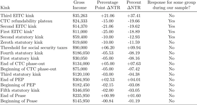
Table 2: Kinks faced by a single parent with two children in 2005, ranked by size Gross Income Percentage Point ΔNTR Percent ΔNTR
Response for some group during our sample? Kink
Third EITC kink $35,263 +21.06 +37.41 No CTC refundability plateau $24,333 -15.00 -19.66 Yes Second EITC kink $14,370 -21.06 -19.62 Yes First EITC kink* $11,000 -25.00 -18.89 Yes
Second statutory kink $59,400 -10.00 -12.93 Yes Zeroth statutory kink $19,600 -10.00 -11.59 No Threshold for social security taxes $90,000 +06.20 +09.94 No Fourth statutory kink $186,050 -05.53 -08.19 No First statutory kink $30,050 -05.00 -08.16 No End of CTC phase-out $134,000 +05.00 +07.63 No Beginning of CTC phase-out $75,000 -05.00 -07.42 No Third statutory kink $120,100 -03.00 -04.38 No End of PEP $304,950 +02.53 +04.01 No Beginning of PEP $182,450 -02.15 -03.08 No Fifth statutory kink $346,050 -02.00 -03.05 No End of Pease $235,950 +00.99 +01.60 No Beginning of Pease $145,950 -00.84 -01.19 No
Kinks are ranked in descending size, measured by percent change in the net-of-tax rate. See the caption of Figure 1 for our assumptions.
*The first EITC kink coincides with the CTC refundability kink.
6.1
Where Do Taxpayers Bunch?
Despite the predictions of standard economic theory, at most kinks there is no evidence of responsiveness in any of the years of our sample. This includes the largest kink in Figure 1, the non-convex kink at the end of the EITC phase-out region. As we discuss in Appendix E, standard theory predicts a dip in the distribution of income near a non-convex kink. We do not observe this in the data, even for groups that are highly sensitive to other kinks.
We also see no response at most statutory kinks, including the high-income kinks. This is somewhat surprising because the difference-in-difference literature (summarized in Section 3.1) has consistently found high-income filers to be more responsive to tax rates as they change over time.
In a separate attempt to find responses by high income tax units, we analyze the largest and highest income kinks created by state income tax regimes in California, Connecticut, and New Jersey. One disadvantage of state tax rates in a bunching context is that most generate small kinks (less than 3 percentage point changes), though the state tax regimes in these states contain some of the largest state kinks. The advantage of analyzing them is that many kinks affect taxpayers at income levels greatly exceeding any federal kink. However, we find no bunching at any of the state kinks we examined.
Our broad finding of zero responsiveness, even at large kinks, implies that taxable income is insensitive to marginal tax rates in the neighborhood of most kinks. This could be driven by several mutually compatible causes. First, it could be that taxpayers have imperfect knowledge of their local tax schedule. Second, taxpayers may not base their decisions on marginal incentives. Third, taxpayers may know their local schedule and want to respond to marginal incentives, but may be constrained by optimization frictions, such as adjustment costs or lumpy earnings opportunities. However, this third explanation is less convincing when deduction opportunities are present. Deductions, such as charitable giving, allow tax-payers to precisely manipulate their taxable income at the end of the tax year, after gross income is observed. Fourth, marginal tax rates are functions of annual income and deduc-tions. Individuals respond to marginal tax rates throughout the year based on expectations of income and deduction activity. If income is sufficiently volatile or expectations are suffi-ciently imprecise tax units might fail to respond to kink points. This problem is potentially compounded by the presence of multiple income earners and income types.
When kinks are small, the hypothesis that taxpayers ignore marginal incentives is partic-ularly appealing. Chetty (2012) shows that ignoring such kinks in the tax schedule generally leads to utility losses of less than 1% compared to utility-maximizing choice. In light of this, the lack of responsiveness at the PEP and Pease kinks as well as the fifth statutory kink is unsurprising.27
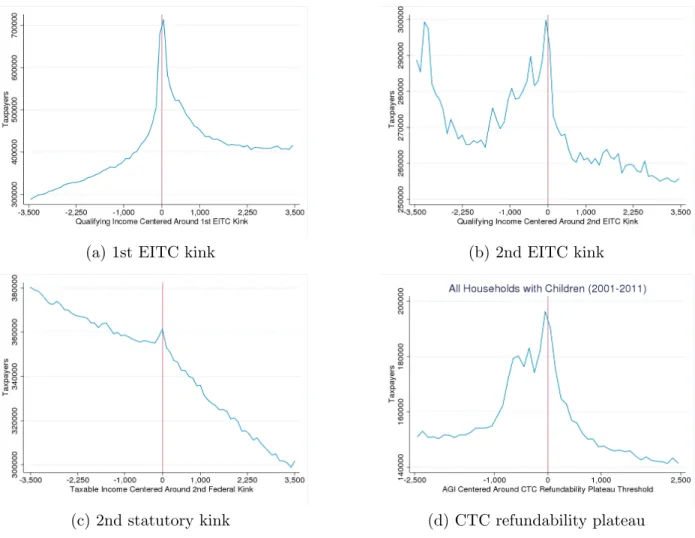
Taxpayers do not always behave at odds with standard economic theory, however. We find responsiveness to marginal incentives at several kinks. First, like Saez (2010) and Chetty et al. (2013), we find clear bunching patterns at the first EITC kink in all years of our sample. This is where the strongest bunching occurs. Second, we document new bunching phenomena at the second EITC kink, the second statutory kink, and the CTC refundability plateau kink. These responses can be seen in Figure 2, which groups together various household types for all years in which households are responsive. These patterns are explored in detail in the following sections.
6.2
Estimation Technique
When measuring bunching, the key issue is how taxpayers would behave in the absence of a kink. In particular, we must specify the alternative local tax schedule as well as the local distribution of income under the alternative tax schedule. We estimate this counterfactual behavior separately for two scenarios, corresponding to the two marginal tax rates (MTRs) that hold above and below the kink. Let us call 𝑡0 the MTR that applies below the kink,
and 𝑡1 the MTR that applies above it. First, for those bunchers located below (left of) 27In Appendix D we look for bunching at income eligibility thresholds for various transfer programs,
Figure 2: Bunching at four kinks
(a) 1st EITC kink (b) 2nd EITC kink
(c) 2nd statutory kink (d) CTC refundability plateau
Panels (a) and (b) feature all EITC-eligible filers in our sample, from 1996 to 2011 and 2002 to 2011, respectively, with the following exception. When the kinks are within $2,000, we drop all taxpayers in (a) that respond to the second kink, and we drop all taxpayers in (b) that respond to the first kink. Panel (c) includes all tax filers in our sample, 1996-2011. Panel (d) includes all tax filers in our sample with children, except those located within $2,000 of the first or second EITC kinks, 2004-2011.
the kink, we estimate their behavior under a locally constant MTR equal to 𝑡0. In other
words, we assume their MTR continues unchanged throughout the kink region. Second, for those bunchers located above (right of) the kink, we estimate their behavior under a locally constant MTR equal to 𝑡1, assuming their MTR also held below the kink.
In estimating these counterfactual scenarios separately, we break from the conventional bunching analysis developed by Chetty et al. (2011). To our knowledge, all extant research that reports bunching coefficients uses their style of estimating one counterfactual distribu-tion for bunchers on both sides of the kink. Though not always made explicit, the underlying assumption for the counterfactual tax schedule is a constant MTR equal to 𝑡0.
into elasticity estimates in Section 7. Researchers that use the Chetty et al. (2011) style of bunching estimation translate their coefficients into elasticities using an infinitesimal bunch-ing formula that is valid only for small kinks. In contrast, our estimation technique allows us to translate bunching coefficients into elasticities using Equation 3, which is appropriate for discrete jumps in MTRs.28 The differences in methods change the results quantitatively
but not qualitatively.29
For each counterfactual scenario, we estimate the income distribution using observed data near the kink but not so close as to be affected by bunching behavior. Specifically, we group households into bins and estimate distinct linear projections on both sides of the kink. For the counterfactual scenario where the MTR is𝑡0, we use bins−𝑅, ...,−1,0, where
bin 0 contains the kink. For the counterfactual scenario where the MTR is 𝑡1, we use bins
0,1, ..., 𝑅. We call the union of these sets of bins the “bunching region.”
For the counterfactual scenario where the MTR is𝑡0, we estimate the following equation
by ordinary least squares:
𝑦𝑗 =𝛼0+𝛽0𝑧𝑗+ 0
∑︁
𝑘=−𝑊
𝛾𝑘0·1[𝑗 =𝑘] +𝜀0𝑗, (4)
where 𝑦𝑗 denotes the number of taxpayers in bin 𝑗, 𝑧𝑗 denotes the income level of bin
𝑗, 𝑊 denotes the number of bins in the bunching window near the kink, and 𝜀0
𝑗 denotes
the residual.30 Parameters 𝛾0
𝑘 capture the number of taxpayers in the bunching window
unexplained by the linear prediction (𝛼0+𝛽0𝑧
𝑘). In other words, 𝛾𝑘0 measures the amount
of excess mass in bin 𝑘 relative to the counterfactual expectation.
For the counterfactual scenario where the MTR is 𝑡1, we estimate a similar equation:
𝑦𝑗 =𝛼1+𝛽1𝑧𝑗 + 𝑊
∑︁
𝑘=0
𝛾𝑘1·1[𝑗 =𝑘] +𝜀1𝑗. (5)
Our default parameter values, which we select by visual inspection, are 𝑅 = 35, 𝑊 = 10, and binwidth 𝛿 = $100. Our default counterfactuals are therefore derived from the actual distribution of income between $1,000 and $3,500 away from each kink. Letting circumflexes denote estimated coefficients, we calculate the total number of bunchers as
28See Section 2 for details. An additional concern with the approach of Chetty et al. is that it uses the
existing income distribution above the kink (i.e. under MTR 𝑡1) to inform the counterfactual distribution
under MTR 𝑡0. Saez (2010) shows these distributions are generally not equal, nor are they directly
pro-portional. Thus it is unclear what, if any, information the actual distribution above the kink offers when estimating the counterfactual distribution (under MTR𝑡0).
29We compare our methods with those of Chetty et al. (2011) and Saez (2010) in Section 7.3. In general,
our methods produce bunching coefficients smaller than Saez’s and larger than those of Chetty et al.
30We tried including higher-order polynomial terms of𝑧
𝑗, but this would often over-fit the data, producing
Figure 3: Actual and estimated counterfactual distributions of income
The distribution of income is displayed for married couples filing jointly in 2002 who have no capital gains realizations. The estimation parameters are𝑅= 18,𝑊= 5, and𝛿= $200.
^ 𝐵 = ∑︀−1 𝑘=−𝑊𝛾^ 0 𝑖 + ∑︀𝑊 𝑘=1^𝛾 1
𝑖 + (1/2)(^𝛾00 + ^𝛾01). Figure 3 shows this estimation technique in
action for married filers near the second statutory kink in 2002. The estimated number of bunchers is simply the difference between the observed and counterfactual distributions of income inside the bunching window.
When comparing bunching between groups, however, the total number of bunchers is a flawed metric. All else equal, the number of bunchers will be larger when analyzing more populous groups. Hence, we report a unitless bunching coefficient ^𝑏 equal to ^𝐵 divided by the average number of non-bunchers in $100 bins inside the bunching window. In other words, letting 𝑃𝑘 denote the observed population in bin 𝑘, we define
^𝑏≡𝐵/^ [︃ ∑︀𝑊 𝑘=−𝑊𝑃𝑘−𝐵^ 2𝑊 + 1 · 100 𝛿 ]︃ .
We use a bootstrap procedure to obtain standard errors for ^𝑏 by adding randomly sampled estimated residuals (from the original regressions) to the predicted values of the original regressions, repeatedly estimating ^𝑏 from the new, simulated data.31
6.3
Estimation Results
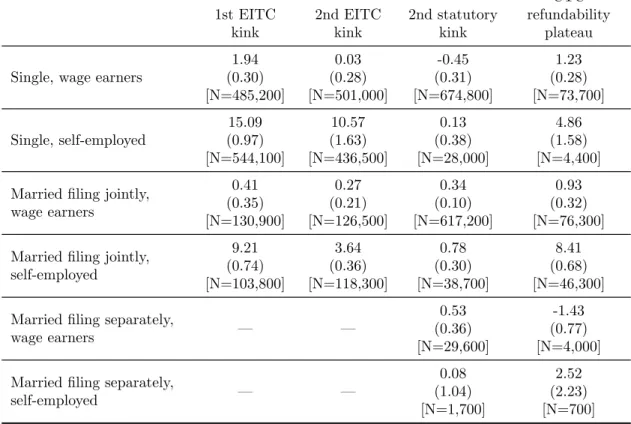
Though all taxpayers face incentives to bunch at the convex kinks of Figure 2, some taxpayers are more responsive to these incentives than others. To compare bunching patterns across groups, Table 3 presents estimated bunching coefficients at the four kinks where we find a response, using 2011 data. In general, the first EITC kink elicits the largest response. It sees the largest bunching coefficient, 15.09, corresponding to single, self-employed individuals. For this group, we calculate the mass of bunchers as approximately 15 times the average number of non-bunchers in $100 bins inside the bunching window. This implies 43% of taxpayers in the bunching window (i.e. within $1,000 of the kink) are there because of the changing marginal incentives at the kink.32 According to the theory developed in Section
2, these taxpayers desire income greater than the kink when facing the low tax rate, and income less than the kink when facing the high tax rate.
Other groups and other kinks exhibit smaller bunching coefficients, taking a range of values from -1.43 to 9.21.33 The range of the coefficients hints at the substantial heterogeneity
we observe across certain demographic characteristics and across kinks. Some aspects of this heterogeneity are systematic. For example, taxpayers with self-employment income are generally more responsive than pure wage earners (i.e. those without self-employment income). In Table 3, all of the statistically significant bunching coefficients for the self-employed are larger than those of their wage-earning counterparts. Most of these differences are themselves statistically significant. This finding is unsurprising given prior research that finds bunching only among the self-employed (Saez, 2010). Manipulating earned income is inherently easier when one is both the employer and employee, so the self-employed likely exhibit larger real labor responses. Moreover, unlike wage income, self-employment income is not subject to third-party reporting and is easier to hide from tax authorities (or inflate when income is subsidized). Thus, the self-employed likely exhibit larger tax evasion responses as well. It remains an open question which of these factors contributes more to the differential
31We thank Raj Chetty, John Friedman, Tore Olsen, and Luigi Pistaferri for public provision of a Stata
program designed specifically to implement their estimation technique. Our code builds directly on theirs, and we plan to make our code publicly available in the near future.
32To see this, let𝑋 denote the average number of non-bunchers in $100 bins inside the bunching window.
Then the fraction of bunchers among the population within $1,000 of the kink is 15.09𝑋/(2·10𝑋+15.09𝑋) = 15.09/35.09≈0.43.
33Negative numbers imply the kink causes less mass to locate near the kink. This is plausible only if
the ETI is negative, which has little empirical support. As none of the negative coefficients are statistically distinguishable from zero, we interpret them as evidence that taxpayers are not responding to the kink.
Table 3: Bunching coefficients calculated at four kinks in 2011 CTC refundability plateau 1st EITC kink 2nd EITC kink 2nd statutory kink Single, wage earners
1.94 0.03 -0.45 1.23 (0.30) (0.28) (0.31) (0.28) [N=485,200] [N=501,000] [N=674,800] [N=73,700] Single, self-employed 15.09 10.57 0.13 4.86 (0.97) (1.63) (0.38) (1.58) [N=544,100] [N=436,500] [N=28,000] [N=4,400] Married filing jointly,
wage earners
0.41 0.27 0.34 0.93
(0.35) (0.21) (0.10) (0.32) [N=130,900] [N=126,500] [N=617,200] [N=76,300] Married filing jointly,
self-employed
9.21 3.64 0.78 8.41
(0.74) (0.36) (0.30) (0.68) [N=103,800] [N=118,300] [N=38,700] [N=46,300] Married filing separately,
wage earners
0.53 -1.43
— — (0.36) (0.77)
[N=29,600] [N=4,000] Married filing separately,
self-employed
0.08 2.52
— — (1.04) (2.23)
[N=1,700] [N=700]
Bunching coefficients are reported for various household types, with standard errors in parentheses. The number of taxpayers in the bunching region (rounded to the nearest hundred) is presented in brackets. Wage earners are those with positive wage income and zero self-employment income. The self-employed are those with positive self-employment income. Single status includes “head of household” filers. Married filers who file separately are ineligible for the EITC and thus are excluded from its analysis.
in responsiveness between wage earners and the self-employed.34
Unlike prior research, however, the bunching responses we observe are not confined to the self-employed. Wage earners exhibit statistically significant bunching coefficients at each of the four kinks where we observe a response.35 Because wage earnings are reported
by third parties, they are known to be more reliable indicators of real economic activity (Slemrod, 2007). Further, because EITC kinks are determined by gross income, deductions are irrelevant. Thus, the wage-earner responses we see at the first and second EITC kinks are strongly suggestive of real labor supply responsiveness to marginal tax rates.
34In a tax audit experiment in Denmark, Kleven et al. (2011) find that around half of the bunching
response of the self-employed is eliminated post-audit, suggesting around half of the bunching response is due to tax evasion. This could underestimate the role of evasion, since audits only catch detectable evasion. However, it could overestimate the role of evasion if taxpayers make honest mistakes.
35Though Table 3 does not show it, the second EITC kink sees statistically significant coefficients for wage
6.3.1 Heterogeneity Across Demographics
We also see differentials in responsiveness across filing statuses and across household size. These patterns can be seen in Table 4, which gives bunching coefficients for the first two EITC kinks by filing status and number of children, using 2011 data. In general, single filers are more responsive than married filers. Among statistically significant coefficients, those of single filers are always larger than those of married filers. Several of these differences are themselves statistically significant, and all are relatively stable over time. This differential holds for both wage earners and the self-employed, suggesting that the real labor supply response of single filers is larger than that of their married counterparts. This may be because EITC-eligible single filers have a larger structural elasticity or because they are more knowledgeable about the EITC schedule.
Table 3 provides some evidence suggesting variation in knowledge about the credit may play a large role. There we see that single filers are not always more responsive around the CTC refundability plateau kink. In fact, the one statistically significant difference between single taxpayers and married taxpayers filing jointly indicates that married filers are more responsive. Because the CTC-eligible population overlaps heavily with the EITC-eligible population, we would expect a similar differential to exist across marital status in these two populations, provided all taxpayers were fully informed about both programs. The fact that the differential is reversed suggests that taxpayers are not fully informed. Instead, it appears single filers are better informed about the EITC and married filers are better informed about the CTC.
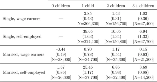
We also observe consistent differentials in responsiveness across tax unit size. At the first EITC kink, taxpayers with one child are the most responsive, with bunching coefficients up to 39.65. At the second EITC kink, however, taxpayers with two or more children are the most responsive, with bunching coefficients up to 11.64.36 The results at the second
EITC kink are less surprising than those at the first. Because the subsidy is more generous to taxpayers with more children, they face a greater change in effective tax rates at each kink. If taxpayers with similar incomes have the same structural elasticity and the same knowledge of the EITC schedule, regardless of number of children, then we should expect sharper bunching among taxpayers with more children. This is what we observe at the second kink.
At the first kink, however, the differential is reversed. Among parents, those with fewer
children exhibit the sharpest responses. On its face, this suggests that parents with one
36At the second statutory kink, we find no statistically significant differences in responsiveness by number
of children. Unfortunately, we cannot test this hypothesis at the CTC refundability kink, because for many numbers of children the kinks are too close to other kinks in the schedule to attribute the response to the CTC.
Table 4: Bunching coefficients calculated at two kinks in 2011 First EITC kink
0 children 1 child 2 children 3+ children Single, wage earners
2.85 1.43 1.02 — (0.43) (0.31) (0.36) [N=306,300] [N=156,700] [N=47,400] Single, self-employed 39.65 10.05 6.94 — (1.63) (1.34) (1.32) [N=224,100] [N=150,800] [N=47,700] Married, wage earners
-0.44 0.70 1.17 0.15 (0.49) (0.78) (0.54) (0.63) [N=38,000] [N=34,700] [N=35,300] [N=21,200] Married, self-employed 1.57 25.46 6.85 3.69 (0.86) (1.17) (0.98) (0.88) [N=26,600] [N=37,700] [N=32,400] [N=14,200]
Second EITC kink
0 children 1 child 2 children 3+ children Single, wage earners
-0.10 3.34 2.13 — (0.16) (0.24) (0.31) [N=322,600] [N=210,900] [N=76,000] Single, self-employed 2.56 9.72 11.64 — (0.90) (2.30) (2.06) [N=36,000] [N=99,200] [N=39,400] Married, wage earners
0.13 0.22 -0.20 1.08 (0.43) (0.43) (0.52) (0.50) [N=59,100] [N=58,800] [N=56,200] [N=36,700] Married, self-employed 3.16 0.69 1.65 7.33 (1.28) (0.45) (0.49) (0.56) [N=26,900] [N=17,700] [N=21,500] [N=21,800]
Bunching coefficients are reported for various household types, with standard errors in parentheses. The number of taxpayers in the bunching region (rounded to the nearest hundred) is presented in brackets. Estimates for single, childless taxpayers are omitted because their kinks are within $2,000, contaminating the estimation procedure. Married taxpayers are excluded if filing separately. Wage earners are those with positive wage income and zero self-employment income. The self-employed are those with positive self-employment income. Single status includes “head of household” filers.
child either have a larger structural elasticity or are better informed about the first EITC kink. The results at the second EITC kink, however, work against the structural-elasticity explanation. Once again, the fact that a differential is reversed for two similar populations at two different kinks implies that variation in knowledge plays a large role in mediating responses to tax incentives. It seems taxpayers with one child are better informed about the first EITC kink – enough to overwhelm the smaller bunching incentives. In contrast,
taxpayers with two or more children appear relatively more informed about the second EITC kink.
6.3.2 Additional Sources of Heterogeneity
In this section, we compare bunching patterns across a number of other observable charac-teristics, including age, sex, number of earners, industry of occupation, and whether or not tax forms were filed electronically. We focus exclusively on the first EITC kink, where we see the largest responses. Table 5 displays selected bunching coefficients using 2011 data.
Sex The conventional difference-in-difference literature finds that females are more sensitive to marginal tax rates than males (McClelland and Mok, 2012). In particular, studies focusing on the labor-supply effects of the EITC have shown females to be more responsive than males (Nichols and Rothstein, 2015). Our bunching evidence mostly supports this finding. Among the self-employed, we find that females exhibit stronger bunching patterns than males in every year of our sample. Their bunching coefficients tend to be about twice that of males, though the gap narrows in the last few years of our sample. Among wage earners, females have larger bunching coefficients every year from 1996 to 2008, but this differential is statistically insignificant, and reverses in the last three years of our sample.
Secondary Earners The conventional literature generally finds that secondary earners have more flexible labor supply than primary earners (McClelland et al., 2014). Thus we expect married couples with two wage earners to be more sensitive to changing tax rates at kinks than married couples with one wage earner. However, when we focus exclusively on wage earners, married couples’ responses are almost always statistically insignificant. Thus we compare households with both wage earnings and self-employment income, comparing those with one wage earner and those with two. Unfortunately, we do not observe whether one or two spouses earn self-employment income. The results are inconclusive. The 2011 coeffi-cients displayed in Table 5 show that households with a single earner bunch more. But for most other years the differential is statistically insignificant, and for some the differential is reversed: dual earners are more responsive. Though our results point towards similar responsiveness between one- and two-earner households, we do not put much confidence in this finding because self-employment income seems to be the operative channel for response. In general, households with both wage earnings and self-employment income do not yield statistically different results than households with self-employment income alone. Our com-parison between households with one or two wage earners is therefore likely uninformative about the effects of a secondary earner on bunching patterns.
Table 5: Bunching coefficients calculated at the first EITC kink in 2011 Single Married filing jointly Wage earners Self-employed Wage earners Self-employed Males 2.39 11.49 (0.41) (0.71) — — [N=111,800] [N=187,200] Females 1.80 17.07 (0.30) (1.06) — — [N=373,300] [N=356,800] One wage earner
0.27 10.55
— — (0.46) (0.52)
[N=99,100] [N=32,300] Two wage earners
0.87 7.30 — — (0.42) (0.74) [N=31,800] [N=7,000] Ages 18-30 1.41 17.89 0.28 10.40 (0.25) (1.21) (0.39) (0.80) [N=221,900] [N=176,900] [N=32,800] [N=13,900] Ages 31-50 2.20 15.28 0.93 9.24 (0.34) (0.98) (0.47) (0.91) [N=211,400] [N=273,300] [N=55,100] [N=51,100] Ages 51+ 3.31 9.58 -0.10 8.75 (0.61) (0.62) (0.51) (0.76) [N=50,900] [N=92,900] [N=42,900] [N=38,700] Electronic filers 1.87 16.63 0.29 10.10 (0.28) (0.96) (0.35) (0.81) [N=459,900] [N=465,900] [N=115,100] [N=83,200] Paper filers 3.23 6.81 1.31 5.75 (0.54) (0.56) (0.72) (0.86) [N=25,200] [N=78,300] [N=15,800] [N=20,500] Bar or restaurant employees
0.92 18.91 -0.50 9.44 (0.26) (0.97) (0.71) (1.66) [N=55,900] [N=22,600] [N=7,900] [N=1,800] Full sample 1.94 15.09 0.41 9.21 (0.30) (0.97) (0.35) (0.74) [N=485,200] [N=544,100] [N=130,900] [N=103,800]
Bunching coefficients are reported for various household types, with standard errors in parentheses. The number of taxpayers in the bunching region (rounded to the nearest hundred) is presented in brackets. Wage earners are those with positive wage income and zero self-employment income. The self-employed are those with positive self-employment income. Single status includes “head of household” filers. Taxpayers under 25 or over 65 years of age who do not have children are ineligible for the EITC and are therefore excluded. Paper filers are defined as those who do not file electronically.
earners and the self-employed. Among single, self-employed taxpayers, the youngest age group (ages 18-30) has the largest bunching coefficients and the oldest age group (ages 51+) has the smallest bunching coefficients every year in our sample. For most years, these differentials are statistically significant. For their married counterparts, the same pattern holds from 1996 to 2007. However, from 2008 to 2011 the coefficients look very similar across age groups, and are never statistically distinguishable. Overall, the evidence points towards younger self-employed taxpayers being more responsive, with the gap closing over time. Among wage earners, most bunching coefficients are statistical zeros. However, single wage earners have significant bunching coefficients starting in 2009. For this group, it is the older taxpayers who show stronger bunching patterns.
Electronic filing Next we compare taxpayers who file electronically and those who file using paper forms. It is not clear what to expect. On the one hand, electronic filers are likely to be technologically savvier and are potentially more likely to be filing through a paid preparer.37 On the other hand, paper filers are confronted with the credit’s schedule when they fill in their tax forms, so they might be better informed about kink locations.38 We find that, among the self-employed, taxpayers filing electronically consistently exhibit bunching coefficients two to four times as large as those of paper filers. Among wage earners, the two groups are statistically indistinguishable throughout most of our sample. In later years, though, wage-earning paper filers have larger bunching coefficients than electronic filers. These wage-earner differentials are statistically significant for single filers in 2010 and 2011.
Industry Being employed in certain industries may make bunching easier to achieve. In Denmark there is evidence that workers in highly unionized industries, such as the teaching profession, show stronger bunching patterns (Chetty et al., 2011). Kink points may provide anchors for wage negotiations there. In addition, industries with widespread tipping practices may make tax evasion easier for employees. To test these hypotheses, we compare bunching patterns across all twenty two-digit NAICS codes.39 Virtually all industries, including heav-ily unionized industries, show no difference in bunching patterns. The one industry with a convincingly different response pattern was that of accommodation and food services. We further isolated the group responsible using three-digit NAICS codes. We report the bunch-ing coefficients of bar and restaurant workers in Table 5. When we focus on wage earners, the data do not support the hypothesis that workers in this tip-heavy industry have stronger
37The data do not allow us to distinguish between those using a paid preparer and those filing
indepen-dently.
38This assumes electronic filers are more likely to use tax preparation software, which typically keep tax
schedules hidden from view.
bunching patterns compared to the full population. Most years see statistically insignificant bunching coefficients, and if anything wage-earning bar and restaurant workers bunch less
in later years of the sample. However, among employees who also earn self-employment income, bar and restaurant workers exhibit larger bunching coefficients in every year of our sample. For married taxpayers, the differentials are not typically statistically significant, but for single taxpayers they almost always are.
Taken as a whole, our findings show that responsiveness to marginal tax rates is subject to substantial variation throughout the population. Taxpayers respond differently based on their age, sex, number of children, method of filing, industry of employment, and, most importantly, their self-employment status. This heterogeneity is problematic for the con-ventional regression approach to estimating sensitivity to tax rates, which relies on the assumption that tax sensitivity is constant across diverse subpopulations. Another poten-tially problematic issue in the conventional literature is that tax sensitivity is assumed to be constant over time. In the Section 7.2, we provide evidence suggesting this assumption, too, is unlikely to hold.
6.4
Bunching Puzzles
There are a few bunching patterns we observe that we are unable to explain, as taxpayers appear to react to non-existent incentives. Some of these bunching patterns are quite sharp, implying a strong behavioral response. However, we do not know what perceived incentives taxpayers are responding to. Each bunching pattern we identify in this section does not align with EI