Statistical Methods for Analyzing Complex Spatial and Missing Data

(1)

Statistical Methods for Analyzing

Complex Spatial and Missing Data

The Harvard community has made this

article openly available. Please share how

this access benefits you. Your story matters

Citation Antonelli, Joseph. 2016. Statistical Methods for Analyzing Complex Spatial and Missing Data. Doctoral dissertation, Harvard University, Graduate School of Arts & Sciences.

Citable link http://nrs.harvard.edu/urn-3:HUL.InstRepos:26718722

Terms of Use This article was downloaded from Harvard University’s DASH repository, and is made available under the terms and conditions applicable to Other Posted Material, as set forth at http://

nrs.harvard.edu/urn-3:HUL.InstRepos:dash.current.terms-of-use#LAA

(2)

Statistical methods for analyzing complex spatial

and missing data

A dissertation presented

by

Joseph Lawrence Antonelli

to

The Department of Biostatistics

in partial fulfillment of the requirements

for the degree of

Doctor of Philosophy

in the subject of

Biostatistics

Harvard University

Cambridge, Massachusetts

September 2015

(3)

c

(4)

Dissertation Advisors: Brent Coull and Francesca Dominici Joseph Lawrence Antonelli

Statistical methods for analyzing complex spatial

and missing data

Abstract

In chapter 1, we develop a novel two-dimensional wavelet decomposition to decom-pose spatial surfaces into different frequencies without imposing any restrictions on the form of the spatial surface. We illustrate the effectiveness of the proposed decomposi-tion on satellite based PM2.5 data, which is available on a 1km by 1km grid across

Mas-sachusetts. We then apply our proposed decomposition to study how different frequen-cies of the PM2.5 surface adversely impact birth weights in Massachusetts.

In chapter 2, we study the impact of monitor locations on two stage health effect studies in air pollution epidemiology. Typically in these studies, estimates of air pollution exposure are obtained from a first stage model that utilizes monitoring data, and then a second stage outcome model is fit using this estimated exposure. The location of the monitoring sites is usually not random and their locations can drastically impact inference in health effect studies. We take an in-depth look at the specific case where the location of monitors depends on the locations of the subjects in the second stage model and show that inference can be greatly improved in this setting relative to completely random allocation of monitors.

In chapter 3, we introduce a Bayesian data augmentation method to control for founding in large administrative databases when additional data is available on con-founders in a validation study. Large administrative databases are becoming increasingly available, and they have the power to address many questions that we otherwise couldn’t answer. Most of these databases, while large in size, do not have sufficient information on confounders to validly estimate causal effects. However, in many cases a smaller, val-idation data set is available with a richer set of confounders. We propose a method that

(5)

uses information from the validation data to impute missing confounders in the main data and select only those confounders which are necessary for confounding adjustment. We illustrate the effectiveness of our method in a simulation study, and analyze the effect of surgical resection on 30 day survival in brain tumor patients from Medicare.

(6)

Acknowledgments

I would like to thank my advisors, Brent Coull and Francesca Dominici, for an incred-ible experience working with you both. I can’t imagine a better and more supportive set of advisors who I consider to not only be great mentors, but more importantly also great friends.

I would also like to thank Cory Zigler and Joel Schwartz for their invaluable advice throughout my time working on these projects. Whether it was at committee meetings or random times that I stopped by your offices I knew that I could come to you guys for help on projects and I would come away with new ideas and a new perspective.

I would also like to thank all my friends that I’ve made in my time here in Boston, especially those from the Biostatistics department. There are too many people to name here, but they’ve made my time in Boston special and it’s because of them that I now consider Boston home, something I never thought I would say when I arrived here.

I would especially like to thank Georgia Papadogeorgou for being an amazing person and partner. You’ve been incredibly supportive of me and you always push me to bigger and better things. The last two years have been special in many ways and that is all a credit to how much you mean to me.

Finally, I would like to thank my parents and my brother who have all shaped me into the person that I am today. None of this would be possible without you guys, and I consider myself very lucky to call you my family.

(10)

Spatial multiresolution analysis of irregularly spaced grids

with application to the effect of PM

2.5

on birth weights

Joseph Lawrence Antonelli

Department of Biostatistics

Harvard Graduate School of Arts and Sciences

Joel Schwartz

Department of Biostatistics

Harvard Chan School of Public Health

Itai Kloog

The Department of Geography and Environmental Development

Ben-Gurion University of the Negev

Brent Coull

Department of Biostatistics

(11)

1.1 Introduction

The epidemiologic literature investigating the health effects of air pollution has become vast, as countless studies have found associations between ambient levels of air pollu-tion and a variety of adverse health outcomes (Dockery et al. (1993); Samet et al. (2000); Dominici et al. (2006) and a review of the literature is provided by Dominici et al. (2003); Pope III (2007); Breysse et al. (2013)). Despite the large number of studies investigating the relationship between air pollution exposures and human health, there still exist criti-cal and unanswered questions that need to be addressed for the establishment of new reg-ulations. Currently the EPA regulates total PM2.5 levels, however, PM2.5 is comprised of

many different components and sources of pollution . An important question is the extent to which various sources of pollution adversely affect health, knowledge of which could lead to more effective targeted regulations. Establishing the extent to which fine scale, local pollution or long range regional transport pollution is associated with health effects would be very useful in planning future air regulations on lowering air pollution stan-dards. Furthermore, isolating different sources of air pollution would allow researchers to gain valuable information regarding the chemical composition of PM2.5 in different

regions, and potentially quantify the health impacts of these separate components. There have been very few attempts to jointly model the health effects of long range pol-lution and local polpol-lution sources such as traffic, though it remains a crucial question in air pollution epidemiology. Maynard et al. (2007) used a variety of atmospheric, weather, and land use variables to predict black carbon levels for individuals in the Boston area. Black carbon (BC) is known to be highly associated with local traffic pollution. Sulfates are known to be spatially homogenous and represent long range pollution sources such as coal fired power plants, and the investigators examined the joint health effects of these two exposures. Other articles have decomposed air pollution into local and regional sources without subsequently examining their respective effects on health. Moreno et al. (2009) examined the differences in hourly fluctuations of traffic and urban background components of PM10 in Santander, Spain. Brochu et al. (2011) used quantile regression to estimate the regional and local components of BC in Boston and investigated how the

(12)

sources of BC changed both across the year and within a given day.

Due to recent advancements in PM2.5 exposure estimation, we no longer need to rely

solely on PM2.5 monitors, as remote sensing satellite data can now yield reliable PM2.5

estimates on a 1km by 1km grid (Kloog et al., 2014). These new estimates of PM2.5 are on

a scale fine enough to allow novel approaches to spatial decomposition based on image analysis techniques. We show such decompositions of PM2.5 can yield insights into the

sources of pollution most associated with health effect estimates. A variety of methods have been proposed to decompose surfaces into different spatial scales, two of the most common such techniques are wavelet decompositions and Fourier decompositions. For the remainder of the manuscript we focus discussion on wavelets. Due to the existence of point and line sources of pollution, such as interstates and other roadways, the surface of PM2.5 will contain many spikes. Wavelets are well known to be a useful basis

func-tion for preserving sharp features of data (Petrosian and Meyer, 2013), and many spike detection algorithms are based on wavelet transforms (Hulata et al., 2002; Nenadic and Burdick, 2005). One of the main goals of the study is to characterize the impact of traffic pollution sources on health and therefore it is important to adequately capture, and not over smooth, these spikes in the data. Moreover, wavelets decompose a spatial surface into multiple spatial scales that are orthogonal, which allows us to avoid multicolinearity and the resulting instability of effect estimates in a health effects model.

Standard two-dimensional Wavelet decompositions typically require that the surface be-ing decomposed is rectangular and the points are uniformly spaced. An additional re-quirement of standard wavelet analysis is that the points are dyadic, meaning that the number of points on the surface grid is 2l where l is some positive integer, although ”padding” the practice of adding points to the surface can be used to satisfy this require-ment. Our interest focuses on decomposing a spatial surface of PM2.5, a setting in which

none of these conditions are met. The coastline of the U.S is far from rectangular. There is no reason to think our data would be dyadic, and the satellite data yielding the PM2.5

estimates is not on a perfectly uniform grid. Previous work has avoided the dyadic as-sumption as well as the uniform grid asas-sumption through a variety of techniques such as the lifting scheme and interpolation (Sweldens, 1998; Xiong et al., 2006; Pollock and

(13)

Cas-cio, 2007; Gupta et al., 2010). Others have generalized Wavelet theory using radial basis functions, which are not constrained to lie on a uniform grid (Buhmann, 1995; Chui et al., 1996). To the best of our knowledge, however, none of these have provided a practical way of decomposing a surface that is not rectangular. In this paper we develop a two-dimensional extension to work originally proposed in Wand et al. (2011), which relaxes these assumptions of a standard wavelet analysis. The advantages of this method include its simple application, its ability to scale to large spatial surfaces, and its ability to avoid restrictive assumptions about the nature of our surface.

In this paper we will use the proposed wavelet based method to decompose daily sur-faces of PM2.5 across New England and use the components of the resulting decomposed

surface as covariates in a health effects model relating birth weight in Massachusetts to scale-specific PM2.5. Section 1.2 introduces the pollution data and motivating scientific

problem. Section 1.3 introduces the proposed method for performing 2d wavelet decom-positions on irregular grids. Section 1.4 illustrates the decomposition in the PM2.5 data.

Section 1.5 applies the method to analyze the association between scale-specific PM2.5and

birthweights in Massachusetts, and Section 1.6 concludes with further discussion.

1.2 PM

2.5

and Birthweights in Massachusetts

1.2.1 Exposure data

Typically PM2.5is measured at monitoring stations, which are located sporadically across

the United States. In early health effect studies, conditional on the monitoring values exposure to PM2.5 was assigned to be the value from the nearest monitor or a weighted

average of monitors within a pre-defined range. In recent years monitoring data has been augmented with geographical and remote sensing information to yield individual, resi-dence specific estimates of PM2.5levels. Specifically, in previous work we have combined

ideas from land use regression and mixed models, and incorporated satellite aerosol op-tical depth (AOD) measurements to obtain widespread estimates of PM2.5 at a 1 x 1 km

resolution (Kloog et al., 2014). Satellite AOD is a measure of light attenuation in the atmo-spheric column that is affected by ambient conditions and can be used to help estimate

(14)

PM2.5. Satellite estimates of PM2.5 on a 1km grid are available daily from 2003 to 2011

for the Northeastern United States and they give an accurate estimate of the surface of PM2.5in this area. Kloog et al. (2014) showed theR2values between predictions and true

values observed at monitors is around 0.9 indicating high predictive accuracy, although this only applies to areas with monitors and therefore doesn’t give much insight into the performance of the predictions in rural areas. Despite potential drawbacks of the surfaces being estimated, the fine scale nature of the exposure surface allows us to apply our pro-posed decomposition method and examine the effects of air pollution at a wide range of spatial scales.

1.2.2 Birth weights

Many epidemiological studies have established relationships between PM2.5and adverse

birth outcomes. Glinianaia et al. (2004); Dadvand et al. (2013) provide a review of the lit-erature. In Massachusetts, Kloog et al. (2012) reported an association between PM2.5 and

birth weights using Satellite AOD based PM2.5estimates on a 10km by 10km grid. We

ex-tend this work by using the finer scale, 1km satellite based PM2.5estimates as well as

esti-mating associations between birthweight and specific spatial-scales of variation of PM2.5

exposure. Kloog et al. (2012) provided specific details of the birthweight data. Briefly, the study population includes all singleton live births from the Massachusetts Birth Reg-istry from January 1st, 2000 to December 31st, 2008. We restrict attention to births after October 1st, 2003 as the satellite based PM2.5 data is only available from 2003 onwards.

The data set contains 332,717 singleton births and the geocoded address of each mother at the time of birth. This data combined with the satellite data described above and our proposed Wavelet decomposition as described in section 1.3 should provide insight into the different health impacts of local and regional sources of PM2.5.

(15)

1.3 Wavelet decomposition for irregular grids

1.3.1 Standard wavelet analysis

To motivate our approach and establish notation, we begin with a standard one-dimensional Wavelet decomposition. We will then extend the standard Wavelet decom-positions to that seen in Wand et al. (2011) which removes the issue of the data lying on a uniform grid. Finally, we will extend this approach to the two dimensional setting as our approach is a two-dimensional extension from that seen in Wand et al. (2011). For now, imagine that we have data, y, which is a function of x, dyadic, and equally spaced on the interval [0,1). In this case we haveR = 2L_{equally spaced data points, which leads to K}

=R−1basis functions. We are trying to represent our data in the following form as the sum of Wavelet basis functions

y=f(x) =θ0+ K X k=1 θkzuk(x), (1.1)

where y is our data, andzk are wavelet basis functions. Wavelet coefficients have a nice

interpretation in terms of scale and location of the function they are trying to represent. At level l there are2l−1basis functions, which move from left to right in terms of the support of each function. The lower level basis functions represent low frequency changes in our function, while the higher level basis functions represent the higher frequency changes in the function. Going back to our motivating example of PM2.5 this means that the

lower level functions will capture smooth, regionally varying trends in pollution, while the higher level functions will capture local PM2.5 changes such as interstates. Therefore

our basis functions are zu

1()which is the 1 function and represents level 1,z2u()and z3u()

which represent level 2, and so on for levels 3 to L. The above formulation can be rewritten as

(16)

where row i of the W matrix takes the following form 1z₁u(i−1 R )... z u R−1( i−1 R ) . (1.3)

In this case, determination ofθis trivial since the orthogonality of W leads to

θ =WTy. (1.4)

A variety of standard wavelet basis functions can be used and for this paper we will stick to the family of Debauchies wavelets, however, this choice is not of crucial importance for illustrating the method.

1.3.2 One dimensional penalized wavelets

Now that we have introduced some preliminary notation and the standard setup for this problem we can move to the case where the data is not on a regular grid. What this means is that we now have data,yif ori = 1...nobserved at locationsxif ori = 1..nwhere we have

imposed no restrictions about the location and dimension of y. We can define a new set of basis coefficients as

zk(x) = zku(

x−a

b−a), k = 1...K, (1.5)

where a and b are the minimum and maximum of x respectively, so we are essentially normalizing our data to lie in the interval [0,1). Now the problem lies in estimatingz_ku()at arbitrary points within the unit interval, since standard Wavelet basis functions using the discrete wavelet transform can only be evaluated via a recursive algorithm on a dyadic grid. The trick to doing this proposed by Wand et al. (2011) is to define a very fine grid of points on the unit interval, with the number of points in our grid being a multiple of 2. We are able to evaluate the basis functions on this grid and we will pick this grid to include a large number of points such as R=16,384 so that any of our data points will lie

(17)

very closely between two grid points. We could then calculate the value of zu

k() at any

point in the interval as a linear interpolation of the two nearest grid points as

z_ku(x)≈ {1−(xR− bxRc)}z_ku bxRc R + (xR− bxRc)z_ku bxRc+ 1 R , (1.6) and using this we can define a matrix Z as

Z =      1 z1(x1) . . . zK(x1) 1 z1(x2) . . . zK(x2) .. . ... ... 1 z1(xn) . . . zK(xn)      (1.7)

Now that we have defined wavelet basis functions and how to evaluate them at arbitrary locations, we simply need to estimate the coefficients corresponding to our basis func-tions. This can be done very easily in any standard regression framework, since we are in the following linear model situation

y=Zθ+, (1.8)

where is a mean zero vector of noise. The term ’penalized wavelets’ refers to the sit-uation where we find the wavelet basis coefficients using a penalized regression frame-work such as LASSO or ridge regression. For now we will estimate the parameters using LASSO as this turns out to be a better penalty for our pollution example in section 5. Our estimate ofθis defined by ˆ θ=arg min ( _n X i=1 (yi −Ziθ) 2 ) subject to X j |θj|< c, (1.9)

where c is a tuning parameter that controls the amount of penalization (Tibshirani, 1996). Now we’ve shown how to represent a function with wavelet basis functions on any grid and any number of data points. Using this we can decompose a function to investigate how a function changes at different frequencies, by only looking at the elements of θ

(18)

that correspond to the scale we are interested in. Our motivating example, however, is the surface of air pollution in New England and therefore requires a two dimensional wavelet decomposition, which we detail in the following sections.

1.3.3 Standard two dimensional wavelets

Again let us assume we are in the standard framework for wavelets where we have dyadic data on a uniform grid, however, now our data lies on a two dimensional sur-face. Our data, y, now takes the form of a 2L by 2L matrix and we wish to decompose it into different frequencies. Performing a two dimensional wavelet decomposition of this data is analogous to performing a one dimensional wavelet transform on the rows of y and then performing another one dimensional wavelet transform on the columns of the resulting matrix. Intuitively in a two dimensional plane this is like doing a wavelet transform in one direction (x1) and then doing it in the second direction (x2). This can be

written out as

y=Wx1_θT_Wx2T_, _(1.10)

where in this setting, Wx1 ₌ _Wx2 _{and both are defined in the same manner as our W}

matrix from the one dimensional section. We keep the two matrices separated byx1 and

x2 at the moment for generalizability and to maintain notation in the following section

when we introduce two dimensional wavelets for non dyadic and irregular data patterns. One thing to note is any row a and column b of y can be written as

yab = 2L X i=1 2L X j=1 Wx1 aiθijWbjx2, (1.11)

and this is important because it shows that the data is linear inθ and quadratic in the W matrices, suggesting that we could potentially fit this in a linear model framework just as in the one dimensional case. What we mean by that is if we write y as a vector instead of a matrix, we can write any element a of the vector y as

(19)

ya= 2L X i=1 2L X j=1 θijAij, (1.12)

whereAij is the corresponding quadratic function of elements of the W matrices. This is

important because we can now write the data in the usual regression framework

y=W∗θ, (1.13)

where W∗ is a design matrix with the appropriate elements, Aij, and then we can solve

for the wavelet coefficients using regression techniques. We will now show in the fol-lowing section how we can extend our ideas from the one dimensional setting to the two dimensional setting to perform a Wavelet decomposition for irregular data by the same logic.

1.3.4 Two dimensional penalized wavelets

In the one dimensional setting when we were on an irregular grid we came up with a new basis function by defining

zk(x) = zku(

x−a

b−a), k = 1...K, (1.14)

and then linearly interpolating on a fine grid to calculate the value of this function for any arbitrary point. Imagine now that we again have n data points, y_i∗, i = 1...n, which lie on a two dimensional space with the locations defined byx1i andx2i. In the motivating

example, y would be PM2.5 levels andx1 andx2 would be longitude and latitude

respec-tively. We can perform the one dimensional wavelet transform on an irregular grid in both thex1andx2 directions. We can define analogous functions for both directions as

zx1 k (x1) = zku( x1−a1 b1−a1 ), k= 1...K (1.15) zx2 k (x2) = z u k( x2 −a2 b2−a2 ), k= 1...K, (1.16)

(20)

where a1 and b1 define the range of x1, and a2 and b2 the range of x2. Using these we

can define matrices that are analogous to the Z matrix we defined in the one dimensional setting Zx1 ₌      1 zx1 1 (x11) . . . z_Kx1(x11) 1 zx1 1 (x12) . . . zKx1(x12) .. . ... ... 1 zx1 1 (x1n) . . . zKx1(x1n)      Zx2 ₌      1 zx2 1 (x21) . . . z_Kx2(x21) 1 zx2 1 (x22) . . . zKx2(x22) .. . ... ... 1 zx2 1 (x2n) . . . zKx2(x2n)      (1.17)

and now that we have defined these matrices as such, we can plug them into 1.12 to obtain the following representation of our data

y_a∗ = K X i=1 K X j=1 Zx1 aiθijZajx2 a= 1...n. (1.18)

If we think about how we solved for the wavelet coefficients in the one dimensional set-ting using penalized regression we can start to see how we can solve for the estimated coefficients in this case as well. If we define a design matrix as

Z∗ =      Zx1 11Z x2 11 Z x1 11Z x2 12 . . . Z x1 1KZ x2 1K Zx1 21Z x2 21 Z x1 21Z x2 22 . . . Z x1 2KZ x2 2K .. . ... ... Zx1 n1Z x2 n1 Z x1 n1Z x2 n2 . . . Z x1 nKZ x2 nK      (1.19)

then we are now essentially in the standard regression setup of

y∗ =Z∗θ+, (1.20)

and as before we can solve forθˆusing

ˆ θ=arg min ( _n X i=1 (y_i∗−Z_i∗θ)2 ) subject to X j |θj|< c. (1.21)

Note that because of the way we defined our wavelet basis functions we have not im-posed any restrictions on the dimension or shape of the two dimensional surface we are

(21)

representing. Once the Z∗ matrix is defined the method is trivial to implement and we can examine particular values of θ to determine how the surface changes at certain fre-quencies or scales.

1.4 Application to satellite PM

2.5

data

Now we will apply our method for two dimensional wavelet decompositions on each day of PM2.5 data in New England. We will restrict attention to a subset of New

Eng-land that surrounds Massachusetts as this will be the area of interest in the analysis of birth weights. The goal of the method is to separate different sources of pollution, which vary at different spatial frequencies. Previous work in air pollution exposure assessment has established that pollution separates into three different sources that vary at different spatial distances: Large scale regional pollution, pollution sources contributing to urban background, and sources of localized pollution such as traffic. Within the study region, re-gional sources of pollution will not vary spatially very much within a given day, though can vary greatly from day to day. This suggests that regional pollution sources will be represented by temporal variation in PM2.5, while the urban and local traffic sources will

be represented by spatial variability. Urban pollution sources should be represented by lower level Wavelet coefficients as they vary over longer distances. These are represented by differences in pollution between cities and rural areas. Local pollution sources, repre-sented by the higher level Wavelet coefficients, are those that vary quickly across space as they are caused by things such as interstates, and quickly fade away across space.

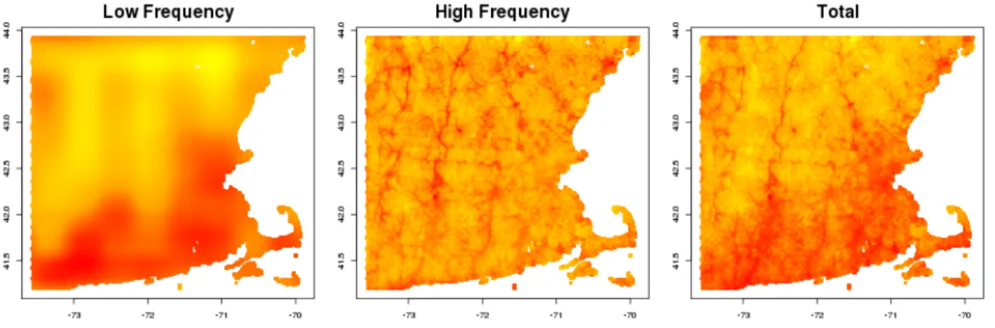
Figure 1.1 illustrates the average of our Wavelet decompositions across each day in 2006 for New England. We are able to see how the pollution surface breaks into two separate components, representing different spatial frequencies at which pollution changes. To create the lower frequency component seen in figure 1.1 we create a new vector of co-efficientsθ˜which is equal to θˆwith the exception that the coefficients corresponding to higher frequency basis functions are set to zero. We can then obtain a predicted lower frequency component via Z∗θ˜. To obtain a high frequency component as seen in figure 1.1 we could apply the same process, where instead we set the coefficients

(22)

correspond-Figure 1.1: Illustration of average wavelet decomposition averaged over the satellite data for 2006. The left panel shows the true surface, the middle panel is the high frequency component from our Wavelet decomposition, and the right panel is the low frequency component from our Wavelet decomposition.

ing to low frequency basis functions to zero. Alternatively, we could just take difference between the true surface and the lower frequency component as the higher frequency component.

One issue with separating the pollution surface into two different components, is the se-lection of a cutoff for what is deemed to be low frequency. In figure 1.1 we considered ba-sis functions to be low frequency if they represented levels 1 through 3 in either direction (latitude or longitude). Alternatively we could have considered basis functions that rep-resented levels 1 through 2 in each direction as representing low frequency changes, and this would have led to a slightly smoother surface for both the low and high frequency surfaces. For the analysis of birth weights we will use basis function levels 1 through 3 to represent low frequency changes in pollution. We decided upon this threshold both by vi-sual inspection as the decomposed surfaces appear to represent changes of interest to the air pollution epidemiology literature, and by examining the physical distances associated with each wavelet basis functions support. Note that while this decision is subjective, it is not of great importance as we will examine the effect of all spatial scales simultaneously regardless of their status as ”low” or ”high” frequency.

(23)

1.5 Analysis of birth weight data

We applied our proposed decomposition to examine the impact of PM2.5at different

spa-tial scales on birth weights in Massachusetts for the period 2003-2008. We perform the Wavelet decomposition for each day in the study period to obtain pollution surfaces rep-resenting different spatial scales.

1.5.1 Low vs High frequency components

First we examine the extent to which low and high frequency sources of pollution impact birth weight. We define the low frequency PM2.5component to be represented by scales 1

through 3, and the high frequency component to be scales 4 through 7. When looking at birth weights as an outcome our exposure can be defined either in terms of the mother’s full gestation period, a given trimester, or the last 30 days of the gestation period, though for the purposes of this paper we will restrict attention to the individual trimesters. This leads to a temporal component in the exposure as well as a spatial component, because we are looking at exposures averaged across time. Due to this we split our exposure surface for each day into three separate components: A mean component that is simply the mean PM2.5 for Massachusetts on the day of interest, a low frequency spatial component, and

a high frequency spatial component. For a particular mother in the study, these three exposure components computed for each day are then averaged across the trimester of interest. The idea in separating out the mean component from the surface is that it will capture temporal variation in PM2.5 levels and allow the low and high frequency scales

to solely represent spatial variability.

We will examine the effects of PM2.5at different scales using one of two models. The first

model is defined as follows:

BWij = (β0+β0j) +β1PM2.5ij +βcCij+ij, (1.22)

where the subscript ij represents subject i in census tract j. PM2.5ij is the overall PM2.5

(24)

to control for any correlation among mothers in similar neighborhoods. The vector Cij

represents all potential confounders we have included. ij is a mean zero, normal error

component. Details of the model choice and confounder selection can be found in Kloog et al. (2012). This model does not use any of the spatially decomposed PM2.5 exposures,

and thereforeβ1represents the combined effect of all PM2.5spatial scales.

To examine how different spatial scales of PM2.5 affect birth weight we will also examine

the following model:

BWij = (β0∗+β

∗

0j) +β

∗

1Meanij +β2∗Lowij +β3∗Highij +β ∗

cCij +ij, (1.23)

where everything is the same as in the previous model, except now we have split our PM2.5 exposure into it’s three components. The magnitude and direction of β1∗, β2∗, β3∗

should give valuable insight into how the various components of PM2.5 are impacting

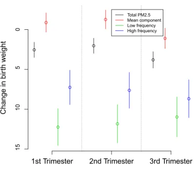
birth weights. Figure 1.2 shows the results from the aforementioned models for the full gestation period, and each of the trimesters.

The results indicate that the effects are fairly similar across trimesters in terms of mag-nitude, direction, and relationship between sources of PM2.5. Both the low and high

frequency components of PM2.5 have large, significantly negative associations on birth

weight suggesting that increased levels of either of these sources adversely affects birth weight. Interestingly the mean component has very small effects, and in the case of trimesters 1 and 2, even slightly positive effects. This would suggest that mothers who gave births during time periods when PM2.5 was elevated had healthier babies in terms

of birth weight. One potential explanation for this effect is that the mean component is confounded by time. We know that this source of PM2.5 represents temporal variation

in exposure. We also know that both PM2.5 and birth weights are decreasing during the

study period, which could explain the slightly positive effect we see. To test this we fit the same model as in 1.23 but included a smooth term for time into the vector of poten-tial confounders,Cij. After applying this model the effect of the mean component drops

down to around -2. By separating out this scale from the low and high frequency scales, we have reduced the possibility of temporal confounding influencing our remaining

(25)

ef-Change in bir th w eight l l l l l l l l l l l l

1st Trimester 2nd Trimester 3rd Trimester

15 10 5 0 Total PM2.5 Mean component Low frequency High frequency

Figure 1.2: Parameter estimates and corresponding 95% confidence intervals from PM2.5

models for each time period. Black line is the estimate of β1 from model 1.22 and the

remaining lines are the estimates ofβ₁∗, β₂∗, β₃∗ from model 1.23

fect estimates as they represent only spatial variability in PM2.5. The effect sizes that we

see for the low and high frequency component are both larger than the overall pollution effect, β1, and this is likely because we have removed the temporal sources of variation

that have smaller effects via the mean component. The effect from the low frequency component seems to be somewhat larger than the high frequency component, though the difference between the two gets smaller across trimesters.

1.5.2 Removing high level information

It is of scientific interest to understand specifically which spatial scales of PM2.5 are

driv-ing changes in birth weight as this will be important in targetdriv-ing future environmental regulations. With that in mind, we repeatedly fit the model with overall pollution, but successively removed high frequency scales from the pollution surface to see how the parameter estimates change. We also keep the mean component separated as the results

(26)

from the previous section indicate that it could be temporally confounded, and leaving it in the term for PM2.5 would dilute the signal that we are seeing from the low and high

frequency components. For a given trimester, the model of interest is now

BWij = ( ˜β0+ ˜β0j) + ˜β1Meanij + ˜β2PMR2.5ij +β˜cCij +ij, (1.24)

noting a couple changes from model 1.22. First we have included the mean component into the model to control for potential sources of temporal confounding. We also have defined a new variable PMR2.5ij, which represents the total pollution with certain spatial

scales removed. PMR2.5ij Always will be missing the mean component for the reasons

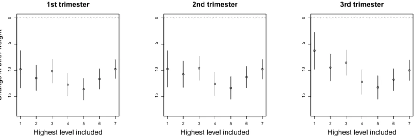
above, and we will further remove the high frequency scales one at at time to see how the effect changes. Figure 1.3 shows the estimates and 95 % confidence intervals from model 1.24 as we remove more and more high frequency information.

The effects show a similar pattern and magnitude among the three different trimesters. We see that removing the highest 1st or 2nd scales from the PM2.5 surface actually

in-creases the magnitude of the effect of PM2.5 on birth weights as the effect goes from -10.0

to -13.2 for the 3rd trimester, with similar jumps in the other trimesters. This suggests that the effects at these very high frequency scales are much smaller in magnitude than their lower frequency counterparts. It is even plausible that these levels could have no effect on birth weight in which case they would represent measurement error and removing them would be a useful feature of our Wavelet decomposition. Looking at the remaining scales we see that there is a decline in effect size as we remove more and more levels, with a large change occurring at scale 4. For trimester 3 the effect drops in magnitude from -12.2 to -8.5 when we exclude the fourth scale from the overall effect. This is a rather large change compared with the other scales and indicates that a source of pollution occurring at that scale has a large impact on birth weights. Overall though the biggest impact seems to occur simply by including the 1st level into the model. The coefficient when we only in-clude the 1st level into the model is -6.23 for trimester 3, and as high as -9.7 for trimesters 1 and 2, indicating that there is a large effect at this scale.

(27)

l l l l l l l 1 2 3 4 5 6 7 15 10 5 0 1st trimester

Highest level included

Change in bir th w eight l l l l l l l 1 2 3 4 5 6 7 15 10 5 0 2nd trimester

l l l l l l l 1 2 3 4 5 6 7 15 10 5 0 3rd trimester

Figure 1.3: Parameter estimates and corresponding 95 % confidence intervals from model 1.24 when we remove high frequency spatial scales for each trimester. Within each panel from right to left we successively remove more and more of the higher frequency scales

1.5.3 Modeling each scale separately

The previous sections lend intuition for which scales are driving the adverse impact of PM2.5on birth weights, but we can also model each individual level separately instead of

clustering them together into a joint exposure. We now fit the following model

BWij = ( ˘β0+ ˘β0j) + ˘β1Meanij + ˘β2Level1+...+ ˘β8Level7+β˘cCij +ij, (1.25)

where we are now including each scale as a separate predictor in the model. The mag-nitude and direction of the coefficients from this model should lend insight into exactly which scales are driving the effects of PM2.5, conditional on the levels of the other scales.

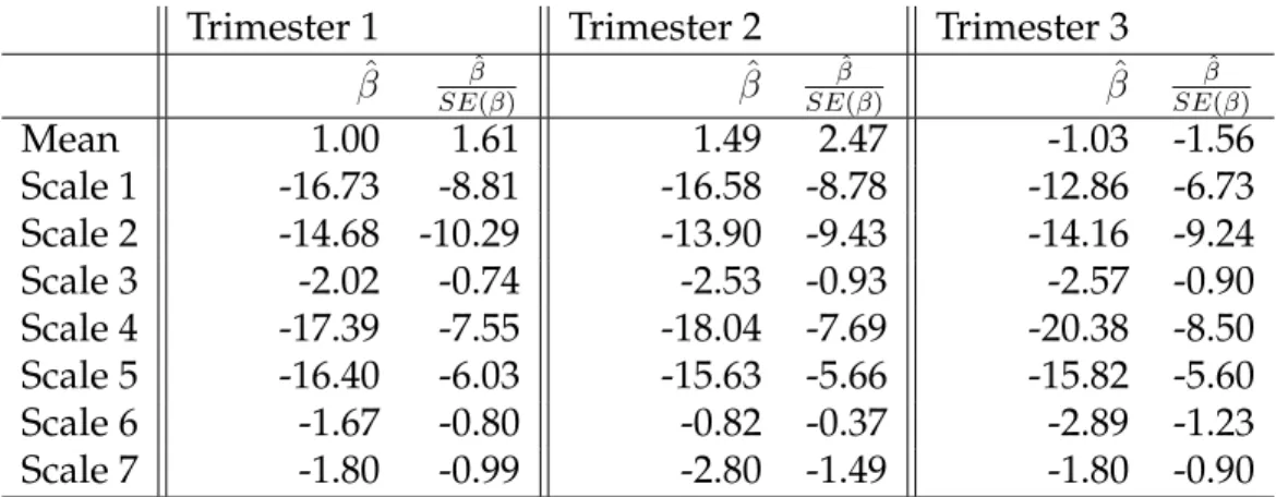
Table 1.1 shows the effect estimates from this model as well as the estimates standard-ized by their standard errors to show the approximate level of significance for each scale. The results generally agree with those seen in figure 1.3 and show a couple of interesting results.

For any trimester, we again see that there is little to no effect of the highest two frequency scales. This further explains why we saw an increase in the magnitude of the overall effect when we removed these scales. Surprisingly, scale 3 seems to have a very small impact on birth weights despite the fact that levels 1, 2, 4, and 5 all have significant impacts on birth weight. The scales are increasing in terms of spatial frequency or the distance at which

(28)

Trimester 1 Trimester 2 Trimester 3 ˆ β _SEβˆ₍_β₎ βˆ _SEβˆ₍_β₎ βˆ _SEβˆ₍_β₎ Mean 1.00 1.61 1.49 2.47 -1.03 -1.56 Scale 1 -16.73 -8.81 -16.58 -8.78 -12.86 -6.73 Scale 2 -14.68 -10.29 -13.90 -9.43 -14.16 -9.24 Scale 3 -2.02 -0.74 -2.53 -0.93 -2.57 -0.90 Scale 4 -17.39 -7.55 -18.04 -7.69 -20.38 -8.50 Scale 5 -16.40 -6.03 -15.63 -5.66 -15.82 -5.60 Scale 6 -1.67 -0.80 -0.82 -0.37 -2.89 -1.23 Scale 7 -1.80 -0.99 -2.80 -1.49 -1.80 -0.90

Table 1.1: Effect estimates from model 1.25

PM2.5changes, so it’s strange to see a spike at one level, and it merits further investigation.

Overall the largest effects of PM2.5 are seen in the first two scales, with significant effects

at scales 4 and 5 as well.

1.5.4 Examination of scales

Due to some interesting results seen in previous sections regarding specific scales of PM2.5

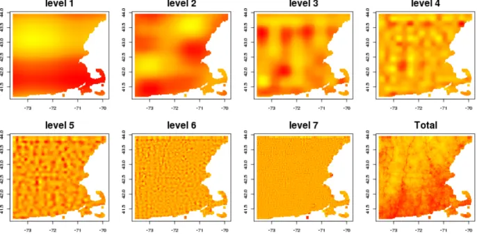
it is of interest to examine these scales further and to be able to translate information from spatial scales to distance, which is more useful to policymakers. We know from sections 1.5.1 - 1.5.3 that scales 1-5 all have significant effects on birth weight with the exception of scale 3, and that the largest such effect sizes seem to come from scales 1, 2, and 4. With this in mind it will be useful to look specifically at these scales and determine what they represent in terms of the PM2.5 surface. Figure 1.4 shows the average surface from

each spatial scale taken by performing our Wavelet decomposition on each day of data in 2006 and averaging them over the 365 days in the year. Visual inspection of these figures coupled with our knowledge of the Massachusetts area allows us to gain intuition as to which sources of pollution each scale is picking up. The first scale seems to pick up some regional transport pollution that is known move from west to east across lower Massachusetts, while the second scale picks up on some slightly noisier effects including the urban background from Boston. The remaining levels are less obvious from the figure, though it does seem that both the 6th and 7th scales are just random noise as postulated from our modeling results as they don’t seem to correlate spatially in any way. We noticed

(29)

earlier that the 3rd scale didn’t seem to have an effect on birth weight and while it is unclear what sources of pollution are driving this scale, it does seem that most of the signal at scale 3 lies in areas where very few people live. This could be what is keeping this scale from having an effect on birth weight.

Figure 1.4: Illustration of average wavelet decomposition averaged over satellite data for 2006. From left to right and top to bottom are the individual scales taken from our wavelet decomposition for each day then averaged over the entire year. The final panel is the sum of all the levels.

It is also of interest to assign a physical distance to each spatial scale as this could be more useful when using these results to consider future air quality regulations. Wavelets in their simplest form, the Haar Wavelet, have a very simple interpretation in terms of distance. The support of the Haar Wavelet at scale 1 is the support of the data, at scale 2 the support is half the length of the data, and this continues as each scale represents a fraction of the data that is half the distance as the previous scale. The Haar Wavelet at any given scale will pickup on features of the function that vary at a level around half of the support of that scale, since the Haar Wavelet is positive for half of it’s support and negative for the other half. While we use the smoother Debauchies family of Wavelet’s that do not have a support that is strictly a fraction of the data, the majority of the support for each scale of the Debauchies Wavelet is splitting up the data into halves. With this in

(30)

mind we can assign to each scale a ’rough’ measure of distance representing the distances at which PM2.5 varies that the particular scale will be accounting for. Since our data

is 302km by 302km, we know that scale 1 represents changes that occur at a distance of around 151km, scale 2 changes at around 75.5, etc. This information along with our results on the impact that each scale has on birth weight could be used in conjunction with scientific expertise to determine what sources of pollution are leading to large, adverse effects on birth weight.

1.6 Discussion

In this article we have proposed a two-dimensional wavelet decomposition that is flex-ible, easy to implement, and scalable to large spatial surfaces. By extending ideas from Wand et al. (2011) we have created a decomposition that does not rely on many of the as-sumptions of standard wavelet theory that are overly restrictive for many analyses, and places the decomposition in a regression framework which simplifies it’s implementation and estimation of wavelet coefficients. Our proposed method will allow researchers to perform multiresolution analyses on spatial data regardless of the structure and scale of their data. Much of the wavelet literature relies on complicated algorithms to perform analyses, but in this paper we simplified wavelet analyses by showing that they are sim-ply basis functions and therefore can be applied in much the same way as any other basis function used to represent a function. We showed in section 1.3 that once we have de-fined and evaluated the wavelet basis functions and placed them in their appropriate design matrix, then estimation is trivial and no different than any other basis function placed in a regression framework. We have found that the proposed method scales quite well as the surfaces of PM2.5 we examined contained approximately 70,000 grid points.

Using 7 wavelet levels we are left with 214 _{= 16}_,₃₄₈ _{basis functions and therefore the}

only computational challenge is in fitting a regression model with a design matrix whose dimensions are 70,000 by 16,384. If the dimensions get too large, we suggest doing an approximation to our method that is based on the fact that the wavelet levels are orthog-onal. One could fit the same regression model, but only include the first 4 to 5 levels

(31)

instead of 7 levels, making the model much faster to calculate. Then the residuals from this model can be regressed against the remaining levels to obtain an approximation to the full wavelet decomposition.

We illustrated our method on a 1km by 1km grid of PM2.5 data and then examined how

these different spatial scales impacted birth weight in Massachusetts. We noticed that the temporal component of PM2.5 was positive or close to zero for each trimester, which is

unexpected as we expect PM2.5 to have a negative effect on birth weight. One potential

explanation for this is confounding by time as both PM2.5and birth weights are decreasing

over time, and therefore leaving time out of the model could lead to misleading effects. We ran further models that included a smooth function of time to eliminate any potential confounding by time and found that the effects of the mean component decreased to negative levels that were expected a priori. We also saw the effect of the low frequency pollution component is larger than the high frequency, though this difference decreases later on in the pregnancy. It is clear though that both have large, negative impacts on birth weight. We also examined the effect of each spatial scale by removing one scale at a time from PM2.5 and seeing how the effect estimate changed. We noticed that the very

high frequency component, which was represented by the 6th and 7th scales, seems to be just noise and is actually attenuating the effect towards zero. It is believed that there is some noise in the AOD measurements that are used to model PM2.5on the 1km grid and

it is possible that the top levels of the wavelet decomposition are picking up solely on this noise. Wavelets have been used to de-noise signals and this de-noising property might be increasing the magnitude of our effects because it is eliminating measurement error which would attenuate the effect to zero. We also noticed that the majority of the effect of PM2.5 is driven by scales 1 through 5 and with the largest effects coming from scales 1

and 4. These results could be very important for future regulations as they can be used to target sources of pollution that operate on those spatial scales.

One limitation of the results from the study of birth weights is that we are ignoring the fact that the PM2.5 measurements are estimated and therefore come with some

uncer-tainty. The confidence intervals placed on our model estimates are under the assumption that PM2.5is a fixed, known quantity and therefore these intervals are likely to be slightly

(32)

anti-conservative. While we are not attempting to make causal statements or statements of significance, rather simply trying to learn about the general magnitude and direction of effects, it would still be ideal to be able to account for this increase in uncertainty. Resam-pling methods could in theory be used to solve this problem, however, that would require resampling and re-fitting of the models used to estimate the exposure and this would not be feasible in this study. A related limitation is that because we are using estimates of PM2.5 there might be measurement error biasing the results of our study. While we

hy-pothesized that we were removing some of the effects of measurement error when we removed the highest two frequency wavelet scales, it’s possible that measurement error is still systematically degrading our model estimates. Future work could focus on ap-plying well developed measurement error correction techniques to examine if the effect estimates are drastically impacted.

As this is one of the first papers trying to separate the effects of different sources of air pollution, there are a vast number of possibilities for future research. One such idea is to use the wavelet decompositions of PM2.5to learn more about specific chemicals that make

up PM2.5. Data is available at monitoring sites about the specific components that PM2.5is

comprised of, which means that we can perform canonical correlation analysis between our 1km decompositions and the component monitoring data to learn about what type of sources each component comes from. This could also lead to information about which components of pollution are negatively impacting health outcomes. It would also be of interest to apply these decompositions to a wide variety of health outcomes to identify if there are any outcomes in which only the local or regional sources of pollution have an effect. It is also of interest to apply more meaningful definitions to each scale. Wavelet scales themselves are not very interpretable, but we can potentially assign to each wavelet level a distance corresponding to the frequency of that level. This would be a much more meaningful interpretation to researchers in environmental health looking to relate these results back to their analyses.

(33)

The positive effects of population based preferential

sampling in environmental epidemiology

Joseph Lawrence Antonelli

Department of Biostatistics

Harvard Graduate School of Arts and Sciences

Luke Bornn

Department of Statistics

Harvard University

Matthew Cefalu

RAND Corporation

(34)

2.1 Introduction

In the past few decades, numerous epidemiological studies have investigated the health effects of air pollution. Many studies have found statistically significant associations be-tween ambient levels of air pollution and a variety of adverse health outcomes. Examples of such studies can be found in Dockery et al. (1993); Samet et al. (2000); Dominici et al. (2006) and a review of the literature can be seen in Dominici et al. (2003); Pope III (2007); Breysse et al. (2013). Difficulty in these studies arises due to spatial misalignment of the data as the locations of the subjects does not coincide with the locations at which we can observe air pollution levels. Most studies rely on monitoring data such as the IMPROVE network or the EPA’s Air Quality System, which are only available at a fixed set of lo-cations. Then, conditional on the monitors, investigators predict values of air pollution using nearest neighbor, kriging, or land use regression approaches (Oliver and Webster, 1990; Madsen et al., 2008; Kloog et al., 2012). In many instances the locations of these monitors are chosen for a specific reason such as measuring areas of high pollution levels or areas of high pollution density. Chow et al. (2002) discuss different designs by which monitoring sites can be chosen and potential objectives for monitor selection, many of which depend on the nature of the pollution itself. Kanaroglou et al. (2005) develop a for-mal method for selecting monitor locations that takes into account the spatial variability of the surface to be estimated, and the population being exposed to pollution. Matte et al. (2013) discuss the how monitor placement in New York City was designed to capture intra-urban spatial variability of air pollution. These are among the many of instances just in exposure estimation where monitors were placed in areas with regard to the lev-els of pollution and therefore is a relevant issue when utilizing these networks in health effect studies.

Numerous papers have been published regarding two stage analyses in environmental applications. The first stage consists of estimating parameters of an exposure model us-ing monitorus-ing data. The second stage then conditions on the exposure estimates from the first stage and uses this estimated exposure to investigate the association between expo-sure and an outcome. This leads to a complex form of meaexpo-surement error, which does not

(35)

fall specifically into the category of either classical or berkson measurement error. Kim et al. (2009) looked at the impact of various predicted exposures on health effect estima-tion in air polluestima-tion studies. A variety of methods have been proposed to correct for this measurement error. Gryparis et al. (2009) examined the effectiveness of a variety of stan-dard correction methods via simulation and gave intuition for when these measurement error corrections will work. More recently, Szpiro et al. (2011b) show that the measure-ment error can be decomposed into two components: A classical like and a berkson like component. They further came up with a computationally efficient form of the paramet-ric bootstrap to correct for measurement error in two stage analyses. Szpiro and Paciorek (2013) take an in depth look at the impact of these two components of measurement error, and derive asymptotic results about the bias and variance of health effect estimates. In this paper our focus will be the preferential sampling of monitors in two stage analyses, and the subsequent impact on measurement error and health effect estimation. Preferen-tial sampling as defined by Diggle et al. (2010) is the scenario where the location of the monitors is dependent on the values of the spatial process they are measuring. In air pol-lution studies this would amount to monitors being placed in locations due to the amount of air pollution in those locations. Diggle et al. (2010) show that variogram estimates are biased under preferential sampling and come up with a method to control for preferen-tial sampling in geostatistical inference. Gelfand et al. (2012) showed that preferenpreferen-tial sampling can perform drastically worse with respect to estimating a spatial surface than sampling under complete spatial randomness (CSR). Interestingly, Szpiro et al. (2011a) show that better exposure prediction doesn’t always lead to improved health effect infer-ence, though in general we expect that improving exposure prediction will lead to better inference overall. Lee et al. (2015) examine the impacts of preferential sampling on health effect estimation in environmental epidemiology and find that the locations of monitors can drastically impact inference in second stage analyses. They also illustrate in a sim-ulation study how inference in the second stage is improved under CSR compared with preferential sampling.

It is clear from the literature that from a strictly geostatistical perspective, preferential sampling can lead to poorer inference and must be accounted for in the exposure

(36)

model-ing process. The aim of this paper, however, is to show that if interest lies in the second stage health effect estimates then preferential sampling can lead to improved inference in many scenarios. The main reason for this and the key difference in our paper with previ-ous studies regarding preferential sampling is that we will be emphasizing the relation-ship that population density plays when thinking about potential locations of monitors. Our results will illustrate the claim made in Szpiro and Paciorek (2013) that the densi-ties governing the location of the subjects and the monitors should be the same. We will show that when taking population density into account, preferential sampling can lead to drastically improved inference in air pollution studies. The outline of our paper is as follows: Section 2.2 will introduce the motivating example of PM2.5in New England,

Sec-tion 2.3 introduces notaSec-tion and the modeling framework, in secSec-tion 2.4 we derive some mathematical results regarding inference under two stage sampling designs, section 2.5 presents an illuminating simulation study to shed light on different aspects of the esti-mation procedure, section 2.6 highlights these results in the context of PM2.5 monitoring

locations in New England, and section 2.7 concludes with a discussion.

2.2 Motivating example

The majority of the preceding discussion and previous work on measurement error in environmental two stage analyses has been motivated by studying the adverse health ef-fects of PM2.5. PM2.5 is a pollutant defined as the combination of all fine particles less

than 2.5 micrometers in diameter. Nearly all research to date on the associations between PM2.5 and health outcomes has been contingent on monitors to estimate exposure, with

the lone exception being recent studies that have used aerosol optical depth (AOD) to estimate PM2.5on a finer grid (Kloog et al., 2012). Generally exposure is estimated

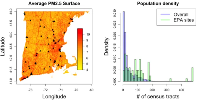
condi-tional on monitoring data, and little attention is paid to the location of the monitors. The left panel in figure 2.1 shows a map of the EPA AQS monitor locations over New England as well as a map of estimated PM2.5 across New England. The estimated PM2.5 for New

England is taken from the aforementioned models that use AOD to estimate exposure on a fine grid, which in this case is 1km by 1km. Looking at figure 2.1 helps to show the

(37)

mo-tivation for this work as it seems from the figure that there are more monitors in areas of higher pollution. It should also be noted that these areas of higher pollution correspond to higher population densities, for instance the right side of the map represents elevated pollution in the greater Boston metropolitan area. The right panel of figure 2.1 further illustrates that the monitor locations are in fact concentrated in more populated areas. As a measure of population density we use the number of census tracts within 0.3 degrees latitude or longitude of a location, and the monitor locations generally have more census tracts nearby than New England as a whole.

Although not definitive, it seems plausible that the location of monitors in New Eng-land follows a non-random sampling scheme, which meets our criteria for preferential sampling. If we are able to gain intuition about the impact of preferential sampling, we should also gain knowledge on how inference is impacted in studies of PM2.5that use the

EPA AQS monitoring system.

Figure 2.1: The left hand panel shows the average predicted PM2.5 surface in New

Eng-land for the year 2003, with the black points representing the location of the EPA AQS monitoring system. The right hand panel shows a histogram of the number of census tracts within 0.3 degrees of each grid point in New England, along with the histogram of the number of census tracts within 0.3 degrees of the EPA monitoring sites

(38)

2.3 General setup

2.3.1 Notation and model

For convenience, we adopt similar notation to Gryparis et al. (2009); Szpiro et al. (2011b); Lee et al. (2015). Throughout we will havensubjects in the study (second stage of anal-ysis), andn∗ monitors at which we observe exposure (first stage of analysis). We define X to be the true exposure at the n subject locations, andX∗ to be the exposure at then∗

monitor locations. In general we will allow the following to hold:

X X∗ ∼N µX(α) µX∗(α) , ΣX,X(φ) ΣX,X∗(φ) ΣX∗_,X(φ) Σ_X∗_,X∗(φ) (2.1) Where µX(α) represents the mean of the exposure surface, and is a linear function of a

set of covariates dictated by a parameter vector,α. The covariance matrix of this Normal distribution is dictated by a parameter vector, φ, which includes standard parameters such as the range, smoothness parameter, etc. This framework is general and allows for a broad class of exposure models for predicting exposure at new locations such as kriging and land use regression. We now define our outcome model as

Y =β0+Xβ1+ (2.2)

Where is a vector of i.i.d random noise. In general this model can include a vector of covariates, though we keep it simple here to simplify results about the parameter of interest,β1. In any realistic scenario, we will not observe X and therefore must estimate X

with W defined as

W =E(X|X∗,α,ˆ φˆ) (2.3) In this situation above, this expectation is easily written out using properties of Normal distributions as

(39)

and the remainder of this paper will examine the impact of using W in place of X in the outcome model, more specifically the impact of that measurement error under different sampling schemes for monitoring locations.

2.3.2 Definition of preferential sampling

In Diggle et al. (2010) preferential sampling is defined as any dependence between the values of the underlying spatial process (X∗in our setting) and the locations at which we observe the process (the monitors in our setting). Mathematically this can be written as

p(X∗, S∗)6=p(X∗)p(S∗), (2.5) where S∗ is a random variable to denote the locations at which we observeX∗. An ex-ample of this would be a network of monitors that are placed to measure high levels of a given process. Most geostatistical procedures assume independence between these two quantities and therefore likelihood based inference in the presence of preferential sampling can lead to bias as the likelihood is misspecified and estimates are no longer assured to be consistent. In their paper they introduce preferential sampling by allow-ing their locations to be drawn from an inhomogeneous Poisson process of the followallow-ing form

λ(S∗) =exp(γ0+γ1X∗), (2.6)

where preferential sampling is the scenario whenγ1 6= 0. Lee et al. (2015) also introduce

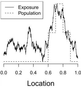
preferential sampling of monitors in their simulations by drawing locations from an in-homogeneous Poisson process whose intensity function depends on observed covariates and unobserved spatial features of the process. We will define preferential sampling in a related, though slightly different way, which we feel is illuminating for studies involving predicted air pollution from monitors. We will investigate scenarios in which sampling depends on the population density with which subjects in the second stage model are drawn from. This can be written as

(40)

P(S, S∗)6=P(S)P(S∗) (2.7) where S now denotes the locations at which we observe subjects from the second stage analysis. This does not strictly imply preferential sampling as defined in equation 2.5, though it will meet that criteria for preferential sampling if the population density is as-sociated with the exposure surface. We saw in section 2.2 that the location of monitors appeared non-random and it seemed that there were more monitors in areas that have both a higher population density and higher pollution levels. The reason for defining preferential sampling in this paper as being related to population density is that this sce-nario commonly occurs in air pollution epidemiology and the extent to which it affects inference is unclear. Previous studies have shown the negative impact that preferential sampling can have on estimation of variograms or other features of the process, however, the main interest in air pollution epidemiology is the second stage outcome model that uses predictions of the process from the first stage modeling.

2.4 Understanding bias and variance of

β

ˆ

₁

We now take a step back to provide mathematical justification for our claim that prefer-ential sampling can improve estimation in two stage analyses of air pollution. We will focus on results regarding β1 as this is the parameter of interest in most environmental

epidemiology studies examining the effect of PM2.5 on a health outcome. We will use the

same notation as before and defineCito be the vector of covariates for subject i, andCj∗to

be the vector of covariates for monitor j. As a simplifying assumption we assume that the joint distribution of all the necessary quantities (Y, X, X∗, C, C∗) follows a multivariate normal distribution, as this will simplify some of the algebraic operations. We further impose the following models:

Y =β0+Xβ1+ (2.8)

(41)

X∗ =C∗α+∗_x (2.10) Whereis a mean zero vector of i.i.d noise, andxandx∗ are mean zero vectors of noise. Notice that we do not impose any independence assumptions aboutx and x∗ allowing for spatial structure in the residuals. Conditional on the estimatesαˆand φˆfrom the first stage analysis, we estimate exposure via equation 2.4. Our interest lies in the distribution ofβˆ1, the estimate ofβ1 we get in the second stage of the model when we use W instead

of X.

2.4.1 Bias of

β

ˆ

1

To examine the bias we can look at the conditional distribution of Y given W. Since we defined everything to be jointly normal, the joint distribution of Y and W can we written as Y W ∼N µy µw , σ_y2 σyw σyw σw2 (2.11) Which leads to Y|W ∼N µy + σyw σ2 w (W −µw), σy2− σyw σ2 w (2.12) The coefficient of interest is the one that lies in front of W in the mean component of the above conditional distribution. Using this fact and definingθ = [α, φ]we can say that

E( ˆβ1) = σyw σ2 w =β1 cov(X, W) V ar(W) =f(ˆθ) (2.13)

and details of this derivation as well as the exact expression forf(ˆθ)can be found in the appendix. One important thing to note is that whenθˆ=θthenf(ˆθ) =β1and there exists

(42)

if we knew the true parameters from the exposure model then we would get an unbiased estimate ofβ1 in the outcome model. To gain more intuition into this bias we can perform

a taylor series expansion off(ˆθ)aroundf(θ).

f(ˆθ)−f(θ)≈ ∂f(θ) ∂θ (ˆθ−θ) + 1 2(ˆθ−θ) T∂ 2_f₍_θ₎ ∂θ∂θT(ˆθ−θ) (2.14)

and now we can take the expectation on both sides with respect to the distribution gov-erning the monitoring locations. Denoting these expectations byES∗()we see that

ES∗ f(ˆθ)−f(θ)=ES∗( ˆβ₁−β₁) ≈ ∂f(θ) ∂θ ES∗(ˆθ−θ) + 1 2T r ∂2_f₍_θ₎ ∂θ∂θT V arS∗(ˆθ−θ) + 1 2ES∗(ˆθ−θ) T∂2f(θ) ∂θ∂θTES∗(ˆθ−θ) (2.15)

So we’ve shown that the unconditional bias (no longer conditional on an estimate ofθ) is a function of the bias and variance ofθˆ.

2.4.2 Variance of

β

ˆ

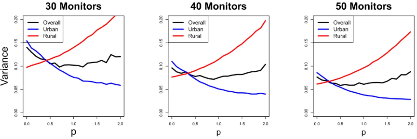
1

To gain intuition into the variance of βˆ1 we can look at var(X−W), the variance of the

measurement error. While this does not translate directly into the variance ofβˆ1, it is well

understood that increasing the amount of measurement error in an exposure will lead to increased variance in the effect of that exposure on the outcome, regardless of the form of the measurement error. To better understand this quantity we can assume that we know the true model parameters and without loss of generality that the mean of the exposure is zero. We will also write our estimated exposure in a somewhat more general way as

W = Pn∗

i=1wiX

∗

i, where the weightswi are a function of the distance betweenX and Xi∗

and sum to one. We can write the variance as

var(X−W) =var(X−

n∗ X

i=1

Statistical Methods for Analyzing Complex Spatial and Missing Data

Statistical Methods for Analyzing

Complex Spatial and Missing Data

The Harvard community has made this

article openly available. Please share how

this access benefits you. Your story matters

Statistical methods for analyzing complex spatial

and missing data

A dissertation presented

by

Joseph Lawrence Antonelli

to

The Department of Biostatistics

in partial fulfillment of the requirements

for the degree of

Doctor of Philosophy

in the subject of

Biostatistics

Harvard University

Cambridge, Massachusetts

September 2015

Statistical methods for analyzing complex spatial

and missing data

Abstract

Contents

Acknowledgments

Spatial multiresolution analysis of irregularly spaced grids

with application to the effect of PM

on birth weights

Joseph Lawrence Antonelli

Department of Biostatistics

Harvard Graduate School of Arts and Sciences

Joel Schwartz

Department of Biostatistics

Harvard Chan School of Public Health

Itai Kloog

The Department of Geography and Environmental Development

Ben-Gurion University of the Negev

Brent Coull

Department of Biostatistics

1.1

Introduction

1.2

PM

and Birthweights in Massachusetts

1.2.1

Exposure data

1.2.2

Birth weights

1.3

Wavelet decomposition for irregular grids

1.3.1

Standard wavelet analysis

1.3.2

One dimensional penalized wavelets

1.3.3

Standard two dimensional wavelets

1.3.4

Two dimensional penalized wavelets

1.4

Application to satellite PM

data

1.5

Analysis of birth weight data

1.5.1

Low vs High frequency components

1.5.2

Removing high level information

1.5.3

Modeling each scale separately

1.5.4

Examination of scales

1.6

Discussion

The positive effects of population based preferential

sampling in environmental epidemiology

Joseph Lawrence Antonelli

Department of Biostatistics

Harvard Graduate School of Arts and Sciences

Luke Bornn