This document is confidential and is proprietary to the American Chemical Society and its authors. Do not copy or disclose without written permission. If you have received this item in error, notify the sender and delete all copies.
Prediction errors of molecular machine learning models lower than hybrid DFT error
Journal: Journal of Chemical Theory and Computation
Manuscript ID ct-2017-00577j.R1 Manuscript Type: Article
Date Submitted by the Author: 19-Sep-2017
Complete List of Authors: Faber, Felix; University of Basel Hutchison, Luke; Google
Huang, Bing; University of Basel Gilmer, Justin; Google
Schoenholz, Samuel; Google Dahl, George; Google Vinyals, Oriol; Google Kearnes, Steven; Google Riley, Patrick; Google
von Lilienfeld, O. Anatole; University of Basel
Prediction errors of molecular machine
learning models lower than hybrid DFT error
Felix A. Faber,
†,§Luke Hutchison,
‡,§Bing Huang,
†Justin Gilmer,
‡Samuel S.
Schoenholz,
‡George E. Dahl,
‡Oriol Vinyals,
¶Steven Kearnes,
‡Patrick F. Riley,
‡and O. Anatole von Lilienfeld
∗,††Institute of Physical Chemistry and National Center for Computational Design and Discovery of Novel Materials, Department of Chemistry, University of Basel,
Klingelbergstrasse 80, CH-4056 Basel, Switzerland
‡Google, 1600 Amphitheatre Parkway, Mountain View, CA, US - 94043 CA
¶Google, 5 New Street Square, London EC4A 3TW, UK
§Authors contributed equally
E-mail: [email protected]
Abstract
We investigate the impact of choosing regres-sors and molecular representations for the con-struction of fast machine learning (ML) models of thirteen electronic ground-state properties of organic molecules. The performance of each re-gressor/representation/property combination is assessed using learning curves which report out-of-sample errors as a function of training set size with up to ∼118k distinct molecules. Molecu-lar structures and properties at hybrid density functional theory (DFT) level of theory come from the QM9 database [Ramakrishnan et al,
Scientific Data 1 140022 (2014)] and include
enthalpies and free energies of atomization , HOMO/LUMO energies and gap, dipole mo-ment, polarizability, zero point vibrational en-ergy, heat capacity and the highest fundamental vibrational frequency. Various molecular repre-sentations have been studied (Coulomb matrix, bag of bonds, BAML and ECFP4, molecular graphs (MG)), as well as newly developed dis-tribution based variants including histograms of distances (HD), and angles (HDA/MARAD), and dihedrals (HDAD). Regressors include lin-ear models (Bayesian ridge regression (BR) and linear regression with elastic net
regu-larization (EN)), random forest (RF), kernel ridge regression (KRR) and two types of neural networks, graph convolutions (GC) and gated graph networks (GG). Out-of sample errors are strongly dependent on the choice of rep-resentation and regressor and molecular
prop-erty. Electronic properties are typically best accounted for by MG and GC, while energetic properties are better described by HDAD and KRR. The specific combinations with the low-est out-of-sample errors in the ∼118k training set size limit are (free) energies and enthalpies of atomization (HDAD/KRR), HOMO/LUMO eigenvalue and gap (MG/GC), dipole moment (MG/GC), static polarizability (MG/GG), zero point vibrational energy (HDAD/KRR), heat capacity at room temperature (HDAD/KRR), and highest fundamental vibrational frequency (BAML/RF). We present numerical evidence that ML model predictions deviate from DFT (B3LYP) less than DFT (B3LYP) deviates from experiment for all properties. Furthermore, out-of-sample prediction errors with respect to hybrid DFT reference are on par with, or close to, chemical accuracy. The results suggest that ML models could be more accurate than hybrid DFT if explicitly electron correlated quantum (or experimental) data was available.
1
ACS Paragon Plus Environment
1 2 3 4 5 6 7 8 9 10 11 12 13 14 15 16 17 18 19 20 21 22 23 24 25 26 27 28 29 30 31 32 33 34 35 36 37 38 39 40 41 42 43 44 45 46 47 48 49 50 51 52 53 54 55 56 57 58 59 60
1
Introduction
Due to its favorable trade-off between accuracy and computational cost, Density Functional Theory (DFT)1,2 is the workhorse of
quan-tum chemistry3—despite its well known
short-comings regarding spin-states, van der Waals interactions, and chemical reactions.4,5
Fail-ures to predict reaction profiles are particu-larly worrisome,6 and recent analysis casts even
more doubts on the usefulness of DFT func-tionals obtained through parameter fitting.7
The prospect of universal and computation-ally much more efficient machine learning (ML) models, trained on data from experiments or generated at higher levels of electronic structure theory such as post-Hartree Fock or quantum Monte Carlo (e.g. exemplified in Ref.8),
there-fore represents an appealing alternative strat-egy. Not surprisingly, a lot of recent effort has been devoted to developing ever more accurate ML models of properties of molecular and con-densed phase systems.
Several ML studies have already been pub-lished using a data set called QM9,9
consist-ing of molecular quantum properties for the ∼134k smallest organic molecules containing up to 9 heavy atoms (C, O, N, or F; not counting H) in the GDB-17 universe.10 Some
of these studies have developed or used rep-resentations we consider in this work, such as BAML (Bonds, angles, machine learning),11
bag of bonds (BOB)12,13 and the Coulomb
ma-trix (CM).13,14Atomic variants of the CM have
also been proposed and tested on QM9.15Other
representations have also been benchmarked on QM9 (or QM7 which is a smaller but simi-lar data set), such as Fourier series of radial distance distributions,16 motifs,17 the smooth
overlap of atomic positions (SOAP)18 in
com-bination with regularized entropy match,19
con-stant size descriptors based on connectivity and encoded distance distributions.20
Ramakrish-nan et al.8 introduced a∆-ML approach, where
the difference between properties calculated at coarse/accurate quantum level of theories is being modeled. Furthermore, neural network models, as well as deep tensor neural networks, have recently been proposed and tested on the
same or similar data sets.21,22 Dral et al.23 use
such data to machine learn optimal molecule specific parameters for the OM224
semiempir-ical method, and orthogonalization tests are benchmarked in Ref.25
However, limited work has yet been done in systematically assessing various methods and
properties on large sets of the exact same chem-icals.26 In order to unequivocally establish if
ML has the potential to replace hybrid DFT for the screening of properties, one has to demonstrate that ML test errors are system-atically lower than estimated hybrid DFT ac-curacies for all the properties available. This study accomplishes that through a large scale assessment of unprecedented scale: (i) In or-der to approximate large training set sizes
N, we included 13 quantum properties from
up to ∼118k molecules in training (90% of QM9). (ii) We tested multiple regressors (Bayesian ridge regression (BR), linear regres-sion with elastic net regularization (EN), ran-dom forest (RF), kernel ridge regression (KRR), neural network (NN) models graph convolu-tions (GC)27 and gated graphs (GG)28) and
(iii) multiple representations including BAML, BOB, CM, extended connectivity fingerprints (ECFP4), histograms of distance, angle, and dihedral (HDAD), molecular atomic radial an-gular distribution (MARAD), and molecular graphs (MG). (iv) We investigated all
combi-nations of regressors and representations, ex-cept for MG/NN which was exclusively used together because GC and GG depend funda-mentally on the input representation being a graph instead of a flat feature vector.
The best models for the various proper-ties are: atomization energy at 0 Kelvin (HDAD/KRR), atomization energy at room temperature (HDAD/KRR), enthalpy of atom-ization at room temperature (HDAD/KRR), atomization of free energy at room tempera-ture (HDAD/KRR), HOMO/LUMO eigenvalue and gap (MG/GC), dipole moment (MG/GC), static polarizability (MG/GG), zero point vi-brational energy (HDAD/KRR), heat capac-ity at room temperature (HDAD/KRR), and the highest fundamental vibrational frequency (BAML/RF). For training set size of ∼118k
1 2 3 4 5 6 7 8 9 10 11 12 13 14 15 16 17 18 19 20 21 22 23 24 25 26 27 28 29 30 31 32 33 34 35 36 37 38 39 40 41 42 43 44 45 46 47 48 49 50 51 52 53 54 55 56 57 58 59 60
(90% of data set) we have found the additional out-of-sample error added by machine learning to be lower or as good as DFT errors at B3LYP level of theory relative to experiment for all properties, and that chemical accuracy (See ta-ble 3) is reached, or in sight.
This paper is organized as follows: First we will briefly describe the methods, includ-ing data set, model validation protocols, rep-resentations, and regressors. In section III, we present the results and discuss them, and sec-tion IV concludes the paper.
2
Method
2.1
Data set
We have used the QM9 data set consisting of ∼134k drug-like organic molecules.9 Molecules
in the data set consist of H, C, O, N and F, and contain up to 9 heavy atoms. For each molecule several properties, calculated at DFT level of theory (B3LYP/6-31G(2df,p)), were included. We used: Atomization energy at 0 Kelvin U0
(eV); atomization energy at room temperature
U (eV); enthalpy of atomization at room
tem-perature H (eV); atomization of free energy
at room temperature G (eV); HOMO
eigen-value εHOMO (eV); LUMO eigenvalue εLUMO
(eV); HOMO-LUMO gap ∆ε (eV); norm of
dipole momentµ=qP
r∈x,y,z(
R
drn(r)r)2
(De-bye), where n(r) is the molecular charge
den-sity distribution; static isotropic polarizability
α = 1 3
P
i∈x,y,zαii (Bohr
3), where
αii is the
di-agonal element of the polarizability tensor; zero point vibrational energy ZPVE (eV); heat ca-pacity at room temperature Cv (cal/mol/K);
and the highest fundamental vibrational fre-quency ω1 (cm−1). For energies of atomization
(U0, U, H and G) all models yield very
sim-ilar errors. We will therefore only discuss U0
for the remainder. The 3053 molecules speci-fied in Ref.9 which failed SMILES consistency
tests were excluded from our study, as well as two linear molecules, leaving∼131k molecules.
2.2
Model validation
Starting from the ∼131k molecules in QM9 af-ter removing the ∼3k molecules (see above) we have created a number of train-validation-test splits. We have splitted the data set into test and non-test sets and varied the percentage of data in test set to explore the effect of amount of data in error rates. Inside the non-test set, we have performed 10 fold cross validation for hyperparameter optimization. That is, for each model 90% (the training set) of the non-test set is used for training and 10% (the valida-tion set) is used for hyperparameter selecvalida-tion. For each test/non-test split, we have trained 10 models on different subsets of the non-test set, and we report the mean error on the test set across those 10 models. Note that the non-test set will be referred to as training set in the re-sults section in order to simplify discussion.
In terms of CPU investments necessary for training the respective models we note that EN/BR, RF/KRR, and GC/GG required min-utes, hours, and multiple days, respectively. Using GPUs could dramatically reduce such timings.
2.3
DFT errors
To place the quality of our prediction er-rors in the right context, experimental accu-racy estimates of hybrid DFT become desir-able. Here, we summarize literature results comparing DFTat B3LYP level of theory to
ex-periments for the various properties we study. Where data is available, the corresponding de-viation from experiment is listed in Table 3, alongside our ML prediction errors (vide infra).
In order to also get an idea of hybrid DFT energy errors for organic molecules, such as the compounds studied herewithin, we refer to a comparison of PBE and B3LYP results for 6k constitutional isomers of C7H10O2.8 After
cen-tering the data by subtracting their mean shift from G4MP2 (177.8 (PBE) and 95.3 (B3LYP) kcal/mol). The remaining MAEs are roughly ∼2.5 and ∼ 3.0 kcal/mol for B3LYP and PBE, respectively. This is in agreement with what Curtiss et al.29 found. They compared DFT
3
ACS Paragon Plus Environment
1 2 3 4 5 6 7 8 9 10 11 12 13 14 15 16 17 18 19 20 21 22 23 24 25 26 27 28 29 30 31 32 33 34 35 36 37 38 39 40 41 42 43 44 45 46 47 48 49 50 51 52 53 54 55 56 57 58 59 60
to experimental values from 69 small organic molecules (of which 47 were substituted with F, Cl, and S), with up to 6 heavy atoms (not counting hydrogens), and calculated the ener-gies using B3LYP/6-311+G(3df,2p). The re-sulting mean absolute deviation from experi-mental values was 2.3 kcal/mol.
Rough hybrid DFT error estimates for dipole moment and polarizability have been obtained from Refs.30.The errors are estimated
refer-enced to experimental values, for a data set con-sisting of 49 molecules with up to 7 heavy atoms (C, Cl, F, H, O, P, or S)
Frontier molecular orbital energies (HOMO, LUMO and HOMO-LUMO gap) can not be measured directly. However, for the exact (yet unknown) exchange-correlation potential, the Kohn-Sham HOMO eigenvalues correspond to the negative of the vertical ionization poten-tial (IP).31 Unfortunately, within hybrid DFT,
the precise meaning of the frontier eigenvalues and the gap is less clear, and we therefore re-frain from a direct comparison of B3LYP to experimental numbers. Nevertheless, we have included eigenvalues and the gap due to their widespread use for molecular and materials de-sign applications.
Hybrid DFT RMSE estimates with respect to experimental values of ZPVE andω1 (the
high-est fundamental vibrational frequency) were published in Ref.32 for a set of 41 organic
molecules, with up to 6 heavy atoms (not count-ing hydrogen) and calculated uscount-ing B3LYP/cc-pVTZ.
Normally distributed data has a constant ratio between RMSE and MAE,33 which is
roughly 0.8. We have used this ratio to ap-proximate the MAE from the RMSE estimates reported for ZPVE and ω1. Deviation of DFT
(at the B3LYP/6-311g** level of theory) from experimental heat capacities were reported by DeTar34 who obtained errors of 16 organic
molecules, with up to 8 heavy atoms (not count-ing hydrogens).
Note, however, that one should be cautious when referring to these errors: Strictly speak-ing they can not be compared since different ba-sis sets, molecules, and experiments were used. We also note that all DFT errors in this
pa-per are estimated from B3LYP and using other functionals can yield very different errors.
Nevertheless, we feel that the quoted errors provide meaningful guidance as to what one can expect from DFT for each property.
2.4
Representations
The design of molecular representations is a long-standing problem in chem-informatics and materials informatics, and many interesting and promising variants have already been proposed. Below, we provide the details on the represen-tations selected for this study. While finalizing our study, competitive alternatives were intro-duced35,36 but have been tested only for
ener-gies (and polarizabilities).
2.4.1 CM and BOB
The Coulomb matrix (CM) representation14 is
a square atom by atom matrix, where off diago-nal elements are the Coulomb nuclear repulsion terms between atom pairs. The diagonal ele-ments approximate the electronic potential en-ergy of the free atoms. Atom indices in the CM are sorted by the L1 norm of each atom’s row
(or column). The Bag of Bonds (BOB)12
repre-sentation uses exclusively CM elements, group-ing them for different atom pairs into different bags, and sorting them within each bag by their relative magnitude.
2.4.2 BAML
The recently introduced BAML (Bonds, an-gles, machine learning) representation can be viewed as a many-body extension of BOB.11 All pairwise nuclear repulsions are
re-placed by Morse/Lennard-Jones potentials for bonded/non-bonded atoms respectively. Fur-thermore, three- and four-body interactions between covalently bonded atoms are included using angular and torsional terms, respectively. Parameters and functional forms are based on the universal force field (UFF).37
1 2 3 4 5 6 7 8 9 10 11 12 13 14 15 16 17 18 19 20 21 22 23 24 25 26 27 28 29 30 31 32 33 34 35 36 37 38 39 40 41 42 43 44 45 46 47 48 49 50 51 52 53 54 55 56 57 58 59 60
2.4.3 ECFP4
Extended Connectivity Fingerprints38(ECFP4)
are a common representation of molecules in cheminformatics based studies. They are par-ticularly popular for drug discovery.39–41 The
basic idea, typical also for other cheminfor-matics descriptors42(e.g. thesignature
descrip-tor43,44) is to represent a molecule as the set of
subgraphs up to a fixed diameter (here we use ECFP4, which is a max diameter of 4 bonds). To produce a fixed length vector, the subgraphs can be hashed such that every subgraph sets one bit in the fixed length vector to 1. In this work, we use a fixed length vector of size 1024. Note that ECFP4 is based solely on the molec-ular graph specifying all covalent bonds, e.g. as encoded by SMILES strings.
2.4.4 MARAD
Molecular atomic radial angular distribution (MARAD) is an atomic radial distribution function (RDF) based representation. Per atom it consists of three RDFs using Gaussians of in-teratomic distances, and parallel and orthog-onal projections of distances in atom triplets, respectively. Distances between two molecules can be evaluated analytically. Unfortunately, most regressors evaluated in this work, such as BR, EN and RF, do not rely on inner prod-ucts and distances between representations. We resolve this issue by projecting MARAD onto bins in order to work with all regressors (apart for GG and GC which use MG exclusively). The three body terms in MARAD contain in-formation about both, angles and distances of all atoms involved. This differs from HDA (see below), where distances, and angles are decou-pled, and placed in separated bins. Note that unlike BAML or HDAD, there are only two and three-body terms, no four-body terms (dihedral angles) have been included within MARAD.
Details about how the projected MARAD is calculated can be found under in the Supple-mentary materials.
Further details and characteristics of MARAD will also be discussed in a forthcoming separate in-depth study.
2.4.5 HD, HDA, and HDAD
BOB, BAML and MARAD rely on comput-ing functions for given interatomic distances, and/or angles, and/or torsions, and then either project that value on to discrete bins, or sort the values. As a straightforward alternative, we also investigated representations which account directly from pairwise distances, triple-wise an-gles, and quad-wise dihedral angles through manually generated bins in histograms. The resulting representations in increasing inter-atomic many-body order are called HD (His-togram of distances), HDA (His(His-togram of dis-tances and angles), and HDAD (Histogram of distances, angles and dihedral angles). For any given molecule, one iterates through each atom
ai, producing a set of distances, angle and
di-hedral angle features for ai.
Distance features were produced by
measur-ing the distance between ai and aj (for i 6= j)
for each element pair. The distance features were assigned a label incorporating the atomic symbols ofaiandaj sorted alphabetically (with
H last), e.g. if ai was a carbon atom and aj
was a nitrogen atom, the distance feature for the atom pair would be labeled C-N. These la-bels will be used to group all features with the same label into a histogram and allow us to only count each pair of atoms once.
Angle features were produced by taking the principal angles formed by the two vectors span-ning from each atom ai to every subset of 2 of
its 3 nearest atoms, aj and ak. The angle
fea-tures were labeled by the element type of ai,
followed by the alphabetically sorted element types (Except for hydrogens, which were listed last) of aj and ak. The example where ai is a
Carbon atom, aj a Hydrogen atom,ak a
Nitro-gen would be assigned the label C-N-H.
Dihedral angle features were produced by
tak-ing the principal angles between two planes. We take ai as the origin, and for each of the four
nearest neighbors in turn, labeling the neighbor atom aj, and forming a vector Vij = ai → aj.
Then all 3 2
subsets of the remaining three out of four nearest neighbors of ai are chosen, and
labeled asakandal. This third and fourth atom
respectively form two triangular faces when 5
ACS Paragon Plus Environment
1 2 3 4 5 6 7 8 9 10 11 12 13 14 15 16 17 18 19 20 21 22 23 24 25 26 27 28 29 30 31 32 33 34 35 36 37 38 39 40 41 42 43 44 45 46 47 48 49 50 51 52 53 54 55 56 57 58 59 60
paired withVij: hak, ai, ajiand hal, ai, aji. The
dihedral angle between the two triangular faces was calculated. These dihedral angle features were labeled with the atomic symbol forai,
fol-lowed by the atomic symbols for aj, ak and al,
sorted alphabetically, with the exception that hydrogens were listed last, e.g. C-C-N-H.
The features from all molecules have been ag-gregated for each label type to generate a his-tograms for each label type. Fig. 1 exemplifies this for N distances, C angles, and C-C-C-O dihedrals for the entire QM9 data set. Certain typical molecular characteristics can be recognized upon mere inspection. For example, the CN histogram displays a strong and iso-lated peak between 1.1 and 1.5 Å, correspond-ing to occurrences of scorrespond-ingle, double, and triple bonds. For distances above 2 Å, peaks at typ-ical radii of second and third covalent bonding shells around N can be recognized at 2.6 Å and 3.9 Å. Also C-C-C angles can be easily inter-preted: The peak close to zero and π Rad
cor-responds to geometries where three atoms are part of a linear (alkyne, or nitrile) type of mo-tif. The broad and largest peak corresponds to 120 and 109 degrees, typically observed in sp2
and sp3 hybridized atoms.
The morphology of each histogram has then been examined to identify apparent peaks and troughs, motivated by the idea that peaks indicate structural commonalities among molecules. Bin centers have been placed at each significant local minimum and maximum (Shown as vertical lines in Fig. 1). Values at 15-25 bin centers have been chosen as a rep-resentation for each label type. All bin center values are provided in the Supplementary Ma-terial. For each molecule, the collection of features has subsequently been rendered into a fixed-size representation, producing one vector component for each bin center, within each la-bel type. This has been accomplished following a two-step process. (i) Binning and interpola-tion: Each feature value is projected on the two
nearest bins. The relative amount projected on each bin uses linear projection between the two bins. For example: A feature with value 1.7
which lies between two bins placed at 1.0 and 2.0 respectively, contributes 0.3 and 0.7 to the
first and second bin respectively. (ii)Reduction:
The collection of contributions within each bin of each molecule’s feature vector is condensed to a single value by summing all contributions.
2.4.6 Molecular Graphs
We have investigated several neural network models which are based on molecular graphs (MG) as representation. The inputs are real-valued vectors associated with each atom and with each pair of atoms. More specifi-cally, we have used the featurization described in Kearnes et al.27 with the removal of partial
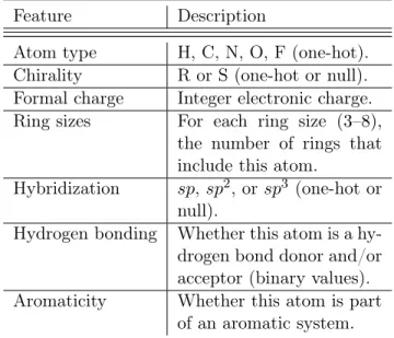
charge and the addition of Euclidean distances to the pair feature vectors. All elements of the feature vector are described in Tables 1 and 2.
The featurization process was unsuccessful for a small number of molecules (367) because of conversion failures from geometry to ratio-nal SMILES string when using OpenBabel45or
RDKit,46and were excluded from all results
us-ing the molecule graph features.
Table 1: Atom features for the MG represen-tation: Values provided for each atom in the molecule.
Feature Description
Atom type H, C, N, O, F (one-hot). Chirality R or S (one-hot or null). Formal charge Integer electronic charge. Ring sizes For each ring size (3–8),
the number of rings that include this atom.
Hybridization sp, sp2, or sp3 (one-hot or null).
Hydrogen bonding Whether this atom is a hy-drogen bond donor and/or acceptor (binary values). Aromaticity Whether this atom is part
of an aromatic system.
Note that within a previous draft of this study,47 we reported biased results for GC/GG
models due to use of Mulliken partial charges within the MG representation. All MG re-sults presented herewithin have been obtained without any Mulliken charges in the represen-tation. Model hyper parameters for the GC
1 2 3 4 5 6 7 8 9 10 11 12 13 14 15 16 17 18 19 20 21 22 23 24 25 26 27 28 29 30 31 32 33 34 35 36 37 38 39 40 41 42 43 44 45 46 47 48 49 50 51 52 53 54 55 56 57 58 59 60
ACS Paragon Plus Environment 1 2 3 4 5 6 7 8 9 10 11 12 13 14 15 16 17 18 19 20 21 22 23 24 25 26 27 28 29 30 31 32 33 34 35 36 37 38 39 40 41 42 43 44 45 46 47 48 49 50 51 52 53 54 55 56 57 58 59 60
logarithmic grid for the 10 percent training set (from 0.25 to 8192 for Gaussian kernel and 0.1 to 16384 for Laplacian kernel). In order to sim-plify the width screening, prior to learning all feature vectors were normalized (scaling the in-put vector by the mean norm across the train-ing set) by the Euclidean norm for the Gaussian kernel and the Manhattan norm for the Lapla-cian kernel.
2.5.2 Bayesian Ridge Regression
We use BR54 as is implemented in
scikit-learn.53 BR is a linear model with aL2 penalty
on the coefficients. Unlike Ridge Regression where the strength of that penalty is a regu-larization hyperparameter which must be set, in Bayesian Ridge Regression the optimal reg-ularizer is estimated from the data.
2.5.3 Elastic Net
Also EN55 is a linear model. Unlike BR, the
penalty on the weights is a mix of L1 and
L2
terms. In addition to the regularization hyper-parameter for the weight penalty, Elastic net has an additional hyperparameter l1_ratio to control the relative strength of the L1 and
L2
weight penalties. We used the scikit-learn53
im-plementation and set l1_ratio = 0.5. We then
did a hyperparameter search on regularizing pa-rameter in a base 10 logarithmic grid from1e−6
to 1.0.
2.5.4 Random Forest
We use RF56 as implemented in scikit-learn.53
RF regressors produce a value by averaging many individual decision trees fitted on ran-domly resampled sets of the training data. Each node in each decision tree is a threshold of one input feature. Early experiments did not reveal strong differences in performance based on the number of trees used, once a minimal number was reached. We have used 120 trees for all regressions.
2.5.5 Graph Convolutions
We have used the GC model as described in Kearnes et al.27, with several structural
mod-ifications and optimized hyperparameters. The graph convolution model is built on the con-cepts of “atom” layers (one real vector asso-ciated with each atom) and “pair” layers (one real vector associated with each pair of atoms). The graph convolution architecture defines op-erations to transform atom and pair layers to new atom and pair layers. There are three structural changes to the model used herewithin when compared to the one described in Kearnes et al.27. We describe these briefly here with
de-tails in the Supplementary Material. First, we have removed the “Pair order invariance” prop-erty by simplifying the (A → P)
transforma-tion. Since the model only uses the atom layer for the molecule level features, pair order in-variance is not needed. Second, we have used the Euclidean distance between atoms. In the (P → A) transformation, we divide the value
from the convolution step by a series of dis-tance exponentials. If the original convolution for an atom pair (a, b) with distance d
pro-duces a vectorV, we concatenate the vectorsV, V d1, V d2, V d3, and V
d6 to produce the transformed
value for the pair (a, b). Third, we have
fol-lowed other work on neural networks based on chemical graphs57 which uses a sum of softmax
operations to convert a real valued vector to a sparse vector and sum those sparse vectors across all the atoms. We use the same oper-ation here along with a simple sum across the atoms to produce molecule level features from the top atom layer. We have found that this works as well or better than the Gaussian his-tograms first used in GC.27 To optimize the
network, we have searched the hyperparame-ter space using Gaussian Process Bandit Op-timization58 as implemented by HyperTune.59
The hyperparameter search has been based on the evaluation of the validation set for a sin-gle fold of the data. Further details including parameters, and search ranges chosen for this paper are listed in the Supplementary materi-als. 1 2 3 4 5 6 7 8 9 10 11 12 13 14 15 16 17 18 19 20 21 22 23 24 25 26 27 28 29 30 31 32 33 34 35 36 37 38 39 40 41 42 43 44 45 46 47 48 49 50 51 52 53 54 55 56 57 58 59 60
2.5.6 Gated Graph Neural Networks
We have used the GG Neural Networks model (GG) as described in Li et al.28. Similar to the
GC model, it is a deep neural network whose input is a set of node features {xv, v ∈G}, and
an adjacency matrixAwith entries in a discrete
set S ={0,1,· · · , k} to indicate different edge types. It has internal hidden representations for each node in the graph ht
v of dimension d
which it updates forT steps of computation. Its
output is invariant to all graph isomorphisms, meaning the order of the nodes presented to the model does not matter. To include the most rel-evant distance information we distinguish four different covalent bonding types (single, double, triple, aromatic). For all remaining atom-pairs we bin them by their interatomic distance [in Å] into 10 bins: [0, 2], [2,2.5], [2.5,3], [3,3.5], [3.5,4], [4,4.5], [4.5,5], [5,5.5], [5.5,6], and [6,∞]. Using these bins, the adjacency matrix has en-tries in an alphabet of size 14 (k=14), indicating bond type for covalently bonded atoms, and dis-tance bin for all other atoms. We have trained the GG model on each target property individ-ually. Further technical details are specified in the Supplementary materials.
3
Results and discussion
3.1
Overview
We present an overview of the most relevant nu-merical results in Table 3. It contains the test errors for all combinations of regressors and rep-resentations and properties for models trained on ∼118 k molecules. The best models for the respective properties are U0 (HDAD/KRR), εHOMO (MG/GC), εLUMO (MG/GC), ∆ε
(MG/GC), µ (MG/GC), α (MG/GG), ZPVE
(HDAD/KRR), Cv (HDAD/KRR), and ω1
(BAML/RF). We do not show results for the other three energies, U(T = 298K), H(T = 298K), G(T = 298K) since identical
observa-tions as forU0 can be made.
Overall, NN and KRR regressors perform well for most properties. The ML out-of-sample errors outperform DFT accuracy at B3LYP level of theory and reach chemical (target)
accuracy, both defined alongside in table 3, for U0 (HDAD/KRR and MG/GG), µ (GC), Cv (HDAD/KRR), and ω1 (BAML/KRR,
MG/GC, HDAD/KRR, BOB/KRR, HD/KRR and MG/GG). For the remaining properties ( εHOMO, εLUMO, ∆ǫ, α, and ZPVE) the best
models come within a factor 2 of target accu-racy, while all (except εHOMO, εLUMO and ∆ǫ)
where we don’t have reliable data. outperform-ing DFT accuracy.
In Fig. 2 out-of-sample errors as a function of training set size (learning curves) are shown for all properties and representations with the best corresponding regressor. It is important to note that all models on display
systemat-ically improve with training set size, exhibit-ing the typical linearly decayexhibit-ing behavior on a log-log plot.11,61 Errors for most models shown
decay with roughly the same slopes, indicat-ing similar exponents in the power-law of error decay. Notable exceptions, i.e. property mod-els with considerably steeper learning curves (Slopes and off-sets of all learning curves can be found in Tables S4 and S5 in the Supplemen-tary Material ), are MG/GC forµ, MG/GG and
HDAD/KRR for α, CM/KRR and BOB/KRR
forhR2i, HDAD/KRR and MG/GG for
U0, and
MG/GG for ω1. These results suggest that
the specified representations capture particu-larly well the effective dimensionality of the cor-responding property in chemical space.
3.2
Regressors
Inspection of Table 3 indicates that the regres-sors can roughly be ordered by performance, independent of property and representation: GC>GG>KRR>RF>BR>EN. It is
notewor-thy how EN, BR, and RF regressors perform substantially worse than GC/GG/KRR. The bad performance of EN and BR is due to their low model capacities. This can also be seen from the learning curves of all regressors presented in Figures S1 to S6 of the Supple-mentary Material. The performance of BR and EN improves only slightly with increased training set size and even gets worse for some property/representation combinations. These two regressors also exhibit very similar learn-9
ACS Paragon Plus Environment
1 2 3 4 5 6 7 8 9 10 11 12 13 14 15 16 17 18 19 20 21 22 23 24 25 26 27 28 29 30 31 32 33 34 35 36 37 38 39 40 41 42 43 44 45 46 47 48 49 50 51 52 53 54 55 56 57 58 59 60
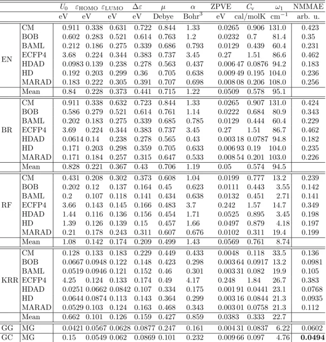
Table 3: MAE on out-of-sample data of all representations for all regressors and properties at∼118k (90%) training set size. Regressors include linear regression with elastic net regularization (EN),
Bayesian ridge regression (BR), random forest (RF), kernel ridge regression (KRR) and molecular graphs based neural networks (GG/GC). The best combination for each property are highlighted in bold. Additionally, the table contains mean MAE of representations for each property and regressor; and normalized, by MAD (See Table 4), mean MAE (NMMAE) over all properties for each regressor/representation combination.
U0 εHOMO εLUMO ∆ε µ α ZPVE Cv ω1 NMMAE eV eV eV eV Debye Bohr3 eV cal/molK cm−1 arb. u.
EN CM 0.911 0.338 0.631 0.722 0.844 1.33 0.0265 0.906 131.0 0.423 BOB 0.602 0.283 0.521 0.614 0.763 1.2 0.0232 0.7 81.4 0.35 BAML 0.212 0.186 0.275 0.339 0.686 0.793 0.0129 0.439 60.4 0.231 ECFP4 3.68 0.224 0.344 0.383 0.737 3.45 0.27 1.51 86.6 0.462 HDAD 0.0983 0.139 0.238 0.278 0.563 0.437 0.006 47 0.0876 94.2 0.183 HD 0.192 0.203 0.299 0.36 0.705 0.638 0.009 49 0.195 104.0 0.236 MARAD 0.183 0.222 0.305 0.391 0.707 0.698 0.008 08 0.206 108.0 0.256 Mean 0.84 0.228 0.373 0.441 0.715 1.22 0.0509 0.578 95.1 BR CM 0.911 0.338 0.632 0.723 0.844 1.33 0.0265 0.907 131.0 0.424 BOB 0.586 0.279 0.521 0.614 0.761 1.14 0.0222 0.684 80.9 0.343 BAML 0.202 0.183 0.275 0.339 0.685 0.785 0.0129 0.444 60.4 0.229 ECFP4 3.69 0.224 0.344 0.383 0.737 3.45 0.27 1.51 86.7 0.462 HDAD 0.0614 0.14 0.238 0.278 0.565 0.43 0.003 18 0.0787 94.8 0.182 HD 0.171 0.203 0.298 0.359 0.705 0.633 0.006 93 0.19 104.0 0.235 MARAD 0.171 0.184 0.257 0.315 0.647 0.533 0.008 54 0.201 103.0 0.226 Mean 0.828 0.221 0.367 0.43 0.706 1.19 0.05 0.574 94.5 RF CM 0.431 0.208 0.302 0.373 0.608 1.04 0.0199 0.777 13.2 0.239 BOB 0.202 0.12 0.137 0.164 0.45 0.623 0.0111 0.443 3.55 0.142 BAML 0.2 0.107 0.118 0.141 0.434 0.638 0.0132 0.451 2.71 0.141 ECFP4 3.66 0.143 0.145 0.166 0.483 3.7 0.242 1.57 14.7 0.349 HDAD 1.44 0.116 0.136 0.156 0.454 1.71 0.0525 0.895 3.45 0.198 HD 1.39 0.126 0.139 0.15 0.457 1.66 0.0497 0.879 4.18 0.197 MARAD 0.21 0.178 0.243 0.311 0.607 0.676 0.0102 0.311 19.4 0.199 Mean 1.08 0.142 0.174 0.209 0.499 1.43 0.0569 0.761 8.74 KRR CM 0.128 0.133 0.183 0.229 0.449 0.433 0.0048 0.118 33.5 0.136 BOB 0.0667 0.0948 0.122 0.148 0.423 0.298 0.003 64 0.0917 13.2 0.0981 BAML 0.0519 0.0946 0.121 0.152 0.46 0.301 0.003 31 0.082 19.9 0.105 ECFP4 4.25 0.124 0.133 0.174 0.49 4.17 0.248 1.84 26.7 0.383 HDAD 0.0251 0.0662 0.0842 0.107 0.334 0.175 0.001 91 0.0441 23.1 0.0768 HD 0.0644 0.0874 0.113 0.143 0.364 0.299 0.003 16 0.0844 21.3 0.0935 MARAD 0.0529 0.103 0.124 0.163 0.468 0.343 0.003 01 0.0758 21.3 0.112 Mean 0.662 0.101 0.126 0.159 0.427 0.859 0.0383 0.333 22.7 GG MG 0.0421 0.0567 0.0628 0.0877 0.247 0.161 0.004 31 0.0837 6.22 0.0602 GC MG 0.15 0.0549 0.062 0.0869 0.101 0.232 0.009 66 0.097 4.76 0 .0494
ing curves and BR performs only slightly better than EN for most combinations. The only clear exception to this rule is for ZPVE and U0
to-gether with HDAD, where BR performs signifi-cantly better than EN. Also, BR and EN errors rapidly converge to a constant w.r.t. training set size for all representations and properties, except for HDAD, which is the only
representa-tion which has a noteworthy improvement with increased training set size for some properties. The constant learning rates are not surprising as (a) the number of free regression parame-ters in BR and EN is relatively small and does not grow with training set size, and as (b) the underlying model is a linear combination with small flexibility. This behavior implies error
1 2 3 4 5 6 7 8 9 10 11 12 13 14 15 16 17 18 19 20 21 22 23 24 25 26 27 28 29 30 31 32 33 34 35 36 37 38 39 40 41 42 43 44 45 46 47 48 49 50 51 52 53 54 55 56 57 58 59 60
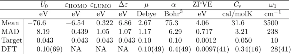
Table 4: Mean and mean absolute deviation (MAD) for all properties in the QM9 data set, as well as target MAE, and DFT (at B3LYP level of theory) MAE relative to experiment for each property, and the number of molecules used to estimate the values (In parentheses of DFT row). The target accuracies taken from Ref.13Target accuracy for energies of atomization, and orbital energies were
set to 1 kcal/mol, which is generally accepted as (or close to) chemical accuracy within the chemistry community. Target accuracies used forµandαare 0.1 D and 0.1 Bohr3 respectively, which is within
the error of CCSD relative to experiments.30 Target accuracies used forω
1 and ZPVE are10cm−1,
which is slightly larger than CCSD(T) error for predicting frequencies.60 Target accuracies used for
Cv were not explained in article.13 Section 2.3 discusses how the errors for DFT where obtained.
U0 εHOMO εLUMO ∆ε µ α ZPVE Cv ω1 eV eV eV eV Debye Bohr3 eV cal/molK cm−1
Mean −76.6 −6.54 0.322 6.86 2.67 75.3 4.06 31.6 3500
MAD 8.19 0.439 1.05 1.07 1.17 6.29 0.717 3.21 238
Target 0.043 0.043 0.043 0.043 0.10 0.10 0.0012 0.050 10
DFT 0.10(69) NA NA NA 0.10(49) 0.4(49) 0.0097(41) 0.34(16) 28(41)
convergence already for relatively small train-ing sets.
RF performs poorly compared to GC, GG and KRR for all properties except for ω1, the
high-est lying fundamental vibrational frequency in each molecule. For this property RF yields an astounding performance with out-of-sample errors as small as single digit cm−1. B3LYP
achieves a mean absolute error of only 28 cm−1
with respect to experiment.32 The distribution
of ω1, Fig. 1 of reference,13 suggests a simple
reason for this: There are three distinct peaks which correspond to typical C-H, N-H and O-H stretch vibrations in increasing order. There-fore the principal learning task in this property is to detect if there is an OH group, and if not if there is an NH group. If neither group is present, CH will yield the vibration with the highest frequency. As such, this is essentially about classifying which bonds are present in the molecule. RF works by fitting a decision tree to the target property. Each branch in the tree is based on an inequality ofoneentry in the
representation. RF should therefore be able to identify which bonds are present in a molecule, simply by looking at the entries in the each el-ement pair, and/or triplet bin of the represen-tations. For RF, a fractional importance can be assigned to each input feature (the sum of all importances is 1.0). Analyzing the impor-tance of the bins in HDAD of the RF model reveals that the three bins with highest
impor-tance are: O-H placed at 0.961 Å, N-H placed at at 1.01 Å and C-C-H at 3.138 radians with
an importance of 0.587, 0.305 and 0.064 respec-tively. These three first bins constitute ∼96%
of the prediction ofω1 and distances of the O-H
and N-H bins are very similar to O-H and N-H bond lengths. C-C-H is placed on ∼π radians
which means that it has to correspond to a lin-ear C-C-H (alkyne) chain which implies that the two carbons must be bonded by a triple bond (typically the C-H with the lowest pKa and the
highest C-H stretch vibration).
KRR performs remarkably well on average. For extensive energetic properties it yields the lowest overall errors in combination with HDAD and BOB, respectively. Its outstand-ing performance is not unsurprisoutstand-ing in light of the multiple previous ML studies dealing with compositional as well as configurational spaces. The neural network flavors GC and GG, how-ever, yield better performance on average, and the lowest errors for all electronic (mostly in-tensive) properties, i.e. dipole moment, polar-izability, HOMO/LUMO eigenvalues and gaps. A possible explanation for this property depen-dent difference in performance between KRR and NN could be the inherent respective addi-tive and multiplicaaddi-tive nature of these regres-sors. The energy being extensive, it is con-sistent with this picture that effective, quasi-particle based linear KRR based estimates have recently been reported to deliver very accurate 11
ACS Paragon Plus Environment
1 2 3 4 5 6 7 8 9 10 11 12 13 14 15 16 17 18 19 20 21 22 23 24 25 26 27 28 29 30 31 32 33 34 35 36 37 38 39 40 41 42 43 44 45 46 47 48 49 50 51 52 53 54 55 56 57 58 59 60
1 2 3 4 5 6 7 8 9 10 11 12 13 14 15 16 17 18 19 20 21 22 23 24 25 26 27 28 29 30 31 32 33 34 35 36 37 38 39 40 41 42 43 44 45 46 47 48 49 50 51 52 53 54 55 56 57 58 59 60
and HD can even yield slightly lower errors than HDAD. In our opinion, this is due to the addi-tional bins of angles and dihedrals rather adding noise than signal. By contrast, the separation of distances, angles and dihedral angles into dif-ferent bins is not a problem for the KRR meth-ods because the kernels used are purely distance based. This makes it possible for KRR to ex-ploit the extra three- and four-body informa-tion in HDAD and to gain an advantage over HD. We note however that the remarkable per-formance of HDAD is possible despite its strik-ing simplicity. As illustrated in Fig. 1 and dis-cussed above, characteristic chemical behavior can be directly obtained by human inspection of HDAD. As such, HDAD corresponds to a rep-resentation very much "Occam’s razor style". Unfortunately, due to its discrete nature and its origin in sorting distances, HDAD will suf-fer from lack of difsuf-ferentiability, which might limit its applicability when modeling forces or other non-equilibrium properties.
MARAD, containing similar information as HDA, performs similarly to BAML—yet, MARAD requires no prior knowledge about the physics encoded in the universal force-field such as electronic hybridization states, bond-order, or functional potential shapes (Morse, Lennard-Jones, harmonic angular potentials, or sinusoidal dihedrals). BOB and CM, previously state of the art, result in relatively poor perfor-mance. ECFP4 produces out-of-sample errors on par or slightly better than CM/KRR for intensive properties (µ, HOMO/LUMO
eigen-values and gap), however the model produces errors that are off-the-chart for all extensive properties (α,ZPVE, U0 and CV).
4
Conclusions
We have benchmarked many combinations of regressors and representations on the same QM9 data set consisting of ∼131k organic molecules. For all properties, the best ML model prediction errors reach the accuracy of DFT at B3LYP level with respect to experi-ment. For 7 out of 12 distinct properties (at-omization energies, heat-capacity, ω1, µ)
out-of-sample errors reach levels on par with chem-ical accuracy, or better, using a training set size of ∼118k (90% of QM9 data set) molecules.
For the remaining properties α, εHOMO,εLUMO, ∆ǫ, and ZPVE, errors of the best models come
within a factor 2 of chemical accuracy.
Regressors EN, BR, and RF lead to rather high out-of-sample errors, while KRR and graph based NN regressors compete for the low-est errors. We have found that GC, GG, and KRR have best performance across all
prop-erties, except for the highest vibrational fre-quency for which RF performs best. There is no single representation and regressor combination that works best for all properties (though forth-coming work with further improvements to the GG based models indicates best in class per-formance across all properties63). For
inten-sive electronic properties (µ, HOMO/LUMO
eigenvalues and gap) we have found MG/NN to yield the highest predictive power, while HDAD/KRR corresponds to the most accurate model for extensive properties (α, ZPVE, U0
and CV). The latter point is remarkable when
considering the simplicity of KRR, being just a linear expansion of property in training set, and HDAD, being just histograms of distances, angles, dihedrals. Using BR and EN is not rec-ommended if accuracy is of importance, both regressors perform worse across all properties. Apart from predicting highest fundamental vi-brational frequency best, RF based models de-liver rather unsatisfactory performance. The ECPF4 based models have shown poor general performance in comparison to all other repre-sentations studied; it is not recommended for investigations of molecular properties.
We should caution the reader that all our re-sults refer to equilibrium structures of a set of only ∼131 k organic molecules. While ∼131k molecules might seem sufficiently large to be representative, this number is dwarfed in com-parison to chemical space, i.e. the space popu-lated by all theoretically stable molecules, es-timated to exceed 1060 for medium sized
or-ganic molecules.64 Furthermore, ML models
for predicting properties of molecules in non-equilibrium or strained configurations might re-quire substantially more training data. This 13
ACS Paragon Plus Environment
1 2 3 4 5 6 7 8 9 10 11 12 13 14 15 16 17 18 19 20 21 22 23 24 25 26 27 28 29 30 31 32 33 34 35 36 37 38 39 40 41 42 43 44 45 46 47 48 49 50 51 52 53 54 55 56 57 58 59 60
point is also of relevance because some of the highly accurate models described herewithin (MG based) currently use bond based graph connectivity in addition to distance, raising questions about the applicability to reactive processes.
In summary, for the organic molecules stud-ied, we have collected numerical evidence which suggests that the out-of-sample error of ML is consistently better than estimated DFT at B3LYP level accuracy. While this is no guar-antee that ML models would reach same error levels if more accurate, explicitly electron corre-lated or experimental reference data was used, previous studies indicate that similar perfor-mance can be expected when using higher levels of theory.8 More specifically, one might
intu-itively expect that going beyond hybrid DFT to higher quality data (either wavefunction based-QM or experiment) in terms of reference meth-ods would represent a more challenging learn-ing problem, and therefore imply the need for larger training set sizes. Results in Ref.,8
how-ever, suggest that ML models can predict the differences between HF and MP2, CCSD, and CCSD(T) equally well using the same training set.
As such, we conclude that future reference datasets for training state-of-the-art machine learning models of molecular properties should preferably use reference levels of theory which go beyond DFT at B3LYP level of accuracy. While it seems unlikely that for each class of molecules, hundreds of thousands of experimen-tal training data points will become available in the foreseeable future, it might well be pos-sible to reach such scale using efficient imple-mentations of explicit electron correlated meth-ods within high-performance computing cam-paigns. Finally, we note that future work could deal with improving representations and regres-sors, with the goal of reaching similar predictive power using less data.
AcknowledgementThe authors thank Dirk
Bakowies for helpful comments, and Adrian Roitberg for pointing out an issue with the use of partial charges in the neural net models in an earlier version of this paper. O.A.v.L.
ac-knowledges support from the Swiss National Science foundation (No. PP00P2_138932, 310030_160067), the research fund of the Uni-versity of Basel, and from Google. This mate-rial is based upon work supported by the Air Force Office of Scientific Research, Air Force Material Command, USAF under Award No. FA9550-15-1-0026. This research was partly supported by the NCCR MARVEL, funded by the Swiss National Science Foundation. Some calculations were performed at sciCORE (http://scicore.unibas.ch/) scientific comput-ing core facility at University of Basel.
5
SI
Supplementary information regarding raw data, MARAD representation, graph convolutions, gated graphs, random forests, and learning curves are reported, as well as root mean square errors for ML predictions after training on the largest training set.
1 2 3 4 5 6 7 8 9 10 11 12 13 14 15 16 17 18 19 20 21 22 23 24 25 26 27 28 29 30 31 32 33 34 35 36 37 38 39 40 41 42 43 44 45 46 47 48 49 50 51 52 53 54 55 56 57 58 59 60
References
(1) Hohenberg, P.; Kohn, W. Inhomogeneous Electron Gas.Phys. Rev.1964,136, B864.
(2) Kohn, W.; Sham, L. J. Self-Consistent Equations Including Exchange and Cor-relation Effects. Phys. Rev. 1965, 140,
A1133.
(3) Burke, K. Perspective on density func-tional theory. J. Chem. Phys. 2012, 136,
150901.
(4) Koch, W.; Holthausen, M. C.A Chemist’s Guide to Density Functional Theory;
Wiley-VCH, 2002.
(5) Cohen, A. J.; Mori-Sánchez, P.; Yang, W. Challenges for Density Functional Theory.
Chem. Rev. 2012, 112, 289–320.
(6) Plata, R. E.; Singleton, D. A. A Case Study of the Mechanism of Alcohol-Mediated Morita Baylis-Hillman Reac-tions. The Importance of Experimental Observations. J. Am. Chem. Soc. 2015,
137, 3811–3826.
(7) Medvedev, M. G.; Bushmarinov, I. S.; Sun, J.; Perdew, J. P.; Lyssenko, K. A. Density functional theory is straying from the path toward the exact functional. Sci-ence 2017,355, 49–52.
(8) Ramakrishnan, R.; Dral, P. O.; Rupp, M.; von Lilienfeld, O. A. Big Data Meets Quantum Chemistry Approximations: The ∆-Machine Learning Approach. J. Chem. Theory Comput. 2015, 11,
2087–2096.
(9) Ramakrishnan, R.; Dral, P. O.; Rupp, M.; von Lilienfeld, O. A. Quantum chem-istry structures and properties of 134 kilo molecules. Sci. Data 2014,1, 140022.
(10) Ruddigkeit, L.; van Deursen, R.; Blum, L. C.; Reymond, J.-L. Enu-meration of 166 Billion Organic Small Molecules in the Chemical Universe Database GDB-17. J. Chem. Inf. Model.
2012, 52, 2864–2875.
(11) Huang, B.; von Lilienfeld, O. A. Commu-nication: Understanding molecular repre-sentations in machine learning: The role of uniqueness and target similarity.J. Chem. Phys 2016, 145, 161102.
(12) Hansen, K.; Biegler, F.; Ramakrish-nan, R.; Pronobis, W.; von Lilien-feld, O. A.; Müller, K.-R.; Tkatchenko, A. Machine Learning Predictions of Molec-ular Properties: Accurate Many-Body Potentials and Nonlocality in Chemical Space. J. Phys. Chem. Lett. 2015, 6,
2326–2331.
(13) Ramakrishnan, R.; von Lilienfeld, O. A. Many Molecular Properties from One Ker-nel in Chemical Space. chimia 2015, 69,
182–186.
(14) Rupp, M.; Tkatchenko, K.-R., Alexandre haand Müller; von Lilienfeld, O. A. Fast and Accurate Modeling of Molecular At-omization Energies with Machine Learn-ing. Phys. Rev. Lett. 2012,108, 058301.
(15) Barker, J.; Bulin, J.; Hamaekers, J.; Mathias, S. Localized Coulomb Descrip-tors for the Gaussian Approximation Po-tential. arXiv preprint arXiv:1611.05126
2016,
(16) von Lilienfeld, O. A.; Ramakrishnan, R.; Rupp, M.; Knoll, A. Fourier series of atomic radial distribution functions: A molecular fingerprint for machine learning models of quantum chemical properties.
Int. J. Quantum 2015, 115, 1084–1093. (17) Huan, T. D.; Mannodi-Kanakkithodi, A.;
Ramprasad, R. Accelerated materials property predictions and design using motif-based fingerprints. Phys. Rev. B
2015,92, 014106.
(18) Bartók, A. P.; Kondor, R.; Csányi, G. On representing chemical environments.Phys. Rev. B 2013, 87, 184115.
(19) De, S.; Bartók, A. P.; Csányi, G.; Ceri-otti, M. Comparing molecules and solids across structural and alchemical space. 15
ACS Paragon Plus Environment
1 2 3 4 5 6 7 8 9 10 11 12 13 14 15 16 17 18 19 20 21 22 23 24 25 26 27 28 29 30 31 32 33 34 35 36 37 38 39 40 41 42 43 44 45 46 47 48 49 50 51 52 53 54 55 56 57 58 59 60
Phys. Chem. Chem. Phys. 2016, 18, 13754–13769.
(20) Collins, C. R.; Gordon, G. J.; von Lilienfeld, O. A.; Yaron, D. J. Con-stant Size Molecular Descriptors For Use With Machine Learning. arXiv preprint arXiv:1701.06649 2016,
(21) Smith, J. S.; Isayev, O.; Roitberg, A. E. ANI-1: An extensible neural network po-tential with DFT accuracy at force field computational cost. Chem. Sci. 2017, 8,
3192–3203.
(22) Schütt, K. T.; Arbabzadah, F.; Chmiela, S.; Müller, K. R.; Tkatchenko, A. Quantum-chemical in-sights from deep tensor neural networks.
Nat. Commun. 2017,8, 13890.
(23) Dral, P. O.; von Lilienfeld, O. A.; Thiel, W. Machine Learning of Parame-ters for Accurate Semiempirical Quantum Chemical Calculations. J. Chem. Theory
2015, 11, 2120–2125.
(24) Weber, W.; Thiel, W. Orthogonaliza-tion correcOrthogonaliza-tions for semiempirical meth-ods. Theor. Chem. Acc. 2000, 103, 495–
506.
(25) Dral, P. O.; Wu, X.; Spörkel, L.; Koslowski, A.; Thiel, W. Semiempirical Quantum-Chemical Orthogonalization-Corrected Methods: Benchmarks for Ground-State Properties. J. Chem. Theory 2016, 12, 1097–1120.
(26) Hansen, K.; Montavon, G.; Biegler, F.; Fa-zli, S.; Rupp, M.; Scheffler, M.; von Lilien-feld, O. A.; Tkatchenko, A.; Müller, K.-R. Assessment and Validation of Machine Learning Methods for Predicting Molecu-lar Atomization Energies. J. Chem. The-ory Comput.2013, 9, 3404–3419.
(27) Kearnes, S.; McCloskey, K.; Berndl, M.; Pande, V.; Riley, P. Molecular Graph Con-volutions: Moving Beyond Fingerprints.
J. Comput. Aided Mol. Des. 2016, 30, 595–608.
(28) Li, Y.; Tarlow, D.; Brockschmidt, M.; Zemel, R. Gated Graph Sequence Neural Networks. ICLR 2016,
(29) Curtiss, L. A.; Raghavachari, K.; Red-fern, P. C.; Pople, J. A. Assessment of Gaussian-2 and density functional theories for the computation of enthalpies of for-mation.J. Chem. Phys. 1997, 106, 1063–
1079.
(30) Hickey, A. L.; Rowley, C. N. Benchmark-ing quantum chemical methods for the cal-culation of molecular dipole moments and polarizabilities. J. Phys. Chem. A 2014,
118, 3678–3687.
(31) Stowasser, R.; Hoffmann, R. What do the Kohn-Sham orbitals and eigenvalues mean? J. Am. Chem. Soc. 1999, 121, 3414.
(32) Sinha, P.; Boesch, S. E.; Gu, C.; Wheeler, R. A.; Wilson, A. K. Harmonic Vibrational Frequencies: Scaling Factors for HF, B3LYP, and MP2 Methods in Combination with Correlation Consistent Basis Sets. J. Phys. Chem. A 2004, 108,
9213–9217.
(33) Geary, R. C. The Ratio of the Mean Devi-ation to the Standard DeviDevi-ation as a Test of Normality. Biometrika 1935, 27, 310–
332.
(34) DeTar, D. F. Calculation of Entropy and Heat Capacity of Organic Compounds in the Gas Phase. Evaluation of a Consistent Method without Adjustable Parameters. Applications to Hydrocarbons. J. Phys. Chem. A 2007, 111, 4464–4477.
(35) Huo, H.; Rupp, M. Unified Representation for Machine Learning of Molecules and Crystals.arXiv preprint arXiv:1704.06439
2017,
(36) Bartok, A. P.; De, S.; Poelking, C.; Bern-stein, N.; Kermode, J.; Csanyi, G.; Ce-riotti, M. Machine Learning Unifies the Modelling of Materials and Molecules.
arXiv preprint arXiv:1706.00179 2017,
1 2 3 4 5 6 7 8 9 10 11 12 13 14 15 16 17 18 19 20 21 22 23 24 25 26 27 28 29 30 31 32 33 34 35 36 37 38 39 40 41 42 43 44 45 46 47 48 49 50 51 52 53 54 55 56 57 58 59 60
(37) Rappe, A. K.; Casewit, C. J.; Col-well, K. S.; III, W. A. G.; Skiff, W. M. UFF, a full periodic table force field for molecular mechanics and molecular dy-namics simulations. J. Am. Chem. Soc.
1992, 114, 10024–10035.
(38) Rogers, D.; Hahn, M. Extended-connectivity fingerprints. J. Chem. Inf. Model. 2010,50, 742–754.
(39) Besnard, J.; Ruda, G. F.; Setola, V.; Abecassis, K.; Rodriguiz, R. M.; Huang, X.-P.; Norval, S.; Sassano, M. F.; Shin, A. I.; Webster, L. A.; Sime-ons, F. R. C.; Stojanovski, L.; Prat, A.; Seidah, N. G.; Constam, D. B.; Bicker-ton, G. R.; Read, K. D.; Wetsel, W. C.; Gilbert, I. H.; Roth, B. L.; Hopkins, A. L. Automated design of ligands to polyphar-macological profiles. Nature 2012, 492,
215–220.
(40) Lounkine, E.; Keiser, M. J.; White-bread, S.; Mikhailov, D.; Hamon, J.; Jenkins, J. L.; Lavan, P.; Weber, E.; Doak, A. K.; Côté, S.; Shoichet, B. K.; Urban, L. Large-scale prediction and test-ing of drug activity on side-effect targets.
Nature 2012, 486, 361–367.
(41) Huigens III, R. W.; Morrison, K. C.; Hick-lin, R. W.; Flood Jr, T. A.; Richter, M. F.; Hergenrother, P. J. A Ring Distortion Strategy to Construct Stereochemically Complex and Structurally Diverse Com-pounds from Natural Products. Nature chemistry 2013,5, 195.
(42) Todeschini, R.; Consonni, V. Handbook of Molecular Descriptors; Wiley-VCH,
Weinheim, 2009.
(43) Faulon, J.-L.; Visco, Jr., D. P.; Pophale, R. S. The Signature Molec-ular Descriptor. 1. Using Extended Valence Sequences in QSAR and QSPR Studies. J. Chem. Inf. Comp. Sci. 2003,
43, 707.
(44) Visco, J.; Pophale, R. S.; Rintoul, M. D.; Faulon, J. L. Developing a methodology
for an inverse quantitative structure activ-ity relationship using the signature molec-ular descriptor. J. Mol. Graph. Model.
2002,20, 429–438.
(45) O’Boyle, N. M.; Banck, M.; James, C. A.; Morley, C.; Vandermeersch, T.; Hutchi-son, G. R. Open Babel: An open chemical toolbox. J. Cheminform. 2011, 3, 1–14.
(46) Landrum, G. RDKit: Open-source chem-informatics. http://www.rdkit.org 2014,
3, 2012.
(47) Faber, F. A.; Hutchison, L.; Huang, B.; Gilmer, J.; Schoenholz, S. S.; Dahl, G. E.; Vinyals, O.; Kearnes, S.; Riley, P. F.; von Lilienfeld, O. A. Fast machine learning models of electronic and energetic propties consistently reach approximation er-rors better than DFT accuracy. arXiv preprint arXiv:1702.05532 2017,
(48) Müller, K.-R.; Mika, S.; Rätsch, G.; Tsuda, K.; Schölkopf, B. An introduction to kernel-based learning algorithms.IEEE transactions on neural networks 2001,12,
181–201.
(49) Schölkopf, B.; Smola, A. J. Learning with kernels: support vector machines, regular-ization, optimregular-ization, and beyond; MIT
press, 2002.
(50) Vovk, V. In Empirical Inference: Festschrift in Honor of Vladimir N. Vapnik; Schölkopf, B., Luo, Z., Vovk, V.,
Eds.; Springer Berlin Heidelberg: Berlin, Heidelberg, 2013; pp 105–116.
(51) Hastie, T.; Tibshirani, R.; Friedman, J.
The Elements of Statistical Learning: Data Mining, Inference, and Prediction, Second Edition, 2nd ed.; Springer: New
York, 2011.
(52) Hoerl,; Arthur, E.; Kennard,; Robert, W. Ridge Regression Biased Estimation for Nonorthogonal Problems. Technometrics
2000, 80.
17
ACS Paragon Plus Environment
1 2 3 4 5 6 7 8 9 10 11 12 13 14 15 16 17 18 19 20 21 22 23 24 25 26 27 28 29 30 31 32 33 34 35 36 37 38 39 40 41 42 43 44 45 46 47 48 49 50 51 52 53 54 55 56 57 58 59 60
(53) Pedregosa, F.; Varoquaux, G.; Gram-fort, A.; Michel, V.; Thirion, B.; Grisel, O.; Blondel, M.; Prettenhofer, P.; Weiss, R.; Dubourg, V.; Vanderplas, J.; Passos, A.; Cournapeau, D.; Brucher, M.; Perrot, M.; Duchesnay, E. Scikit-learn: Machine Learning in Python. J. Mach. Learn. Res. 2011, 12, 2825–2830.
(54) Neal, R. M. Bayesian Learning for Neu-ral Networks; Springer-Verlag New York, Inc.: Secaucus, NJ, USA, 1996.
(55) Zou, H.; Hastie, T. Regularization and variable selection via the elastic net.J. R. Stat. Soc. Series. B Stat. Methodol. 2005,
67, 301–320.
(56) Breiman, L. Random forests. Machine learning 2001, 45, 5–32.
(57) Duvenaud, D. K.; Maclaurin, D.; Ipar-raguirre, J.; Bombarell, R.; Hirzel, T.; Aspuru-Guzik, A.; Adams, R. P. Convo-lutional Networks on Graphs for Learning Molecular Fingerprints. Advances in Neu-ral Information Processing Systems. 2015; pp 2215–2223.
(58) Desautels, T.; Krause, A.; Burdick, J. W. Parallelizing Exploration-Exploitation Tradeoffs in Gaussian Process Bandit Optimization.J. Mach. Learn. Res.2014,
15, 4053–4103.
(59) Google HyperTune. https://cloud.google.com/ml/ (accessed 2016).
(60) Tew, D. P.; Klopper, W.; Heckert, M.; Gauss, J. Basis Set Limit CCSD(T) Har-monic Vibrational Frequencies. J. Phys. Chem. A 2007, 111, 11242–11248.
(61) Müller, K.-R.; Finke, M.; Murata, N.; Schulten, K.; Amari, S. A numerical study on learning curves in stochastic multi-layer feedforward networks. Neural Com-put.1996, 8, 1085–1106.
(62) Huang, B.; von Lilienfeld, O. A. The “DNA” of chemistry: Scalable quantum
machine learning with “amons”. arXiv preprint arXiv:1707.04146 2017,
(63) Gilmer, J.; Schoenholz, S. S.; Riley, P. F.; Vinyals, O.; Dahl, G. E. Neural Message Passing for Quantum Chemistry. Proceed-ings of the 34nd International Conference on Machine Learning, ICML 2017. 2017. (64) Kirkpatrick, P.; Ellis, C. Chemical space.
Nature 2004,432, 823. 1 2 3 4 5 6 7 8 9 10 11 12 13 14 15 16 17 18 19 20 21 22 23 24 25 26 27 28 29 30 31 32 33 34 35 36 37 38 39 40 41 42 43 44 45 46 47 48 49 50 51 52 53 54 55 56 57 58 59 60
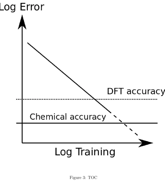
Figure 3: TOC
19
ACS Paragon Plus Environment
1 2 3 4 5 6 7 8 9 10 11 12 13 14 15 16 17 18 19 20 21 22 23 24 25 26 27 28 29 30 31 32 33 34 35 36 37 38 39 40 41 42 43 44 45 46 47 48 49 50 51 52 53 54 55 56 57 58 59 60