Experimentation
by
Guy Emerton
Thesis presented in partial fullment of the requirements for
the degree of Master of Sciences in the Institute for Wine
Biotechnology, Faculty of AgriSciences at Stellenbosch
University
Institute of Wine Biotechnology, University of Stellenbosch,
Private Bag X1, Matieland 7602, South Africa.
Supervisor: Dr. Daniel Jacobson
Declaration
By submitting this thesis electronically, I declare that the entirety of the work contained therein is my own, original work, that I am the sole author thereof (save to the extent explicitly otherwise stated), that reproduction and pub-lication thereof by Stellenbosch University will not infringe any third party rights and that I have not previously in its entirety or in part submitted it for obtaining any qualication.
Signature: . . . . G. Emerton
2013/12/20
Date: . . . .
Copyright © 2014 Stellenbosch University All rights reserved.
We often forget how science and engineering function. Ideas come from previous exploration more often than from lightning strokes. Important ques-tions can demand the most careful planning for conrmatory analysis. Broad general inquiries are also important. Finding the questions is often more im-portant than nding the answer. Exploratory data analysis is an attitude, a exibility, and a reliance on display, NOT a bundle of techniques, and should so be taught. Conrmatory data anlaysis, by contrast, is easier to teach and easer to computerize. We need to teach both; to think about science and engi-neering more broadly; to be prepared to randomize and avoid multiplicity. John W. Tukey, 1980
Abstract
Data-Driven Methods for Exploratory Analysis in
Chemometrics and Scientic Experimentation
G. Emerton
Institute of Wine Biotechnology, University of Stellenbosch,
Private Bag X1, Matieland 7602, South Africa.
Thesis: Master of Science in Wine Biotechnology March 2014
Background
New methods to facilitate exploratory analysis in scientic data are in high demand. There is an abundance of available data used only for conrmatory analysis from which new hypotheses can be drawn. To this end, two new exploratory techniques are developed: one for chemometrics and another for visualisation of fundamental scientic experiments. The former transforms large-scale multiple raw HPLC/UV-vis data into a conserved set of putative features - something not often attempted outside of Mass-Spectrometry. The latter method ('StatNet'), applies network techniques to the results of designed experiments to gain new perspective on variable relations.
Results
The resultant data format from un-targeted chemometric processing was amenable to both chemical and statistical analysis. It proved to have in-tegrity when machine-learning techniques were applied to infer attributes of the experimental set-up. The visualisation techniques were equally successful in generating hypotheses, and were easily extendible to three dierent types of experimental results.
Conclusion
The overall aim was to create useful tools for hypothesis generation in a variety of data. This has been largely reached through a combination of novel and existing techniques. It is hoped that the methods here presented are further applied and developed.
Uittreksel
Data-Driven Methods for Exploratory Analysis in
Chemometrics and Scientic Experimentation
G. Emerton
Institute of Wine Biotechnology, University of Stellenbosch,
Private Bag X1, Matieland 7602, South Africa.
Thesis: Magister in die Natuurwetenskappe in Wyn Biotegnologie March 2014
Agtergrond
Nuwe metodes om ondersoekende ontleding in wetenskaplike data te fasili-teer is in groot aanvraag. Daar is 'n oorvloed van beskikbaar data wat slegs gebruik word vir bevestigende ontleding waaruit nuwe hipoteses opgestel kan word. Vir hierdie doel, word twee nuwe ondersoekende tegnieke ontwikkel: een vir chemometrie en 'n ander vir die visualisering van fundamentele wetenskap-like eksperimente. Die eersgenoemde transformeer grootskaalse veelvoudige rou HPLC / UV-vis data in 'n bewaarde stel putatiewe funksies - iets wat nie gereeld buite Massaspektrometrie aangepak word nie. Die laasgenoemde metode ('StatNet') pas netwerktegnieke tot die resultate van ontwerpte eksper-imente toe om sodoende ân nuwe perspektief op veranderlike verhoudings te verkry.
Resultate
Die gevolglike data formaat van die ongeteikende chemometriese verwerking was in 'n formaat wat vatbaar is vir beide chemiese en statistiese analise. Daar is bewys dat dit integriteit gehad het wanneer masjienleertegnieke toegepas is om eienskappe van die eksperimentele opstelling af te lei. Die visualiser-ingtegnieke was ewe suksesvol in die generering van hipoteses, en ook maklik uitbreibaar na drie verskillende tipes eksperimentele resultate.
Samevatting
Die hoofdoel was om nuttige middele vir hipotese generasie in 'n verskei-denheid van data te skep. Dit is grootliks bereik deur 'n kombinasie van oor-spronklike en bestaande tegnieke. Hopelik sal die metodes wat hier aangebied is verder toegepas en ontwikkel word.
Acknowledgements
I would like to express my sincere gratitude to the following people and organ-isations: my supervisor Daniel Jacobson for direction, guidance and tutelage; as well as the Institute for Wine Biotechnology (IWBT) for facilitating this study and providing such excellent opportunities for the application of these developed techniques. Within the institute, thanks must go to the Computa-tional Biology research group as a whole for advice and assistance, especially Piet Jones who gave tireless advice on statistics and parallelisation. Further acknowledgments are due to Phillip Rosochacki for his enthusiastic assistance with machine learning techniques; Adriaan Haasbroek for excellent morale boosting and my family for their unconditional support. Also to Danie Coet-see for his help in translation.
Special thanks to Dr. Astrid Buica, whose excellent data collection from a very large-scale experiment was the basis for much of this thesis; also to her advice on the development of StatNet which was invaluable. My gratitude is also extended to Carien Coetzee for collaboration on the visualisation of her sensory experiment, as well as Kari du Plessis who made her data available for testing.
Contents
Declaration i Acknowledgements v Contents vi List of Figures ix 1 Introduction 1 1.1 Background . . . 1 1.1.1 Chemometrics . . . 11.1.2 Network Visualisation - StatNet . . . 2
1.2 Problem Statement . . . 2 1.3 Aims . . . 3 1.4 Chapter Overview . . . 3 2 Literature Review 4 2.1 Chemometric Literature . . . 4 2.1.1 Experimental Data . . . 4 2.1.2 Chemometric Methods . . . 5 2.1.2.1 Wavelets . . . 5
2.1.2.2 Savitzky-Golay Smoothing Filter . . . 7
2.1.2.3 Baseline Correction . . . 8
2.1.2.4 2-Dimensional Alignment . . . 9
2.1.2.4.1 Methods Review . . . 9
2.1.2.4.2 AlignDE . . . 10
2.1.2.4.3 COW . . . 11
2.1.2.5 Feature Map Alignment . . . 13
2.1.3 Machine Learning Techniques . . . 15
2.1.3.1 Decision Trees . . . 16
2.1.3.2 Principal Component Analysis . . . 17
2.1.3.3 Network Analysis . . . 17
2.2 StatNet Literature . . . 18
2.2.1 Background . . . 18 vi
2.2.2 Network Visualisation . . . 19
2.2.3 Temporal Data . . . 20
2.2.4 Principal Component Analysis . . . 21
2.2.5 Data Interaction . . . 21
2.2.6 Statistical Methods . . . 22
2.2.6.1 Metrics . . . 22
2.2.6.2 Statistical Tests . . . 22
2.2.6.3 Correction for Multiple Hypothesis Testing . . . 23
2.3 Conclusion . . . 24 2.4 List of References . . . 26 3 Chemometric Analysis 30 3.1 Introduction . . . 30 3.1.1 HPLC/UV-vis . . . 30 3.1.2 Technical Issues . . . 31 3.1.3 Data . . . 31 3.1.4 Purpose . . . 32 3.2 Methodology . . . 32 3.2.1 Preprocessing . . . 33 3.2.1.1 Data Parsing . . . 33
3.2.1.2 Baseline Correction and Smoothing . . . 34
3.2.1.3 Alignment . . . 34
3.2.1.4 Peak Detection . . . 39
3.2.2 Feature Matrix Generation . . . 44
3.2.2.1 Problem Statement . . . 44
3.2.2.2 Overview . . . 45
3.2.2.3 Aggregating Peak Features . . . 46
3.2.2.4 Experiment-Database Alignment . . . 49
3.3 Results and Discussion . . . 52
3.3.1 PCA . . . 52
3.3.2 Decision Trees . . . 57
3.3.3 Chemical Network . . . 65
3.3.3.1 Network Layout . . . 65
3.3.3.2 Maximum Spanning Tree . . . 66
3.3.3.3 Correlation Network . . . 66
3.3.3.4 Focused Correlation Network . . . 66
3.4 Conclusion . . . 71 3.5 Acknowlegments . . . 72 3.6 List of References . . . 73 4 Network Visualisation 76 4.1 Introduction . . . 76 4.2 Methodology . . . 77 4.2.1 Experimental Data . . . 77
4.2.2 Network creation . . . 78
4.3 Results and Discussion . . . 79
4.3.1 Sensory Data . . . 79
4.3.1.1 Correlation Network . . . 79
4.3.1.2 Central Composite Network . . . 80
4.3.2 Botrytis Infection . . . 82 4.3.2.1 All-against-all Network . . . 82 4.3.2.2 ET50 Network . . . 84 4.3.2.3 Time-centric Network . . . 84 4.3.3 Browning Experiment . . . 84 4.3.3.1 Time-centric Network . . . 87
4.3.3.2 Tiered Variable Network . . . 87
4.3.3.3 Star Network . . . 89 4.4 Conclusion . . . 91 4.5 Acknowledgments . . . 91 4.6 List of References . . . 91 5 Conclusion 93 5.1 Summary . . . 93 5.2 Conclusion . . . 93 5.3 Future Perspectives . . . 94
List of Figures
2.1 Mexican Hat Wavelet . . . 6
2.2 Savitzky-Golay Noise Filter . . . 7
2.3 Warping Optimisation . . . 12
2.4 Time Wheel Visualisation . . . 21
3.1 Baseline correction of Chromatograms . . . 35
3.2 Wavelength-wise Alignment . . . 37
3.3 TAC Alignment . . . 39
3.4 Continuous Wavelet Transform for Peak Detection . . . 40
3.5 SNR ratios . . . 41
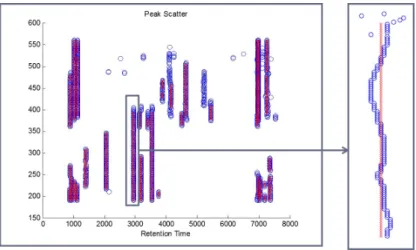
3.6 Final Peak Plot . . . 41
3.7 Peak Detection at High Wavelength . . . 42
3.8 Minimum Noise Level Thresholding . . . 43
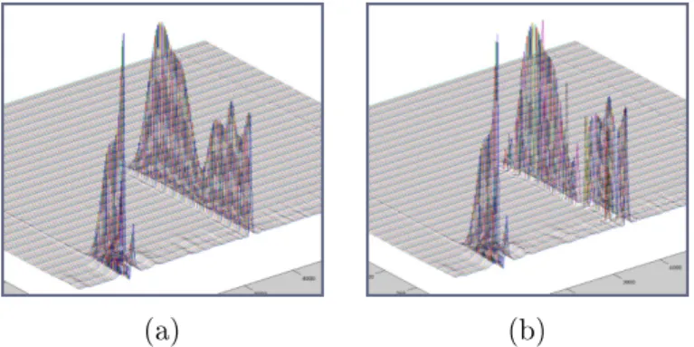
3.9 Peak Landscape Plots . . . 43
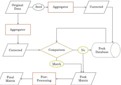
3.10 Peak Comparison Workow . . . 46
3.11 Peak Detection Drift . . . 47
3.12 Peak Aggregation . . . 49
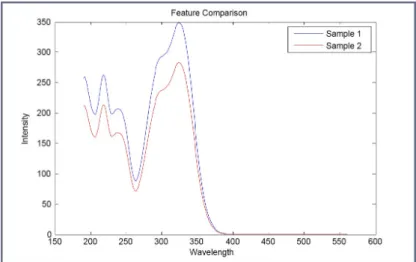
3.13 Feature Comparison . . . 50
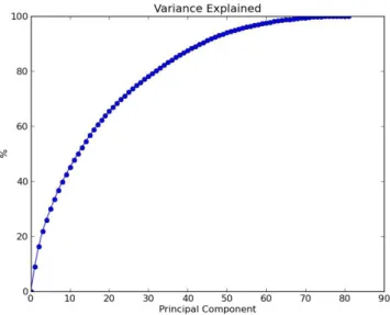
3.14 Variance explained by PCA on entire feature matrix . . . 53
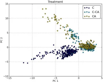
3.15 Score plot of treatment - 2D . . . 54
3.16 Score plot of treatment - 3D, no normalisation . . . 55
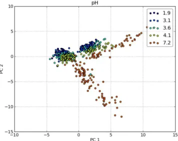
3.17 Score plot with labelled pH levels . . . 55
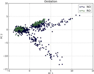
3.18 Score plot with labelled oxidation type . . . 56
3.19 Score plot of time with a reduced data set . . . 57
3.20 Loading plot of PCA on entire data set . . . 58
3.21 Loading plot of PCA on reduced data set . . . 59
3.22 Decision tree for treatment class . . . 60
3.23 Gini importance for variables in the decision tree for treatment . . . 60
3.24 Decision tree for pH class . . . 61
3.25 Gini importance for variables in the decision tree for ph . . . 61
3.26 Decision tree for oxidation class . . . 63
3.27 Gini importance for variables in the decision tree for oxidation . . . 64
3.28 Random permutation tests on decision tree models for each exper-imental condition . . . 64
3.29 Maximum spanning tree derived from full feature matrix . . . 67
3.30 Correlation network with threshold of 0.5, derived from full feature matrix . . . 68
3.31 Correlation network with threshold of 0.5, derived from a single experiment . . . 69
3.32 Maximum spanning tree of single experiment . . . 70
3.33 Comparison of negatively correlated features in a single experiment 70 4.1 Correlation network for orthogonal sensory data . . . 80
4.2 Overall sensory network for central composite experiment . . . 81
4.3 Focused sensory interaction network . . . 83
4.4 PCA loadings of sensory experiment . . . 83
4.5 All-againt-all comparison of infection rate . . . 85
4.6 ET50 of infection rate . . . 86
4.7 Subgraph of strain infection at one time point . . . 86
4.8 Overview of time network for browning data . . . 88
4.9 Focused view of time network for browning data . . . 88
4.10 Tiered network centered on treatment . . . 89
4.11 Complete 'star' network for browning data . . . 90
Chapter 1
Introduction
Modern developments in computation and technology have allowed for biology to become a data rich science. Advances in the ability to derive information from, for example, genetic and chemical samples have caused a deluge in the available data for analysis; such that it is necessary to continually develop new methods for handling and interpreting this inux of information.
This provides platforms for both the generation of new types of data, as well as novel insights into pre-existing data. In this study, focus is lent to the latter, whereby methods are developed to mine data for information which would otherwise be overlooked. The focus is not in the experiments themselves - how the data is generated and collected - but on methods of interpretation after the fact.
To this end, methods for two dierent purposes are covered: rstly, the processing and interpretation of chemometric data; secondly, the interpretation of the results of various experiments, using network analyses.
1.1 Background
1.1.1 Chemometrics
Chemometrics is the application of data-driven methods to chemical data in order to deconvolute the high-dimensional outputs of common analytical chem-istry tools. It augments the trained chemist's ability to manually search and quantify target chemicals from an analysis by rstly, correcting for technical error from the machine; and secondly, oering an analysis of the resultant data in such a way as to deliver results that would otherwise not be realised by inspection.
The untargeted approach in chemometrics is a "bottom-up" approach whereby putative molecules that inuence the data in interesting ways can later be identied. This is in contrast to the traditional analysis method of
ing compounds of interest before the chemical analysis, then tracking their quantitative change exclusively across experimental perturbations.
Methods are here developed to allow for this type of untargeted analysis in large-scale experiments. Within these experiments, variables and condi-tions are perturbed to dierent degrees so that compounds are not necessarily conserved across all measurements - causing chemical heterogeneity between samples. Additionally, the samples were taken over a time series, adding a fur-ther layer of complexity. This massive and multi-modal data set necessitated a relatively novel development and combination of analysis tools in order to compare chemical phenomena across samples.
1.1.2 Network Visualisation - StatNet
Networks are excellent tools for visualisation of complex relationships within data. One such kind of complex data is that which is typically generated from scientic experimentation - the targeted perturbation of input variables in order to gauge the level of some output. The visualisation of these kinds of scientic data is still largely facilitated by classical methods of line, scatter and box plots.
It is contended that networks can be used as an alternative for visualising the results from scientic experiments, not only to draw conclusions from the original hypotheses behind the experiment, but to generate new hypotheses as well. Not only are they amenable to interpretation by the human mind, they also lend themselves to advanced user interaction. In this way networks can represent trends on a large scope, as well as execute advanced queries through ltering, nearest-neighbor searches and subgraph generation. To this end a set of related methods are devised, dubbed 'StatNet'.
Several data sets generated by scientic experimentation are subjected to this network analyses in order to assess their viability. Although they are all related to the eld of wine biotechnology and chemistry, as data types and structures they dier widely. Dierent variations of similar network workows are applied to each, with the central theme being the statistical testing for signicant results followed by structured representation.
1.2 Problem Statement
The traditional scientic method prescribes a cycle of hypothesis and con-rmation. While this is useful for targeted investigation of phenomena, the generation of new hypotheses is often overlooked. This is notable in chemomet-ric analysis, where the vast majority of analyses on data is targeted on specic molecules with conjectured concentrations in the substance in question. This approach is also present to a lesser extent in general scientic investigation with experimental setups targeted towards the answer of a preconceived
prob-lem. In this case the traditional visualisations of results can be overwhelming and often confound the search for new hypotheses.
1.3 Aims
The primary and overarching aim is to develop novel methods for exploratory analysis and hypothesis generation. This common aim is pursued along two dierent avenues: rstly, a large scale generation of putative features from raw machine-generated data; secondly, innovative visualisation of small scale data collected through targeted scientic experimentation.
Aims specically related to chemometrics are to develop a workow both simple and ecient enough to process the chromatograms of a large and ex-haustive experiment, and ultimately to detect putative compounds and derive experimental conclusions about them. Thereafter, to coerce the data into a format amenable to statistical and machine-learning exploration; specically, some representation of putative features. As the chemometric data is derived from a targeted experiment, validation of the original hypotheses through such exploration forms a further aim.
Regarding the second channel of data exploration, the aim is to build on research into generalised and extensible methods of network visualisation (ten-tatively named 'StatNet') that can be broadly applied. The nal product should be something that is intuitive to explore; able to present answers to the original hypothesis, and have the latent facility to generate new ones.
1.4 Chapter Overview
The thesis is split into ve chapters. Following the present chapter, there is a single literature review chapter covering all of the pertinent literature for both the research chapters. The research chapters are split in two: the rst (Chapter 3) will cover the body of chemometric work and includes a discrete introduction, results and conclusion. The second (Chapter 4), contains the majority of the research for network visualisation with a similar structure. The nal chapter contains a nal conclusion to the overall thesis.
Chapter 2
Literature Review
2.1 Chemometric Literature
2.1.1 Experimental Data
An interesting model case for a large-scale experiment with HPLC/UV-vis data is that of Buica (2012) into the eects and causes of browning in white wine during aging. Several conditions were directly altered in order to observe their combined eect on browning and oxygen levels in model wine. One of the main sources of variance was the addition two phenolic compounds in three separate treatments.
Phenols constitute some of the most important compounds in wine, con-tributing to the aroma, colour and palette. In their study into the brown-ing of white wine, Kallithraka et al. (2009) observed the changes in phenolic compounds over time as well as their correlation to various browning mea-sures. Two of the most signicant phenolic compounds were Caeic Acid and Catechin - cited as two phenolic compounds inuencing browning, leading to the formation of by-products due to polymerisation of ortho-quinones (Guyot et al., 1996). The uctuations of these phenols also aects the avour prole of the wine. Kallithraka et al. (2009) found that the concentration of Catechin decreased over time in the experiment; whereas Caeic Acid was one of the few phenols that increased during aging.
A further eect that was studied was the addition of sulphur dioxide. This has the ability to reduce the same ortho-quinones created by the presence of Caeic Acid and Catechin (Singleton, 1987). Simpson (1982), however, found that the inhibitory eects of SO2 were eeting; ineective in the advanced
stages of browning once depleted.
In a large study regarding the overall kinetic eects of aging in white wine, Ferreira (2002) found that the majority of chemical uctuations occurring during the aging process were a result of the eects of oxidation, and pH-induced reactions - in that order. These two are linked by the fact that phenols can suer autoxidation, which leads to rapid consumption of oxygen within the
media. Autoxidation of phenols is extremely sensitive to pH level, as conrmed by Ferreira (2002) in the same work; a dierence of 3- or 4 pH was noted to have the capacity to alter the rate of autoxidation up to 9 times for certain compounds.
2.1.2 Chemometric Methods
In a eld such as chemometrics, in which there has been a long and vested data analytic interest, there are a wealth of techniques that allow for the analysis of extremely complex data types. The particular type of data commonly sub-jected to such analyses is High-Performance Liquid Chromatography (HPLC) with UV/vis spectra. This is a chromatographic technique coupled with ab-sorbance spectrometry, which produces a continuous abab-sorbance feature for each time point. Currently it is common (especially with metabolomics) to couple chromatography with mass spectrometry. This produces a discrete set of mass/charge ratios for each feature; in contrast to the continuous nature of absorbance spectroscopy, with the result that many of the algorithms and software developed are not compatible across these two dierent types of de-tectors.
The individual methods used for parts of the overall analysis are reviewed in sections 2.1.2.1 to 2.1.2.4 below. A review of some of the pertinent software and algorithms for the feature map alignment problem for mass spectroscopic analysis is given in section 2.1.2.5 for comparison to the custom feature align-ment method presented in the next chapter.
2.1.2.1 Wavelets
Many of the contemporary methods used in chemometric analysis are make use of wavelet transforms in some manner. In particular, the baseline correction and peak detection implementations often used are based on these transforms. This type of analysis is gaining increased popularity due to the arrival of computational capacity allowing for it's somewhat intensive execution.
Throughout much of the history of chemometrics, Fourier analysis was the dominant peak deconvolution approach. Fourier theorems propound the hypothesis that any signal can be reduced to a series of sines and cosines in what is known as Fourier expansion. A problem with Fourier expansion is that it describes a signal in frequency space, but loses the measure of time due to Heisenberg's uncertainty principle. In signal processing terms this is expressed by the fact that it is not possible to know both the frequency and the time at which that frequency occurs in a signal simultaneously (Valens, 1999). Due to this phenomenon, it is necessary in Fourier analysis to slice the time vector into discrete frames for expansion.
Wavelets have the ability to overcome this limitation by applying what is known as multiresolution analysis. This is achieved by shifting a moving
Figure 2.1: The Mexican hat wavelet (Daubechies and Others (1992)) window across the data, and calculating a wavelet-space spectrum for each shift. The window is dynamically scaled by a scaling function, and the same moving window analysis is applied at each new window size. The spectrum can then be represented by amplitude or a weighted coecient. At the end of the analysis a time-scale representation of the signal is generated, which can be used for a number of dierent purposes (generally for data compression, but in this case - peak detection).
Two dierent types of transforms are commonly used: Discrete- and Con-tinuous Wavelet transforms. Discrete transforms eliminate redundant coe-cients, and are thus more ecient; in peak detection, however, a high resolution is desired thus continuous transforms are preferred and the redundant coe-cients retained (Du et al., 2006). At a high level of resolution, the wavelet coecient matrix reects the actual peak shapes along the signal allowing for improved interpretation of peak position.
The central equation describing continuous wavelet transforms is:
C(a, b) = Z R s(t)ψa,b(t)dt, ψa,b(t) = 1 √ aψ t−b a , a∈R+−0, b∈R (2.1.1)
In the above, C(a, b) is the nal 2D matrix of wavelet coecients; s(t) is the
signal; a is the scale; b is the translation and ψa,b(t) is the wavelet. This
wavelet is scaled and translated from the 'mother wavelet' ψ(t). The mother
wavelet can be one of a number of mathematical functions, to which the signal is matched with a requisite wavelet coecient.
The type of wavelet typically used for peak detection is the Mexican hat wavelet, developed by Daubechies and Others (1992) and expressed by the fol-lowing (equivalent to the second derivative of the Gaussian probability density function): ψ(t) = √ 2 3σπ14 1− t 2 σ2 e−t 2 2σ2 (2.1.2)
The wavelet is appropriate for matching peak signals as it has the same basic shape, is symmetrical and also positive (Figure 2.1). Generally, the wavelet coecients will reach a local maximum at the signal peak center. This local maximum increases as the scale is increased from a = 1, and itself reaches
Figure 2.2: Polynomial regression and tting of the frame center, as depicted in the original paper (Savitzky and Golay (1964)). The frames, denoted by the brackets, are tted with separate polynomial functions and are used to predict their respective center values (denoted by the circles)
again. These local amplitude maxima resemble ridges if superimposed on the 2-D coecient matrix, presenting a robust method for detection of peaks. The peak width is represented as the scale corresponding to the maximum value on the ridge, and its area, if desired, can be approximated from the maximum coecient on the ridge. Refer to section 3.2.1.4 and gure 3.4 for the application of this technique.
2.1.2.2 Savitzky-Golay Smoothing Filter
Raw chromatographic data, much like any other time-series, is subject to noise. To this end a Savitzky-Golay lter can be applied before any further corrective measures. This particular smoothing method is one of the oldest and most commonly applied, and is a simple way to eliminate noise conservatively and unobtrusively. Its base algorithm is essentially unchanged since the method's original publication (Savitzky and Golay, 1964).
Parameters dening the smoothing lter include segment length, polyno-mial order and an optional derivative function. The algorithm then operates by considering segments of the chosen length from one side of the chromatogram to the other: for each segment, a polynomial of the chosen order is tted by least squares. The point at the direct center of the segment is then dened by the tted polynomial at that point. The frame shifts by one data point on either side, and a new polynomial function is regressed for the segment. The new center value adjacent to the previous is then inferred, and the frame moves one point further along the chromatogram; this is repeated until all points have been approximated. The gure from the original paper depicting this process is shown in Figure 2.2.
2.1.2.3 Baseline Correction
A set of useful tools for baseline correction is that developed by Zhang et al. (2011) and oered in the authors' and collaborators' open-source software alignDE. The method requires initial peak detection, and thus may have the potential to introduce bias before the rest of the analysis is performed.
The rst step for the method of Zhang et al. (2011) is thus to apply the CWT peak detection method as described in section 2.1.2.1. For baseline adjustment, the Haar wavelet is used, as opposed to the Mexican Hat wavelet. This is due to the fact that the Mexican Hat wavelet has the tendency to underestimate the scale of a peak (Zhang et al., 2010). The Haar wavelet, in contrast, has the ability to accurately detect the start and end points of a peak due to its discrete nature.
With these peak positions, a putative start and end point is assigned for each peak using a local minima algorithm. A penalised least squares algorithm is then applied, as developed by Zhang et al. (2010). The concept behind this algorithm is one of reaching an equilibrium between two measures: rstly, the 'roughness' of the tting, and secondly the 'delity' of the tting to the original data. These measures can be discretely dened as follows:
The delity of the data is measured by the dierence of tting vector z to
the original chromatogram coverm points:
F =
m
X
i=1
(ci−zi)2 (2.1.3)
Conversely, the relative roughness is measured by the dierence between neighbouring points in the tted data:
R= m X i=2 (zi−zi−1)2 = m X i=2 (4zi)2 (2.1.4)
Penalised least squares attempts to maximise delity between the corrected and raw data, while at the same time minimising the roughness of the nal t. The trade-o between these measures can therefore be described by Q, and is
regulated by an adjustable parameter λ:
Q=F +λR=|c−z|2+λ|Dz|2 (2.1.5)
D is the derivative of the identity matrix of sizem2, and represents delta in
4zi. Finding for the vector of partial derivatives and solving for (δQ/δz) = 0
gives a linear system of equations:
z= (I+λD'D)−1c (2.1.6)
These can be simultaneously solved to arrive at a nal t. The adjustable parameter λ strengthens or attenuates the aggressiveness of the correction.
Further development of the method to account for missing values in the data is described in Zhang et al. (2011).
The algorithm is run in three steps: 1.) t an initial rough estimate o the raw chromatogram using λ; 2.) apply the same method on the initial estimate
to obtain a rened t and 3.) adjust the rened t for possible errors in peak position and width. The nal corrected signal is then prepared for further analysis.
2.1.2.4 2-Dimensional Alignment 2.1.2.4.1 Methods Review
Undoubtedly one of the most challenging and contentious steps in the pre-processing of chromatographic data is that of alignment. Alignment is made necessary due to the ubiquitous phenomenon of drift in chromatographic tech-niques. Disparate positions of the same peak along the time axis is symp-tomatic of drift and can even be present between technical repeats of the same sample due to dierences in basic environmental conditions, such as col-umn temperature between runs (Tomasi et al. (2004)). This drift leads to mismatches in peak position, and has a signicant confounding eect on mul-tivariate analysis if vectors of the whole chromatogram are used (Nielsen et al. (1998)).
There are a myriad of approaches one can take for correcting drift and these are embodied in hundreds of dierent methods and variations. At present, these can be divided into broad categories of methods that either use the entire chromatographic signal for alignment, or rst detect peaks and align according to detected peak position (Arancibia et al. (2012)). Another distinguishing factor is whether it is necessary to assign a target chromatogram on which to base the alignment method. This can have a signicant eect on accuracy, especially with dierent measurements from an experiment of factorial design. In their current review of chromatographic calibration, Arancibia et al. (2012) state that the two most important methods currently employed are correlation optimised warping (COW) (Nielsen et al. (1998)) and rank alignment based on PCA of an augmented data matrix (Prazen et al. (1998)). COW is often cited as the most extensively used alignment algorithm and has many algorithmic implementations. It is also relatively simple and fast to execute: an important factor for mass pre-processing. COW evolved from Dynamic Time Warping, which is less constrained and allows warping of the signal over large spans of time. A comparison by Tomasi et al. (2004) in the original formulation of COW found that COW is a more precise method for large-scale pre-processing of chromatographic data. Another prevalent method to review is the oering from the AlignDE software, which is used for peak detection in the current work.
A further, recently developed method for alignment falls under the PyMS project (Isaac et al. (2012)). The alignment algorithm circumvents the bias of choosing a single target chromatogram by aligning signals between experiments in a clustered similarity tree structure. Experiments that are most similar are aligned rst; their combined alignment is then set against the next closest experimental cluster and so on, until the nal uppermost branch is reached. The disadvantage of this method is that it relies heavily on peak detection before alignment, which adds a potential layer of bias that COW avoids by using the full-length signal.
2.1.2.4.2 AlignDE
AlignDE is one of the methods that use detected peaks to generate an align-ment. As mentioned, this has its disadvantages; however the authors conclude that the resultant alignment is more true to the original peaks of each re-spective chromatogram (Zhang et al., 2011). It involves the alignment of each chromatogram to a single target, optimising the correlation coecient between them in a manner similar to COW (see section 2.1.2.4.3).
The way it achieves this optimisation is through dierential evolution (DE). This is a variation of a genetic algorithm; a population-based optimiser for which tness is determined for a number of vectors in degenerate generations. Each vector is populated with peak positions, the variance of which is assigned an upper and lower bound.
The algorithm is initialised with random values for each target position (either a positive or negative slack for the relative shift of a peak position). Each of these vectors are then subjected to mutation (the random alteration of parameters), crossover (the 'mating' of vectors up to a set fraction - a section of one replacing that of another), and selection, whereby the vectors with the best correlation value with the target chromatogram are kept for the next generation.
Once this process is completed, the peaks are aligned according to their respective slacks and the space in-between the peaks are subjected to linear interpolation.
In the author's comparison with COW, they found that while COW had a higher correlation coecient, it tended to transform peak features more aggressively such that the determination of peak width became dicult.
However, AlignDE was not used for several reasons. The most important of these is that it does not scale as well as COW to large data sets (seeing that its algorithm is semi-dynamic). Due to its use of peak position for alignment, it is not easy to extend into 2-Dimensions, as well as introducing some bias into the data.
Finally, due to the fact that the methods developed here are primarily for the purposes of hypothesis generation, and not for the exact and accurate quantication and identication of features in each chromatogram, the peak
height was used as a proxy quantity for feature intensity. Thus the peak distortion seen with COW due to its aggressive optimisation of correlation is a reconcilable shortcoming.
2.1.2.4.3 COW
For the above reasons, as well as methodological restrictions documented in COW is often chosen as the primary alignment technique in the chemometric analysis. A brief description of its operation follows.
COW works primarily on 1-Dimensional data. Attempts have been made to extend the algorithm to 2-D data (an example of this is found in Zhang et al. (2011)), however the complexity of warping data in 2 dimensions in-creases greatly. The method used to apply COW to HPLC/UV-vis 2-D data is discussed in section 3.2.1.3.
The basic operation of COW is to warp a sample chromatogram along the time axis so that the intensity pattern most closely matches that of some other target chromatogram. This warping of the intensity vector is performed by linear interpolation, and the measure for the match parity is linear correlation (Nielsen et al. (1998)).
More specically, given a targetT and a sampleP of lengthL, to be warped
to P0, the sample is split into a set number of segments N each of equivalent
lengthm given byN =P/m. For each section with starting valuexs and nal
value xe, a warping is applied to each intensity value p of P after warping of
xs tox0s and xe to x0e: pj = j x0 e−x0s (xe−xs) +xs, j = 0,1..., x0e−x 0 s (2.1.7)
The value of P0(x0s+j) is then calculated by interpolating between the
points in P adjacent to pj. Each warping can be done to within a certain set
magnitude. Giving a nite limit to the number of possible warpings for each segment is an important aspect of COW. This number is referred to as the 'slack', t. Given this limit - that each segment has a set number of possible
warpings 0...t - the global alignment problem can be reduced to optimisation
of the warpings for each segment i inN. If the original segment positions are x0 = 0< x1 < ... < xN−1 < xN =L (2.1.8)
and the warpings u are
ui ∈[4 −t;4+t];i= 0, ..., N −1 (2.1.9)
so
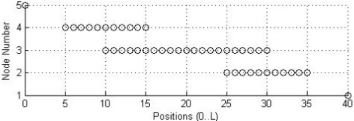
Figure 2.3: The possible positions of nodes x0 to x4 with a slack of 5, in the
example covered in Nielsen et al. (1998).
then the correlationρfor the segment denes the optimal node position x* by
x*=arg maxx N−1 X i=0 ρ(P0[xi;xi+1], T[xi;xi+1]) ! (2.1.11)
=arg maxx Cov(P 0[x i;xi+1], T[xi;xi+1]) p V(P0[x i;xi+1], T[xi;xi+1]) ! (2.1.12) Using this correlation as a penalty function, the optimal solution can be arrived at through dynamic programming. This is done by iterating through all segments starting at x0, keeping the optimal warpings and discarding all
other suboptimal warpings. While sequentially considering the position of every xi (referred to as a node) two matrices are constructed -U, the optimal
warping of each node (numerically between −t..0..t), and F, the cumulative
benet function. Both these matrices have the same dimensions: the number of nodes i along the rows, and all possible node positions along the column -(N + 1)×(L+ 1).
A crucial aspect of the optimisation process is that the benet function is determined for the current node as well as the previous node in the iteration. This optimisation variant is known as backward dynamic programming. An example in the original paper by Nielsen et al. (1998) is based on the following simple warping: L = 40, m = 10 and t = 5, giving three warping segments
with ve nodes in total. The rst (x0) and last (x4) nodes are constrained at
the beginning and ends of signal, and thus x1 and x4 can only be warped 5
positions either way of their origin. The further a node is away from these constraints, however, the more possible warping positions are available due to the cumulative nature of the warping; thus the middle nodes x2 and x3 have
the highest span of possibilities (refer to gure 2.3).
Consider the warping ofx3. Ifx2is placed at position 29 then the position of
x3 is constrained to two values: 34 or 35. Position 34 represents the maximum
warping for the 3rd segment, with warpingu2 = 5andu3 = 4; whereas position
35 is the maximum allowable warping for segment 4 (u2 = 4 and u3 = 5).
Each of these possibilities has a corresponding cumulate benet function value
f([x2, x3]) +f([x3, x4]). The highest of these is the optimal, and is stored in
Once all the nodes have been treated in this way, backtracking throughU
will give the nal optimal warping.
It can be deduced from the above demonstration that the only parameters that are necessary to set are the segment lengthm, and the 'slack't. Extensive
review of the choice of these two parameters, and how they eect the nal correlation between sample and target, is covered in Nielsen et al. (1998). It was determined that the segment length should be set to around the width of the smallest peak in the signal; smaller segments allow for a higher-resolution warping, though do not signicantly add to the nal correlation values. The choice of slack is less dened: the larger the slack, the more possibilities exist for warping and therefore the more computationally intensive the alignment. One therefore needs to nd a balance between alignment exibility and time. Another cost to take into account is over-tting of the data.
It was found by the authors that a slack of just 10% of the segment length was sucient for a reasonable level of accuracy. Anything above this value did not signicantly add to the accuracy of their model alignment, only increasing the computational time gratuitously.
2.1.2.5 Feature Map Alignment
When aligning between multiple measurements along 3 Dimensions, there are two types of approaches (Lange and Tautenhahn, 2008). The rst is know as 'Raw Map Alignment', which is the global correction of retention times across multiple measurements; followed by their superposition and subsequent simultaneous analysis. This type of approach is, however, extremely compu-tationally intensive on a large scale. A second type of approach is known as 'Feature Map Alignment', which usually involves a dewarping step followed by feature detection. Finally, alignment of these features is performed before nal analyses.
In the latter method, 'features' are manifestations of chemical compounds in chemometric data - typically a peak region in retention with a signature along a second dimension (depending on what is attached to the chromato-graphic column). A 'feature map' is the collection of features for a single dataset from a particular run. Generally 'consensus features' are obtained through the feature map alignment process. They represent unique features that are common to feature maps within the larger data set. The 'consensus map' is, in turn the map of these global features.
The existing algorithms and software to achieve the above are almost exclu-sively for cases in which the second dimension is described by the mass-charge ration (m/z) of mass spectroscopy - GC or LC-MS data. There are, however, few to no existing algorithms suitable for the solution of the feature map align-ment problem with HPLC/UV-vis data as is used in this study. Nevertheless, it is still informative to review the existing LC/GC-MS methods as the un-derlying problem remains similar. A brief review of the most prominent of
these methods is presented in a comparative study by Lange and Tautenhahn (2008); the methods and software suites compared remain some of the most commonly used.
Typically, as Lange and Tautenhahn (2008) describes, there are 6 stages of achieving a feature map alignment:
1. Signal pre-processing and centroidisation
2. Detection of the 2-Dimensional features or putative compounds 3. Normalization
4. Warping to correct for drift in retention times
5. Computation of a 'consensus map' by multiple comparisons of features across maps
6. Statistical analysis and interpretation
Items 1 through 4 are explained in the subsection above; 6 in the section below. While there are many dierent methods that can be applied for these steps, they are relatively standard in comparison to the 5th step; for which there are as many algorithms as there are software packages.
Two common distinctions between algorithms are rstly, whether a global correction or 'warping' in retention time is applied (either linear or non-linear); secondly whether clustering or sequential star-wise iteration is used for step 5 above. Notable dangers in feature map alignment are that corresponding features across maps are not grouped into the same consensus feature; secondly that consensus features include multiple features instead of a single unique feature. The most prominent of these software packages, as well as a brief explanation of their approaches, are listed below:
X-Align (Zhang et al., 2005). The algorithm is reliant on pre-dened 'windows', into which detected features are binned for each feature map The most intense feature for each of these windows is then compared across maps; features found in all maps are deemed signicance and an 'average' mapping is created. The map having the features closest to this average mapping is then used as the reference map, to which all other maps are aligned. A nal 'consensus' map is the micro-alignment of all the resultant features.
XCMS (Smith et al., 2006). Part of the R bioconductor package (Gen-tleman et al., 2004). XCMS also employs a window 'binning' technique. Features in the same bin are matched by their mass-spectra signatures. Matching features in the same bin are then resolved using a kernel den-sity estimator, using a probabilistic approach to assign nal nal feature retention times.
msInspect (Bellew et al., 2006). Combines the features from multiple experiments into what it calls a single 'peptide array'. It is assumed that warping in the measurements occurs due to a global linear eect, which is rst estimated using the most intense features with similar m/z values. After warping according to this linear transformation, it uses a method of 'divisive clustering' to compare and assign the features into the nal peptide array. User-dened parameters to achieve this include a window threshold for both retention time and m/z ratio.
MZmine (Katajamaa et al., 2006). The method used in this software is subtly dierent from the ones above due to the fact that it does not assume a global trend from which individual experiments must be de-warped. Rather, a 'master list' of features is created. Each map is compared in turn to this master list of features within a retention time window; if the compared feature is deemed similar to the master feature according a set tolerance (both in retention time or m/z value) using some similarity score, the feature is assigned to the master feature. If not, it is appended to the master list as a new feature. The nal consensus map becomes this master list once the analysis is complete.
Lange and Tautenhahn (2008) performed quality checks on all of the above methods by obtaining a 'ground truth' of consensus feature maps using MS/MS data that was excluded from the respective software's analysis. The nal results from each software suite was then compared to the ground truth in two ways: rstly precision, the probability that an assigned feature is correct; secondly recall, the probability that an assigned feature is found.
This comparison was performed on both protein and metabolic-centric data sets. For the latter, MZmine generally performed best according to both mea-sures.
A more recently developed implementation is an iteration of peak map alignment in PyMS. The algorithm employs an unsupervised clustering tech-nique; building a tree-like structure from feature maps and performing a bottom-up alignment (Isaac et al., 2012). It relies on a 'common ion' to indi-cate similarity between features in dierent data sets; once again precluding its use with the UV-vis data at hand. No comparisons in literature of this method with the aforementioned were found; however there does appear to be conceptual promise in this unbiased approach.
2.1.3 Machine Learning Techniques
The analysis of data processed by the above means should be statistically analysed for both the purpose of validation and hypothesis generation for the un-targeted analysis. To this end, several machine learning techniques can be applied; namely, decision trees, principal component analysis and network analysis methods.
2.1.3.1 Decision Trees
Decision trees are one of the most popular machine learning methods for clas-sifying data (Rokach and Maimon, 2005). They are consistently used for their easy interpretability; simplicity and the fact that little to no preprocessing is necessary on the data. It sequentially divides the data into discrete classes using optimal binary partitioning, based on some metric. This process constructs a network in the form of a directed tree. The nodes or 'leaves' -represent classes, while the edges ('branches') are partitions of the data. Each branch is created from a test on one of the variables in the input data. The test will result in a binary split.
At the top of the decision tree is the rst variable criterion by which the data is split - at the bottom are the nal class assignments once the model has reached its conclusion. Each level of the tree from the apex downward constitutes a renement of the model - a lower mis-classication rate - until the data is classied with perfect delity. This top-down approach is known as 'recursive partitioning'; and this type of algorithm is greedy - aggressively nding local optima, aiming for a globally optimum solution (Rokach and Maimon, 2005).
The metric by which the variable test is chosen is most commonly the gini index. The gini index measures the divergent probabilities of the binary split in the data based on a given variable test. Concretely, it is the likelihood that a random sample will be mis-classied within its sample subset at that point in the tree, given all the previous binary conditions.
If samples can take on class labels(1..m), andfi is the number of samples
with label i in the data subset at that point in the tree, then the probability
that it is misclassied at that point is as follows:
P = m X i=1 fi(1−fi) = 1− m X i=1 fi2 (2.1.13)
This heuristic is greedily estimated for all possible variable splits at each level; in this way the algorithm is NP-complete, which can become restrictive with large scale data.
A useful aspect of decision trees lies in the ability to determine a quick variable importance metric from the model. This is known as gini importance, and is calculated for each variable by simply adding up the reduction in gini impurity at each branch in which the variable is the tested.
This measure has already been used to good eect in chemometrics by Menze and Kelm (2009) for feature selection on several spectral data sets, using random forests - essentially an ensemble method combining multiple decision tree models.
2.1.3.2 Principal Component Analysis
Principal component analysis is a ubiquitous method for data mining in chemo-metrics (Wold et al., 1987). It is most often used for the purposes of clustering as well as the discovery of new- or validation of known latent variables in data. At its base, it is a technique that maps a dataset from its existing set of variables onto a new set of axes or 'principal components'. These new axes coincide with the direction of most variance within the data set, in decreasing order; in this way they form an orthogonal set of vectors.
Typically only a few of these principal components are needed to explain most of the data's variance, so that the dimensionality is greatly decreased. It is often found that the rst few components are reective of latent variables. The process of mapping the data onto principal components results in two useful matrices: the loading and score matrices. The scores are essentially the distance of each sample from the principal components; the loadings are vectors of the relative 'direction', or transformation from each of the original variables to the principal components.
The scores are useful in deriving how principal components relate to latent variables, while the loadings inform how original variables inuence the prin-cipal components; combining these two sources of information, one can draw qualitative and quantitative conclusions as to how original variables inuence latent variables.
2.1.3.3 Network Analysis
Networks are a relatively novel tool in the analysis of metabolomic data on a large scale. Recent work by Jacobson et al. (2013) used a method of network reconstruction to represent underlying chemical reactions in the aging of port wine. Seeing that the data used in this study is also wine-related and time-series based, much the same techniques were applied for statistical analysis on the nal preprocessed data. Network reconstruction is particularly useful for the un-targeted approach used, as it maps out the underlying chemical relationships between detected features in a manner that is visually stimulating to the analyst, aiding in hypothesis generation.
Networks have the ability to model the correlation between chemical fea-tures. A simple metric such as Pearson correlation can be used, although the method is open to other statistical metrics should these be more applicable. An all-against-all calculation of correlation can then be performed between features. The nodes of the networks thus consisted of the features; while the edges were weighted by the correlations between them.
Two ways of depicting the resultant network is either to make an arbitrary threshold of correlation, so that only the signicant interactions are shown; or constructing a Maximum Spanning Tree (Jacobson et al., 2013). While the former is capable of showing a more complete view of the interactions in a
data set, its interpretability can suer from an abundance of information. In this way, a Maximum Spanning Tree can reduce the data set to only its most salient components, and in so doing represent the skeleton of the network's strongest lines of communication.
A Maximum Spanning Tree is simply the inverse of a Minimum Spanning Tree, a network construct often seen in literature - originally for the solution of the classic 'Travelling Salesman' problem (Kruskal, 1956). A spanning tree is a subgraph of any connected graph in which there are no cycles, and all nodes within the graph are connected. In weighted graphs, the Minimum Spanning Tree is the spanning tree for which the overall sum of edge weights is the minimum possible.
The same algorithm devised by Kruskal is used; the inverse of the edge weights are simply taken. Briey, the algorithm works as follows (Kruskal, 1956): rstly, a 'forest' is initialised from the graph at hand by adding each individual node as a separate tree. A set of all the edges from the original graph is then created. At each iteration, the edge with minimum weight is removed from this set. If this edge connects two of the trees in the forest, it is included into the growing minimum spanning tree; else it is discarded. The iterations cease once all nodes are connected (there is only a single tree in the former forest).
Jacobson et al. (2013) stated that a further advantage of the Maximum Spanning Tree when applied to models of chemical reactions is that it is ro-bust to missing data - intermediate steps within chemical reactions are not reected in the tree as the strongest correlations over time will be between initial substrates and nal products. Additionally, it was proposed that with time-series data the maximum spanning tree has a kinetic element; the ow through the tree representing consecutive reactions in a directed chemical evo-lution of the media.
2.2 StatNet Literature
2.2.1 Background
Wong and Bergeron (1994) compiled an historical review of the advancement of scientic visualisation, especially regarding that of multi-dimensional, mul-tivariate data (MDMV). The rst stage of analysis, dubbed the 'Searching Stage', was characterised by small datasets usually visualised in 2-dimensional plots, occasionally augmented by other graphics denoting categories (in one case the display of cartoon faces with diering expressions on each data point). The second stage of data analysis ('The Awakening', assigned to the years 1977-1985), was fomented by Tukey's exploratory data analysis (EDA). This was more a foundational paradigm, as enshrined by a brief paper entitled 'We Need Exploratory and Conrmatory' (Tukey, 1980). The principal idea
behind this movement was to generate hypotheses instead of only conrming pre-existing ones. Naturally, the visualisation of experimental results was at the center of this ideal. This stage was also aligned with the advancement of computing power, and the advent of the personal computer, allowing for widespread adoption and development of techniques related to EDA. The data sets were generally two- or three dimensional at most; however many of the techniques developed remain the most prevalent today.
Included in Tukey's book on EDA (Tukey, 1977) are typical graphical ex-ploratory techniques; ones that are still applied today with great success. Ex-amples include boxplots, histograms, pareto charts, scatter plots, and stem-and-leaf plots. All of these methods draw their power from classical statistical measures, by which they are dened.
Wong et al. describe the third stage of scientic visualisation (1986-1991) as that of discovery. Studies into interpretation of mdmv data moved away from statistical metrics in two dimensions, and attempted to describe all dimensions of the data in a single plot. This type of analysis relies heavily on the drive of graphical computing, which was gradually facilitating this shift. The nal stage was described, at that time, as being one of elaboration - combining the techniques developed up to that time into new methods.
Although there have been many advances in the eld of visualisation, in the interpretation of experimental results often the simplest methods are still employed. The plotting of several overlaid line graphs over a time axis; surface response plots and bar graphs are still prevalent in literature.
2.2.2 Network Visualisation
Networks have been used extensively in the eld of data visualisation. A review of the various manifestations of networks in this realm is done by Herman et al. (2000). The author claims that most information systems in which there are inherent relationships between data elements are susceptible to being rendered into a network.
The application areas listed, however, are generally dened by relationships of extant - not putative - knowledge. Included are systems of predetermined interactions such as computer ling systems; object-oriented programming rep-resentations such as UML diagrams and various other hierarchical formats. In addition to this, biology is a eld at the fore of large-scale network analysis for phylogenetics; biochemical pathways; metabolomics and genomics.
Probably the most prevalent example of network visualisation for data mining is that of decision trees (Rokach and Maimon, 2005). This machine-learning technique is typically applied to high-dimensional data sets in order build a supervised model of the data and ascertain which variables are most signicant towards the prediction of a (single) outcome. In simplistic data sets, the application of this method would not lead to sensible results; it is more appropriate for large-scale data sets.
Some of the concepts within decision trees may, however, be applicable. The topography of a decision tree - with inputs leading from a root node to leaves representing the outputs - is a fundamentally concise and representative way of presenting relationships for dependent data.
2.2.3 Temporal Data
Two of the three experimental data sets analysed in this study were based on time-series (temporal) data. As one of several fundamental types of data (Shneiderman, 1996) it often requires distinct methods for its presentation. Aigner et al. (2008) performed a review on contemporary methods for visu-alising time data specically. The authors distinguish between analyses that include time as an incidental variable, or simply integrate it into the depiction of others. The latter is more common for scientic analysis; the former for the purposes of planning.
Furthermore, three important distinguishing factors are listed for visual-isation of temporal data: rstly, whether the time measurement is linear or cyclical. Both instances of the temporal data analysed were linear; the most common and easiest to visualise. The second distinction is whether the data involves discrete time points or time intervals; only the former is used in the current study. The last is whether time is organised or branches; branching cases were not encountered in the current development.
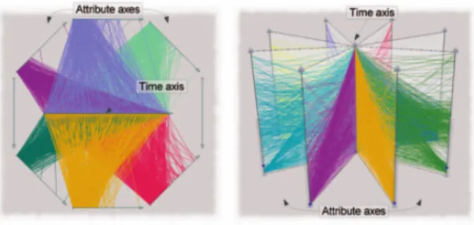
According to these criteria, the most applicable method covered by the authors is 'TimeWheel' analysis (Tominski et al., 2004). This analysis relies on a 2-Dimensional multi-axis view. Time occupies a central axis, around which axes related to output variables are evenly spaced, reminiscent of the spokes of a wheel. At each discrete time point (the method does not lend itself to time intervals), a line is drawn between its position on the temporal axis and the corresponding level on the variable axis. For each attribute, therefore, the uctuation of an attribute over time can be characterised the relation to the central axis; for example - if the attribute decreases over time, the formation of the parallel lines will be upper-triangular; if the opposite is true it will be lower triangular (depending on the orientation of the time axis).
There is value to combining several attribute graphs in this way, however the inclusion of so many parallel lines can be overwhelming to the end-user. While the overall trend may be characterised, it is dicult to identify poten-tially interesting edge cases. All of the data is included in the visualisation, making the method exhaustive, but there is no elimination of insignicant comparisons.
Although it may not be the express purpose of the technique, visualising experimental data where there are perturbed variables and several measured outputs remains dicult. Essentially these are two conceptual layers in the data - an 'input' and 'output' paradigm which is challenging to view simulta-neously.
Figure 2.4: Time Wheel Method for visualising temporal data as depicted in Aigner et al. (2008)
2.2.4 Principal Component Analysis
Probably the most prevalent technique, however, in visualising and interpreting high-dimensional data is Principal Component Analysis. This has the ability to reduce the pertinent information in a multivariate data set into a few com-ponents that can be analysed in 2-dimensional plots. The technique itself is discussed more fully in section 2.1.3.2; however, many of the interactions and subtleties between variables in a data set are often not suciently described in loading plots. In data sets with relatively small numbers of variables, this technique also loses it's power of description; often classical visualisations from the above-mentioned second stage of development (line graphs, box plots and surface plots) are reverted to in order to describe outcomes.
2.2.5 Data Interaction
While the nature of how data is presented is the primary concern in inter-pretation, an important augmentation of any visualisation is the ability to interact with the results. Keim (2002) summarised the various ways in which interactive data representation can assist in visualisation.
The rst is 'dynamic projection'. This includes methods of projecting high-dimensional data onto low-dimensional spaces in order to render the information amenable to human interpretation, which is at most capable of three dimensions. The most prevalent of these techniques it the 'Grand Tour' method, which projects subsequent representations of high-dimensional scatter plots onto 2-dimensional planes.
Another aspect of interactivity is the ability to lter the data. Splitting the data into subsets is an extremely useful tool for any end-user; the ability to extract meaningful segments from the overall analysis to arrive at logical syllogisms. These can also be dened as advanced data 'queries' that reect specic questions related to the data. Consummate with ltering should be an automated re-organisation of the visualisation so that interpretability is retained.
The third factor listed by Keim (2002) is interactive zooming. The visu-alisation should have an overarching structure from which conclusions can be drawn; however, users should have the freedom to focus on particular areas of interest, so that detailed conclusions can be drawn.
Two further types of data interactivity are interactive distortion (simulta-neous presentation of diering levels of detail) and interactive linking (combi-nations of disparate visualisation techniques); neither of which are applicable to the present method.
2.2.6 Statistical Methods
The statistical methods used in StatNet are relatively straightforward. Most of the power of visualisation lies in the topographical structure of a network than in the descriptive ability of the statistics themselves. Nevertheless, an overview of the statistical measures, tests and corrections is discussed below. 2.2.6.1 Metrics
The metrics used to quantify the relationships in the data were generally either fold change and Pearson correlation. Fold change F is simply the symmetrical
ratio of two measures a and b; such that their relative change is centered at 1
and -1: r= a b;F = ( r :r≥1 −1 r :r <1 ) (2.2.1) Pearson correlation is dened by the familiar equation; the ratio between co-variance and combined standard deviations:
ρX,Y =
Cov(X, Y) σXσY
(2.2.2) Where covariance is dened as the combined expected deviations from respec-tive means:
E[(X−µX) (Y −µY)] (2.2.3)
2.2.6.2 Statistical Tests
Dierent tests are appropriate to determine signicance for variable com-parison, depending on whether an underlying probability distribution is as-sumed; and if so, which distribution. Two examples of a parametric and non-parametric test are illustrated below.
In general for testing of signicance dierences where a normal distribu-tion is assumed, a Student's t-test can be used. The T-Test is used for normal
distributions, and has the advantages of speed and ease of application. The t-statistic is given by the following equation for the comparison of two inde-pendent samples of identical length n:
t = X1−X2 sX1X2 · r 2 n (2.2.4) where sX1X2 = r 1 2 s 2 X1 +s 2 X2 (2.2.5)
sX1X2 is the pooled standard deviation; s
2
X1 and s
2
X2 estimators of the
vari-ances of the two samples respectively. This is essentially a normalisation for the combined samples.
This t-statistic is assumed to follow a normal distribution. A test is there-fore performed at the requisite dened thresholds in the normal distribution to establish whether the null hypothesis - that the samples' means are not signicantly dierent - is true.
A non-parametric alternative to the t-test can also be used, especially when the vectors being compared were of a small length N. This was in the form
of the Wilcoxon Rank Sum test (Wilcoxon, 1945). Its appeal is that the only assumptions needed in order to perform the test was that the samples are randomly drawn from the same population and are amenable to sorting - i.e. they vectors have an ordinal scale.
The test compares the requisite pairs of values (x1,iandx2,i) for each sample
in the ordinal ranking. For each one of these pairs ini= 1..N,|x2,i−x2,i|and
sgn(x2,i−x1,i) are calculated. The Nr pairs are then ranked by the absolute
dierence measure, after which the test statistic W is calculated: W =|
Nr X
i=1
[sgn(x2,i−x1,i)·Ri]| (2.2.6)
The null hypothesis is then rejected ifW is below a set threshold, as is the
case with the p-value generated from the t-test.
2.2.6.3 Correction for Multiple Hypothesis Testing
The danger in making many simultaneous hypothesis tests is that it is possible to propagate false positives, or 'Type 1' errors. This is also known as familywise error rate (FWER). A correction for this is in the form of the Holm-Bonferroni Correction (Holm, 1979). It is based on the Bonferroni Correction method, but is cited by Holm et al. as being statistically more powerful.
The multiple hypotheses are corrected by rst rank-ordering the p-values
sequentially in order of lowest to highest; at each iteration the probabilityPkis
compared to a new probability threshold, adjusted from the original as follows:
Pk >
α
m+ 1−k (2.2.7)
Where α is the selected signicance level. If a p-value fails this test along
the bottom-up search, all subsequent hypotheses with higher p-values are voided and the algorithm terminates.
2.3 Conclusion
A body of literature has been reviewed to establish a platform for untargeted chemometric analysis and network visualisation.
In terms of model data for untargeted chemometric analysis, HPLC/UV-vis is a good candidate for novel methods. The data generated by the extensive experiments into browning phenomena by (Buica, 2012) is conserved, has ex-perimental duplicates and presents an interesting challenge due to its scale and diversity of experimental conditions. There are also clear targets for building models of the data, in the form of distinct classes of experimental variables.
After reviewing a number of pre-processing techniques, it is proposed that the following should be incorporated into a large-scale analysis: smoothing using the standard Savitzgy-Golay lter (Savitzky and Golay, 1964); base-line correction using wavelet methods as implemented in the alignDE package (Zhang et al., 2011) and peak alignment using the simple yet eective COW (Tomasi et al., 2004).
HPLC/UV-vis data has a rich feature map, with continuous features along wavelengths. Untargeted analysis using the full map is something not often attempted, and may yield useful results. The incorporation of information across both dimensions would be preferable as features can dier across wave-lengths. As feature map alignment algorithms are generally only implemented for discrete MS data, a new implementation would need to be developed that is memory ecient and can be applied sequentially for a group of UV-vis chro-matograms. A brief review of some of the more prominent MS implementations was expounded; the closest method to the stated requirements is most likely MZmine as developed by (Katajamaa et al., 2006).
Several candidate machine learning and statistical methods were reviewed, the applications of which to the results of an untargeted analysis may give insight and validation.
Opportunities for the application of network methods were also explored. While there has been much progress in the eld of exploratory data analysis and visualisation, there is still room for new methods to explore the multivari-ate space of scientic experimentation - especially with temporal data, which has an added layer of complexity.
Pure network representations are not often applied to this eld, but rather used as a motif for conceptual design. It may be possible to employ networks as a multivariate comparison tool for hypothesis generation using experimental results. Several statistical metrics for feature comparison were also reviewed as possible bases for network visualisations.