A Multi-Objective and Evolutionary Hyper-Heuristic
Applied to the Integration and Test Order Problem
Giovani Guizzo∗, Silvia R. Vergilio, Aurora T. R. Pozo, Gian M. Fritsche DInf - Federal University of Parana, CP: 19081, CEP 19031-970, Curitiba, Brazil
Abstract
The field of Search-Based Software Engineering (SBSE) has widely utilized Multi-Objective Evolutionary Algorithms (MOEAs) to solve complex software engineering problems. However, the use of such algorithms can be a hard task for the software engineer, mainly due to the significant range of parameter and algorithm choices. To help in this task, the use of Hyper-heuristics is recom-mended. Hyper-heuristics can select or generate low-level heuristics while opti-mization algorithms are executed, and thus can be generically applied. Despite their benefits, we find only a few works using hyper-heuristics in the SBSE field. Considering this fact, we describe HITO, aHyper-heuristic for the Integration and Test Order problem, to adaptively select search operators while MOEAs are executed using one of the selection methods: Choice Function and Multi-Armed Bandit. The experimental results show that HITO can outperform the tradi-tional MOEAs NSGA-II and MOEA/DD. HITO is also a generic algorithm, since the user does not need to select crossover and mutation operators, nor adjust their parameters.
Keywords: Metaheuristic, Hyper-heuristic, multi-objective algorithm, search-based software engineering, software testing
∗Corresponding author
Email addresses: [email protected](Giovani Guizzo),[email protected] (Silvia R. Vergilio),[email protected](Aurora T. R. Pozo),[email protected] (Gian M. Fritsche)
1. Introduction
Search-Based algorithms have been successfully applied to solve hard soft-ware engineering problems in the field of Search-Based Softsoft-ware Engineering (SBSE) [23]. Some of the most used algorithms in SBSE are Multi-Objective Evolutionary Algorithms (MOEAs). Such algorithms are based on Pareto
dom-5
inance concepts and offer to the user a set of good solutions that represent the best trade-off between different objectives, which, in software engineering, are generally associated to software metrics to evaluate the quality of a solution.
However, the usage of a MOEA is not always easy for the software engi-neer. Many times, it demands effort to adapt implementation details, to adjust
10
parameters (e.g. mutation and crossover probabilities), to select search-based operators, and so on. Another difficulty is that some of them are adjusted, de-signed or evaluated for a specific problem, which can affect their generality [8]. To overcome these limitations, the hyper-heuristic field has emerged. A hyper-heuristic is a methodology to automate the design and tuning of heuristic
15
methods to solve hard computational search problems [9]. It is used to select or generate newlow-level heuristics (LLHs) while algorithms are being executed. The idea is to provide more generally applicable and flexible algorithms, while yielding better results than conventional algorithms alone. A distinctive charac-teristic of hyper-heuristics is that they operate over the heuristic space instead
20
of the solution space. This can be interpreted as a technique to select or generate the best heuristic that solves the problem, instead of solving the problem di-rectly [8]. To allow this, a hyper-heuristic dynamically guides the search process by managing a set of LLHs (e.g. metaheuristics and genetic operators).
The usage of such methodology in SBSE has raised interest. Harman et
25
al. [22] state that hyper-heuristics can contribute to obtain holistic and generic SBSE algorithms. However, we can find few works applying hyper-heuristic in SBSE [6, 27, 31, 37]. Motivated by this, we introduced HITO in [21], a
Hyper-Heuristic for the Integration and Test Order Problem.
The Integration and Test Order Problem (ITO) consists in generating an
order for the units (the smallest part of a software) to be integrated and tested, in a way that the stubbing cost is minimized [4]. A stub is an emulation of a unit that is not yet implemented, tested or integrated in the software. Therefore, a unit that is required by another unit shall be emulated to enable a proper testing or integration. The underlying cost of this problem is the potentially great
35
number of stubs that may be generated during the testing activity. These stubs will be obsolete once the emulated units are implemented, and consequently, such stubs become wasted resources. By rearranging the unit ordering, we can force the most required units to be integrated and tested first, so that the next units will not require a stub for such a unit. This problem has some
40
characteristics that make it suitable for application of hyper-heuristics [21]. The cost is impacted by different factors, such as size/complexity/number of classes, methods, attributes, return types, parameter types, and any other element that must be emulated in order to proceed with the integration and testing. Hence multi-objective algorithms have presented good results [4]. It is possible to use
45
several search operators and the problem is found in several contexts such as object- and aspect-oriented testing, thus, it may be configured in several ways. To allow a proper, generic and efficient solution to the ITO problem, HITO uses a selection method and a novel rewarding measure to select the best LLH (combination of crossover and mutation operators) at each evolutionary mating.
50
By using HITO the software engineer does not need to select the crossover and mutation operators to be used by the MOEAs. He/she does not need to choose the probabilities for these operators.
HITO was designed to be flexible and robust, hence it has the following main characteristics: i) a set of steps to select and apply LLHs using MOEAs; ii) a
55
set of parameters to allow the user to personalize its functionality; iii) selection of the best LLH at each mating, in contrast to other works (such as [28, 31, 36]) that perform the selection at each generation; iv) a rewarding function that is based on the Pareto dominance concept and uses solely the parents and children involved in the mating, rather than using quality indicators such as in [36]; v)
60
Bandit (MAB) [19], which can also be chosen by the user. We acknowledge that these characteristics can help HITO in overcoming the limitations of MOEAs and also obtaining the best results. Preliminary results [21] proved that HITO is capable of solving real instances of the ITO problem.
65
Considering the HITO advantages and its promising results, this work ex-tends [21] by providing a better description and a deep analysis of HITO with new experimental results. We can mention the following contributions:
• We propose an improved reward measure that was redesigned to encom-pass different numbers of parents and children involved in the mating (e.g.
70
generating one child or generating two children);
• We present results from a broader evaluation encompassing two quality indicators, two statistical tests, a set of many objective functions, three versions of HITO (using MAB, CF and a random selection strategy), and two conventional MOEAS: i) NSGA-II: well-known and widely applied in
75
SBSE.; and ii) MOEA/DD: state of the art algorithm for multi-objective problems. This new empirical evaluation was conducted to improve the accuracy of the evaluation of HITO, and to assess not only how well it performs when compared to conventional algorithms, but also to assess if a random LLH selection is enough for this problem;
80
• We use four different objective functions to analyze how a selection hyper-heuristic such as HITO behaves with many objectives. The experimenta-tion shows favorable results for all considered systems.
In the experimentation we used two sets of objective functions to evaluate the solutions: a set based on two metrics (number of attributes and number
85
of methods to be emulated), and a set based on four metrics (number of at-tributes, number of methods, number of return types, and number of parameter types to be emulated). These are the same objective functions used in previ-ous works [4, 21, 37]. Furthermore, we applied the algorithms on 7 real world object-oriented and aspect-oriented systems. These are well known and widely
used systems [4, 3, 21, 47, 37, 48], with different characteristics and varying in size (lines of code, number of classes, etc). The results are favorable for HITO in terms of quality indicators and statistical analysis. HITO was able, in overall, to outperform all the MOEAs with statistical significance, while being outperformed by MOEA/DD in only one system.
95
This work is organized as follows: Section 2 contains a brief explanation of hyper-heuristics, their main components and the selection methods used in this work. Section 3 reviews the ITO problem. Section 4 presents related work; Section 5 presents a detailed description of HITO, the reward measure being proposed, the LLHs, the credit assignment measures and the adapted selection
100
methods implemented in this work. Section 6 describes and analyses empiri-cal results from HITO evaluation. Finally, Section 7 presents the concluding remarks and future works.
2. Hyper-Heuristics
Hyper-heuristics are often defined as “heuristics to select or generate
heuris-105
tics” [9]. A hyper-heuristic may be used to select the most appropriate heuristics or to generate new heuristics using existing ones. Chakhlevitch and Cowling [10] define hyper-heuristics as higher level heuristics that: i) manages a set of LLHs; ii) searches for a good method to solve a problem rather than searching for a good solution; and iii) uses only limited problem-specific information.
110
The goal is to find the right method or sequence of heuristics to be used in a given situation rather than trying to directly solve the problem [8]. Thereby, one of the main ideas is to develop algorithms that are generally applicable in several problem instances [8]. By achieving that generality, the algorithm may be used with less human effort and additionally to obtain better results. This idea was
115
motivated by the difficulties regarding the application of conventional search techniques, such as the great number of parameters for configuring algorithms and the lack of guidance on how to select the right LLHs [8].
by the hyper-heuristic approaches [10]. The idea is to maintain a “domain
120
barrier” that channelizes and filters the domain information visible by the hyper-heuristics. In other words, the hyper-heuristic should be independent of the problem domain by only having access to some domain-independent information from the domain barrier [9, 10].
In this paper we use the hyper-heuristic definition given by Burke et al. [9]:
125
“A hyper-heuristic is an automated methodology for selecting or generating heuristics to solve hard computational search problems”. The authors also pro-posed a classification for hyper-heuristics as seen in Figure 1. We can see two main dimensions [9]: i) the heuristic search space nature; and ii) the sources of heuristic feedback. The heuristic search space nature defines if a hyper-heuristic
130
is either used to: i) select existing LLHs; or ii) generate LLHs using components of existing ones. In this categorization there is a second level dimension that is concerned with the nature of the LLHs used by the hyper-heuristic: i) con-struction; or ii) perturbation. The construction heuristics start with an empty solution, and gradually build a complete solution. On the other hand, the
per-135
turbation heuristics start with a complete solution (either randomly generated or gradually built by construction heuristics) and try to iteratively improve it.
Figure 1: Classification of hyper-heuristic approaches according to [9]. Extracted from [9].
The second dimension is the source of heuristic feedback [9]. The learning hyper-heuristics can be divided into two categories: i) offline learning; and ii) online learning. Offline learning hyper-heuristics gather knowledge from a set
140
of training instances, and use this knowledge to generalize the solving of unseen instances. Online hyper-heuristics use online information about the performance of LLHs to dynamically select them, thus it is potentially more flexible than offline approaches. There are also non-learning hyper-heuristics (e.g. random) that simply do not use feedback to guide the search.
145
In this paper we work with a hyper-heuristic for online selection of perturba-tion LLHs, more specifically for selecting search operators for Multi-Objective
Evolutionary Algorithms (MOEAs) [11]. Selection hyper-heuristics use two main components [8]: i) heuristic selection method; and ii) move acceptance method. In addition, each of these methods can vary independently, which
150
brings more generality to the hyper-heuristic approaches. A selection method uses techniques to select a LLH in a given moment of the search, either using a learning or a non-learning approach, whereas the move acceptance method decides whether a solution obtained by the selected LLH must be accepted.
The hyper-heuristic presented here uses two score-based heuristic selection
155
methods: Choice Function (CF) [12] and Multi-Armed Bandit (MAB) [19].
2.1. Choice Function
The Choice Function (CF) adaptively ranks the LLHs according to their previous performances [12]. CF was proposed initially to select LLHs based on their scores and using several strategies in order to solve the Scheduling Sales
160
Summit combinatorial problem. The promising results of the authors motivated other works to use CF as a selection method, such as [29, 36].
The credit assignment equation of CF is formulated according to the works of Cowling et al. [12] and Kendall et al. [29], and was presented as follows:
f(hi) =αf1(hi) +βf2(hi, hj) +δf3(hi) (1)
wherehi is the LLH being evaluated;hj is the LLH that has just been applied; f1(hi)is the recent improvement ofhi;f2(hj, hi)is the recent improvement ofhi when called immediately afterhj;f3counts the CPU seconds that have passed
165
sincehiwas last called; and the variablesα,β andδare the weight parameters in the interval [0,1] for the functionsf1,f2andf3respectively.
In Equation 1, the functionsf1 andf2are used for intensification purposes, i.e., for a better exploitation of the search space by favoring the LLHs that have been yielding the best results so far [29]. In contrast, f3 is used for the
170
diversification of the solutions, i.e., for a better exploration of the search space by favoring LLHs that have not been applied in a while. These functions and their weight parameters were introduced in the equation to balance the search
between the intensification and diversification factors. If a greater intensification is desired, thenαmust be increased, or decreased otherwise.
175
Equation 2 shows a simplified version of the credit assignment of CF used in [36]. This version contains only two functions: f1 andf2.
f(h) =αf1(h) +βf2(h) (2)
wheref(h) gives a score for a LLHh;f1 reflects the recent improvement ofh; f2 is the elapsed CPU seconds since hhas been called; and αand β are the weight parameters to balance the values off1 andf2.
We use in this work the adaptation of CF proposed by Maashi et al. [36] due to its promising results and easy usage. We propose a different mechanism
180
to evaluate LLH improvements using solely the concept of Pareto dominance as f1 and elapsed iterations asf2. We adopted these changes in order to design a CF more compatible with HITO.
2.2. Multi-Armed Bandit
Auer et al. [5] proposed theUpper Confidence Bound (UCB)selection
strat-185
egy inspired by the Multi-Armed Bandit (MAB) problem [5, 19, 33]. In this problem there is a set of K independent arms and each arm has an unknown probability of giving a reward. The goal is to maximize the accumulated reward by pulling the arms in an optimal sequence. Other works such as [13, 19, 24, 35] proposed new algorithms to adaptively select operators using the MAB and
190
UCB inspiration. In this work, we call UCB as MAB method, and the other MAB based selection methods as a derivation of the MAB method.
The idea behind the MAB method is that a given operator i is associated to two main values [5, 19]: i) an estimated empirical reward qˆi that measures the empirical reward of the operator over time; and ii) a confidence interval, depending on the number of times the operator was executed. The MAB method selects the operator with the best value according to Equation 3 [19]:
arg max i∈I qˆi+C r 2 logn ni ! (3)
where i is the i-th operator of a set of operators I; qˆi is the average reward obtained byi so far;C is the scaling factor parameter, i.e., controls the trade-off between the exploration and exploitation;nis the overall number of operator
195
executions so far; andni is the number of times the operatoriwas executed. Originally, the scaling factorCwas not introduced in the MAB equation [5], but was proposed by Fialho et al. [18] to balance the scales of exploration and exploitation. If the exploration is desired, then theC parameter must be increased. However, if exploitation is desired, then C must be decreased. In
200
essence, other adaptations of the MAB method vary the computing of qˆi and ni (i.e. credit assignment and memory length), while maintaining the heuristic selection as themax value for Equation 3.
In this paper we use a variation of the original MAB method, which is called Sliding Multi-Armed Bandit (SlMAB) proposed in [19]. This strategy
205
introduces a memory length adjustment and a credit assignment function that allow a faster identification of changes on the performance of LLHs. Because of this, we decided to use SlMAB in this paper.
The SlMAB credit assignment uses two main functions to compute the score of a given operator. Equation 4 shows how SlMAB computes the reward esti-mateqˆi, which corresponds to the exploitation factor:
ˆ qi,t+1= ˆqi,t W W+ (t−ti) +ri,t 1 ni,t+ 1 (4)
whereiis thei-th operator;tis the current time step (e.g. algorithm iteration or generation);ti is the last time step in whichiwas applied; W is the size of
210
thesliding window;ri,t is the instant/raw reward given to the operatoriat the time stept; andni,t is the number of timesiwas applied until the time stept. The key element in this equation is the introduction of a sliding window of sizeW, which is the memory length. A sliding window is a type of memory that stores the lastW rewards obtained by the operators. These values are used to
215
compute the quality of the operator. This can be done in several ways, but in this work we use the extreme credit assignment, which defines the reward of an operator as the best reward found in the sliding window. We adopted this
strategy because Fialho et al. [19] concluded that it is the most robust operator selection method in combination with SlMAB.
220
The second function (described in Equation 5), which composes the credit assignment component of SlMAB, is used to compute the exploration factor.
ni,t+1=ni,t W W + (t−ti) + 1 ni,t+ 1 (5)
whereni,t is the application frequency of iuntil the time stept; and the other variables are the same as the previous equation.
This equation demands a counter ni,t for storing the application frequency for each operator. This credit assignment is later used in Equation 3, where the operator that maximizes the equation is chosen to be applied.
225
The good learning capability of MAB and its results in other works [19, 35] are our main motivations for its usage. Furthermore, we expect that this method properly guides the hyper-heuristic search with more accuracy than CF, due to its mechanisms designed for a continuous learning. We adapted the SlMAB implementation in order to make it more compatible with the hyper-heuristic
230
proposed in this paper. The adaptations of CF and SlMAB can be seen in Sections 5.3 and 5.4 respectively.
3. The Integration and Test Order Problem
The unit test focuses on testing the smallest part of the program. However, a software usually has several units that must be integrated and tested in order
235
to reveal interaction problems between them. This activity, called integration testing, sometimes requires the creation of stubs. A stub is an emulation of a unit that is created when such unit is required by other units, but it is not yet available. The problem in creating stubs is that the development of these artifacts is error-prone and costly [48]. Therefore, minimizing stubbing costs
240
is fundamental to reduce the testing efforts and costs. This minimization can be done by finding an optimal sequence of software units for integration and testing, which is the problem known as ITO problem.
The ITO problem is found in different development contexts [4], such as: i) component-based [26]; ii) object-oriented (OO) [4, 48]; iii) aspect-oriented
245
(AO) [4]; and iv) software product lines [25]. Nevertheless, to represent units and their interdependencies, one may use different kinds of models, such as graphs, Test Dependency Graphs (TDG) [45], and Object Relation Diagrams
(ORD) [32]. The latter is the most used for OO and AO contexts [48]. An ORD of a system contains its classes, interfaces and their interdependencies modeled
250
as a graph, where the classes and interfaces are the vertices and the dependencies are the edges. The ORD graphs are represented by data matrices that are used by the algorithms to compute the cost of each unit sequence. In this paper we use an extension of ORD (proposed in [4]) to include the AO components in this graph, such as aspects, advices and join points. This allows the execution
255
of algorithms previously used only in OO context, for AO systems. In addition, based on the results of [4], we use a combinatorial approach in which classes and aspects are all integrated and tested together.
In other contexts the tester must be concerned about how many dependency cycles he/she must break in order to minimize the test cost. If a cycle is broken,
260
then a stub must be created to fulfill the dependency. When there are no cycles in the dependency graph, then a simple inverse topological sort of the graph can find a solution that does not require stubs [4]. On the other hand, if a dependency graph has many cycles, then the problem becomes complex and search-based algorithms are applicable to find good orders. Some SBSE works
265
have applied metaheuristics to solve this problem [4, 7, 47, 48].
We choose to tackle this problem due to its main characteristics that al-low a robust application of hyper-heuristics: i) it is properly solved by multi-objective algorithms [3, 4, 47]; ii) the representation of the problem is the same as permutation problems, which provides several operators to be selected by the
270
hyper-heuristic; iii) the problem can be addressed in several contexts; and iv) it is a real problem, hence if effectively solved, the engineer effort invested in this activity can be significantly reduced. In this sense, the objective of applying hyper-heuristics in this work is to provide a generic and robust approach to solve
this problem, while also outperforming traditional algorithms (such as Genetic
275
Algorithms – GAs) on the minimization of stubbing cost.
4. Related Work
We split this section in two subsections: the first one describes the works that use evolutionary computation to solve the ITO problem, and the second one relates to the usage of hyper-heuristics in SBSE.
280
4.1. ITO in Evolutionary Computation
Briand et al. [7] used a GA to optimize solutions represented by ORD. This work also showed some coupling based metrics to assess the complexity of a stub by measuring the inner-class relationships.
Vergilio et al. [47] focused on solving the class ITO. The authors proposed
285
two minimization metrics based on class attributes and method complexity in order to improve the accuracy of stub cost estimation. Their approach was evaluated using five real programs and three optimization algorithms: i)Pareto Ant Colony Optimization(PACO) [16]; ii) Multi-Objective Tabu Search; and iii)
Non-dominated Sorting Genetic Algorithm-II (NSGA-II) [14]. The results were
290
compared to aSingle Objective Genetic Algorithm(SOGA) and showed that the multi-objective approach yielded better results than SOGA for all problems.
A more recent work [4] proposed a complete approach called MOCAITO (Multi-objective Optimization and Coupling-based Approach for the Integration and Test Order problem) for solving this problem. MOCAITO focuses on the
295
OO and AO contexts and uses several coupling based metrics to assess the quality of the solutions. In their work, Assunção et al. [4] compared the re-sults of three MOEAs (NSGA-II, Strength Pareto Evolutionary Algorithm 2
(SPEA2) [49] andPareto Archived Evolution Strategy (PAES) [30]).
4.2. Hyper-Heuristics and SBSE
300
There is an area related to hyper-heuristics called “Adaptive Operator Se-lection” (AOS) [38], which aims at adaptively selecting evolutionary operators
during the optimization process of genetic algorithms. It is our understanding that AOS can be considered a sub-area of hyper-heuristics, but this is not a con-sensus in the community. We classify our approach as a hyper-heuristic because
305
it uses concepts and components from the hyper-heuristic literature. Further-more, a hyper-heuristic can be applied to a wider set of different heuristics such as optimization meta-heuristics, and not only to operators. Thus, we believe that the mechanisms used by HITO are better classified in the hyper-heuristic field because they can be easily adapted to other kinds of LLHs.
310
Some surveys have already cited hyper-heuristics as trends and future re-search topic for SBSE [22, 41]. However, very few works explore the usage of hyper-heuristics for solving software engineering problems.
Kumari et al. [31] proposed a multi-objective algorithm called Fast Multi-objective Hyper-heuristic Genetic Algorithm (MHypGA) to solve the module
315
clustering problem. The proposed hyper-heuristic selects LLHs while the opti-mization is being executed. Each LLH is composed by a selection operator, a mutation operator and a crossover operator. The authors empirically evaluated MHypGA with six real-world problems. MHypGA outperformed a conventional evolutionary algorithm in all problems.
320
Basgalupp et al. [6] applied an offline hyper-heuristic to evolve an algorithm for the generation of effort-prediction decision trees. The authors concluded that the algorithm created by their hyper-heuristic was able to obtain better results than some state-of-the-art algorithms and other traditional heuristics.
Jia et al. [27] proposed a single online hyper-heuristic algorithm to
intelli-325
gently learn and apply combinatorial interaction testing strategies. The goal of the authors is to obtain better solutions and to provide an algorithm more generally applicable. The experimental evaluation compares the results of their hyper-heuristic approach to the results of state-of-the-art techniques and to the best known results of the literature. The hyper-heuristic performed well on
330
constrained and unconstrained problems in several instances.
Kateb et al. [28] propose Sputnik, a hyper-heuristic designed to online se-lect mutation operators for MOEAs in order to improve the performance and
reduce the cost of cloud infrastructures. Sputnik uses a score-based selection mechanism and apply the best mutation operator for a whole generation before
335
evaluating and selecting the operators again. In the experiments, the authors observed that Sputnik achieved better trade-offs than a Random algorithm, and also decreased the number of generations needed to obtain acceptable results.
In a previous work [37], we introduced an offline hyper-heuristic to generate MOEAs for solving the ITO problem. The drawback of this hyper-heuristic is
340
its great computational cost in generating the LLHs and its low flexibility when compared to online hyper-heuristics such as HITO. As far as we are aware, this is the only hyper-heuristic besides HITO for this kind of problem, and one of the few hyper-heuristics ever applied to software testing.
We treat the ITO problem as multi-objective in order to increase the
ac-345
curacy in measuring the real effort needed to develop the stubs. In the lit-erature, some works such as [1, 20, 28, 31, 36, 39, 42, 43, 44, 46] proposed multi-objective hyper-heuristics using evolutionary algorithms and LLH selec-tion. However, most of these works are concerned in selecting construction LLHs, meta-heuristics, heuristics to generate new heuristics, or using offline
ap-350
proaches to train the algorithms. To the best of our knowledge, only [28, 31] use online hyper-heuristics for selecting perturbation LLHs, such as mutation and crossover operators, using genetic algorithms. We recommend [8], a com-plete survey on heuristics, for a more detailed description on the hyper-heuristics applicability in evolutionary computation.
355
5. HITO
Hyper-heuristic for the Integration and Test Order Problem (HITO) is an online hyper-heuristic for selecting perturbative LLHs (mutation and crossover operators) used by MOEAs in order to solve the ITO problem. The main goal of HITO is to select in each mating the best combination of mutation and
360
crossover operators based on their previous performances. Our hyper-heuristic does not wait for one or more generations to select a LLH (such as in [31, 36]),
but rather keeps the scores of LLHs updated and selects the best one in each mating (parent combination for generating children). HITO is designed to be generic and used by any MOEA, therefore the user must provide five inputs that
365
are used in the HITO workflow. Next and taking Figure 2 as basis, we better explain how HITO works, its main steps and its main components.
Figure 2: HITO workflow
In the first step of HITO, Initialize Configuration, the hyper-heuristic is initialized using the some inputs given by the user: i) theinstance of the problem
to be optimized; ii) thefitness functions to evaluate the solutions; iii) aset of
370
LLHs(combination of a mutation and a crossover operator) to generate solutions compatible with the problem representation; iv) a MOEA and its parameters to perform the optimization using the fitness functions and the LLHs; and v) a
selection method to select the best LLH in each mating of the MOEA.
In this work, we use as inputs ORDs of real systems and NSGA-II [14] as the
375
main MOEA of HITO. Differently to our previous work [21], we use as input four different objective functions: 1) Number of Attributes (A): counts the number of attributes to be emulated by the stubs; 2) Number of Operations (O): counts the number of operations (including constructors) to be emulated by the stubs; 3) Number of Distinct Return Types (R): counts the number of distinct return
380
types for the operations of the stubs; 4) Number of Distinct Parameters (P): counts the number of distinct parameter types for the operations of the stubs.
The objectives are the same ones reported in the literature [7, 4]. Even though these objectives are not necessarily conflicting, they may be optimized simultaneously and independently, i.e., the optimization process may find several
385
non-dominated solutions regarding these four objectives, but it is still a hard task to balance the trade-off. An advantage is to enable the tester to choose from the Pareto front the non-dominated solution that best fits his/her purposes. For instance, if the tester is not comfortable emulating operations, he/she can choose a non-dominated solution with almost no operations to be emulated. If
the tester is only concerned with return types and parameter types, he/she can choose solutions with lower R and P values, and greater A and O values.
The problem is represented as an array of units and optimized as a permu-tation problem. Due to this, we use the LLHs specific for this kind of problem (see Subsection 5.1). Moreover, we also implemented and adapted two selection
395
methods: CF [36] and MAB [19] (see Sections 5.3 and 5.4).
The second step of HITO is Initialize Low-level Heuristics. Each LLH has an associated value for each of the two measures: i) a reward measure, denoted as r in the interval [0,1]; and ii) a time measure, denoted ast in the interval
[0..+∞]. The value of the reward measure r is the instant reward given to a
400
LLH regarding its performance. The greater therreward, the better its recent performance. In contrast, the value of thet measure counts how many matings have past since the last application of that LLH. The greater the t value, the longer the LLH has been idle. Both values are initialized as 0 for all LLHs. Subsection 5.2 presentsr andtand how they are computed for each LLH.
405
After initializing the LLHs, in the Initialize Population step, the first pop-ulation is created by the MOEA according to its own initialization strategy (usually random). This population is then evaluated by the objective functions. Following, in theLoop of Generationsstep, generations of solutions are cre-ated until the stop criterion is met. Firstly, for each generation, the pool
(popu-410
lation) of offspring solutions must be filled. The size of this pool varies for each MOEA, but usually it is the population size.
For filling this pool, first two parents must be selected (Select Parents) to generate new children. This selection is specific for each MOEA, e.g., for NSGA-II the parent selection is done by a binary tournament. After this, a LLH is
415
selected (Select Low-Level Heuristic) using the hyper-heuristic selection method, which in turn uses the LLH values of the measuresrandt. HITO then applies the crossover and mutation operators provided by the LLH (Apply Low-Level Heuristic) in order to generate offspring solutions from the selected parents. Usually two children are generated, but it may vary for each MOEA. If these
420
These children are then evaluated by the fitness functions (Evaluate New Solu-tions) and added to the offspring pool. These children are also used to assess the performance of the selected LLH (Evaluate Low-Level Heuristic). If the LLH generates good solutions, then it receives a good rreward, or a bad r reward,
425
otherwise. This LLH then has its t set to 0, and the other LLHs have their t incremented by 1. If the offspring population is not full yet, then the process described in this paragraph is repeated until all the children are created.
With an offspring population full of solutions, the algorithm can now se-lect the solutions to survive for the next generation (Select Surviving
Popula-430
tion) using the replacement strategy implemented by the MOEA. For instance, NSGA-II joins parents and children in a single population, and then ranks them according to their Pareto dominance and their crowding distance [14]. NSGA-II then selects the most well ranked solutions and let them survive for the next generation, whereas the worst ranked solutions are discarded. After this, HITO
435
increments the number of generations (Increment Generation), and continues to the next execution of the loop (if necessary).
At the end of theLoop of Generationsstep, HITO returns the non-dominated solutions of the current surviving population in theReturn Current Population
step. The non-dominated solutions returned by HITO are the ones that present
440
the best trade-off between the considered objectives.
The next subsections present, respectively: the LLHs implemented in this work; the measuresrandtand how their values are updated for each LLH; and how we adapted the CF and MAB methods.
5.1. Low-Level Heuristics
445
In this work a LLH is either a crossover operator, or a combination of a mutation operator and a crossover operator. HITO can use any type of operators as LLH, depending just on the problem encoding. In this paper we use three crossover operators and two mutation operators, all for permutation encoding: i) Two Points Crossover (2P), Uniform Crossover and PMX Crossover; and ii)
450
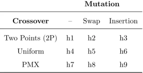
Table 1 presents the LLHs used in this work, which are composed by the operators mentioned in this subsection. We decided to include LLHs composed only by crossover operators (h1, h4 andh7), because this kind of operator is a distinguishing feature of evolutionary and genetic algorithms [40].
455
Table 1: Low-level heuristics composition
Mutation
Crossover – Swap Insertion
Two Points (2P) h1 h2 h3
Uniform h4 h5 h6
PMX h7 h8 h9
5.2. The measures r and t
As mentioned in the previous sections,r andt are updated in each genetic mating. Therefore, we implemented the credit assignment rules based on this fact. The update rules fortare straightforward: in each mating increment the tvalue for the LLHs not applied in that mating, and reset the counter to0for the applied one. Thus, thet value of a LLH is set in the interval[0..+∞]. On the other hand, for each LLH, itsrvalue is computed using the mating parents and the generated children as shown in Equation 6.
rh= 1 |P| · |C|· X p∈P X c∈C 1 ifc≺p 0 ifp≺c 0.5 otherwise (6)
whererh is the computedrvalue for the applied LLHh;P is the set of mating parents; pis a parent inP; C is the set of children generated in that mating; andcis a child inC. One comparison is done for each parent and child and the result of this comparison is summed. If a child dominates a parent (cp), then
460
and parent are non-dominated, then0.5is added. The sum result is normalized with 1/(|P| · |C|) to encompass algorithms that generate different numbers of children in each mating.
For instance, if two children generated by a LLH idominate both parents,
465
thenrh = 1. If the two parents dominate both children, then rh = 0. If both children are non-dominated in relation to their parents, then rh = 0.5. The higher the value ofrh, the better the LLHhperformed in that mating.
As far as we know, there are no reward measures for credit assignment that use solely the concept of Pareto dominance and only the individuals involved in
470
the mating. In some works, such as [28, 36], the reward is computed by compar-ing the generated solutions with the whole population uscompar-ing quality indicators for each generation or aftern(parameter) generations. One of the advantages of our measure is its straightforward implementation using explicitly the well-known Pareto dominance concept. In addition, it is potentially faster to execute,
475
because it uses only the mating solutions and some constant values, instead of complex population based indicators and several solutions. The minor drawback is the positive reward given to a LLH when using the worst possible individuals as parents, as it will usually generate children that dominate their parents.
The next subsections present how these measures are used by CF and MAB.
480
5.3. Choice Function Adaptation
The CF adaptation, proposed in this work, uses the measures t and r di-rectly. However, it still maintains the main features of this CF variation: an exploration and an exploitation factor. The adaptation proposed is a derivation of Equation 2, where thef1function was replaced by the direct value ofr, and
485
f2 was replaced by the direct value of t, while the weight parametersαand β were kept to balance the exploration and exploitation. Usually theαis set to1
andβto a very low decimal value (0.005or less), since therinterval is relatively small ([0,1]) when compared to thet interval ([0..+∞]).
5.4. Multi-Armed Bandit Adaptation
490
To adapt MAB we used the SlMAB [19] method. It is similar to the original equation presented in Subsection 2.2, changing only the rewardri,tand the time factort. In our implementation, the proposed r measure replaces the original instant rewardri,t, and the time factortreplaces(t−ti)in the equations.
In essence, the adapted MAB method is the same as the original [19], because
495
it differs only in the computing of the instant reward and the elapsed time. At the end of the evaluation, a LLH is chosen according to its value regarding Equation 3. The only parameter that needs to be tuned for this method isC, which balances the exploration and exploitation factors.
For both methods, CF and MAB, we used themax strategy selection. If CF
500
is being used as selection method, then the LLH with the maximum CF value is applied. If MAB is being used, then the LLH with the maximum MAB value is applied. If there is a tie in the CF/MAB value between two or more LLHs, then a random tied LLH is selected.
6. Empirical Evaluation
505
The empirical evaluation focuses on the results obtained by HITO when com-pared to two MOEAs. This section describes the research questions (RQs) that guided this evaluation, used systems, and how the algorithms were configured. Then, it presents the analyses and the results to answer the RQs.
6.1. Research Questions (RQs)
510
RQ1: How is the performance of HITO regarding the ITO problem? This question investigates if HITO can properly solve the considered problem when compared to two other conventional MOEAs: the well-known and widely used NSGA-II, and the state of the art MOEA/DD [34]. In addition, it investigates if HITO can overcome the results achieved by these conventional metaheuristics
515
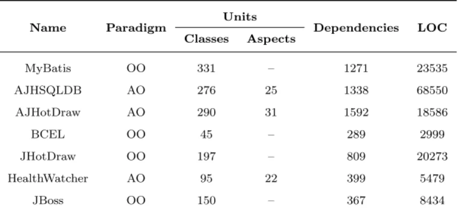
Table 2: Details of the systems used in the study
Name Paradigm Units Dependencies LOC
Classes Aspects MyBatis OO 331 – 1271 23535 AJHSQLDB AO 276 25 1338 68550 AJHotDraw AO 290 31 1592 18586 BCEL OO 45 – 289 2999 JHotDraw OO 197 – 809 20273 HealthWatcher AO 95 22 399 5479 JBoss OO 150 – 367 8434
RQ2: How is the performance of the selection methods CF and MAB? For answering this question, we analyzed the results of both selection methods in order to identify which one provides the best results.
RQ3: Which LLH is the most appropriate to this problem? To answer
520
this question, we analyzed the number of times each LLH (Subsection 5.1) was applied during the execution of HITO.
6.2. Systems Used in the Study
The real systems used in this work are detailed in Table 2. The first column presents the name of the systems. The second column presents the paradigm
525
of the system (OO or AO). The third and fourth columns present respectively how many classes (Cls.) and aspects (As.) (both considered units) exist in the system. The fifth column presents the number of dependencies between the units of the system. Finally, the sixth column presents how manyLines of Code
(LOC) the system has. Cells with a hyphen (-) represent none.
530
These are the same systems used in [4]. We chose to generate integration and test orders for these systems for a consistent comparison with this work. Moreover, some of these systems are AO, which inserts a bit of complexity to the problem, due to the increased number of dependencies between the units and to the different possible dependency scenarios.
6.3. Experiments Organization
In order to answer our questions we configured the following algorithms: i) MOEA/DD; ii) NSGA-II; iii) HITO-CF – algorithm that applies HITO with the CF selection method; iv) HITO-MAB – algorithm that applies HITO with the MAB selection method; and v) HITO-R – algorithm that applies HITO with
540
a random selection method. Each algorithm was executed 30 times for each system. The results were compared using the quality indicators hypervolume
and Inverted Generational Distance (IGD) [50]. We also computed the Kruskal-Wallis statistical tests (at 95% significance level) [15] and Vargha-Delaney’s  effect size [2] for the quality indicators’ results.
545
The hypervolume indicator computes the area (or volume when working with more than 2 objectives) of the objective space that a Pareto front dominates [50]. Its calculation is done using a reference point solution, usually the worst of all possible solutions. The advantage of hypervolume is that it takes into account both convergence and diversity. In addition, the software engineer is
550
able to determine if a Pareto front is better by comparing their hypervolume values. The greater the hypervolume value, the better the front is. The IGD indicator, in turn, calculates the distance of the true Pareto front (P Ftrue) to another front, thus the lower the IGD of a front, the better this front is. However, for our systems, the P Ftrue fronts are unknown. Due to this, we
555
generated an approximated P Ftrue for each system using the non-dominated solutions of the known Pareto fronts (P Fknown) found by the algorithms. A P Fknown front is composed by all the non-dominated solutions found in the 30 executions of an algorithm. Hence, each algorithm found aP Fknownfor a given system at the end of its 30 executions by joining the 30 resulting fronts. These
560
P Fknownfronts were later used to compose theP Ftrueapproximation by joining all non-dominated solutions, and to compute the IGD values for the algorithms. HITO was implemented using jMetal [17], an object-oriented framework for multi-objective evolutionary optimization. The conventional MOEAs and HITO were executed in all systems and with two sets of objective functions, according
565
Attributes (A) and Number of Operations (O)); and ii) a set of four objectives (A, O, Number of Distinct Return Types (R) and Number of Distinct Param-eters (P)). For all experiments we defined NSGA-II [14] as the MOEA used by HITO, since it is one of the common MOEAs used for solving this problem and
570
within the hyper-heuristics field for comparison [4, 28, 36, 47]. For executing the described algorithms, we used the chromosome representation and the con-straints adopted by the approach presented in [4], since this approach was used as a standard approach for the MOEA due to its good results.
The NSGA-II parameters were set according to [4], whereas the MOEA/DD
575
parameters were set according to [4, 34]. The parameters required by MAB and CF were set after an empirical tuning. This tuning was done to properly balance the different intervals between the credit assignment metricsr and t. The NSGA-II, MOEA/DD, HITO-CF, HITO-MAB and HITO-R parameters for this study are presented in Table 3. The CF weight parameters (αandβ),
580
and the MAB size of the sliding window (W) and scaling factor (C) are used to balance exploration and exploitation. Furthermore, MOEA/DD has three additional parameters when compared to NSGA-II: a penalty for the Penalty based Boundary Intersection (PBI) decomposition method, a neighborhood size (T), and a probability to select solutions from the neighborhood (δ).
585
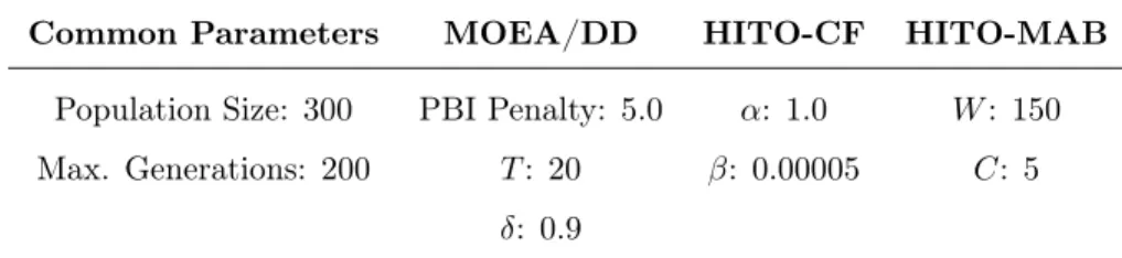
Table 3: Parameters
Common Parameters MOEA/DD HITO-CF HITO-MAB
Population Size: 300 PBI Penalty: 5.0 α: 1.0 W: 150
Max. Generations: 200 T: 20 β: 0.00005 C: 5
δ: 0.9
The mutation and crossover probabilities were set differently. For NSGA-II and MOEA/DD, we used a crossover probability of 95% and a mutation probability of 2%, as described in [4]. For CF, MAB and HITO-R, we did not use such probabilities because if a LLH is selected by HITO then
Figure 3: P Fknownfronts for MyBatis
Figure 4: P Fknownfronts for AJHSQLDB
its operators are mandatorily applied. Hence, the engineer does not need to
590
select the operators and configure their probability. This is one of the main advantages of HITO. Moreover, for MOEA/DD with 4 objectives, we had to set the population size to 364 in order to successfully generate weighting vectors.
6.4. Results
The obtained results are divided by number of objectives (2 and 4), but
595
they are discussed together. First, we analyzed the fronts generated by each algorithm. Figures 3-6 depictP Fknown fronts for 4 problems with 2 objectives. We presented only the plots that show visible differences between the fronts.
As seen in Figure 3 for MyBatis, NSGA-II, HITO-CF, and HITO-MAB ob-tained the best fronts with solutions overlapping each other. MOEA/DD was
600
able to find some solutions among the best ones, but some solutions found are dominated by the other algorithms. On the other hand, for AJHSQLDB in Figure 4, MOEA/DD obtained the majority of the non-dominated solu-tions, and HITO-CF just a few non-dominated solutions. For BCEL (Figure 5), only NSGA-II performed noticeable worse than the other algorithms.
Fi-605
nally, for AJHotDraw depicted in Figure 6, HITO-CF and HITO-MAB obtained all the non-dominated solutions, NSGA-II obtained intermediate solutions, and MOEA/DD and HITO-R obtained overlapping fronts with the worst solutions. Because the plots cannot reveal the best algorithm, the usage of quality indicators is necessary. Tables 4 and 5 show the average hypervolume found by
610
the algorithms for 2 and 4 objectives respectively. The average was computed using the 30 fronts found by each algorithm and for each system. For both tables,
Figure 6: P Fknownfronts for AJHotDraw
the first column shows the system, and the second, third, fourth, fifth and sixth columns show respectively the results obtained by MOEA/DD, NSGA-II, HITO-CF, HITO-MAB and HITO-R. Values highlighted in bold are the best values or
615
the values statistically equivalent to the best one using the Kruskal-Wallis test with 95% of significance. It is important to note that the Kruskal-Wallis test was performed using the 30 hypervolume values (one value for each independent run) of the resulting fronts of each algorithm, and not the average values alone.
Table 4: Hypervolume averages found for 2 objectives
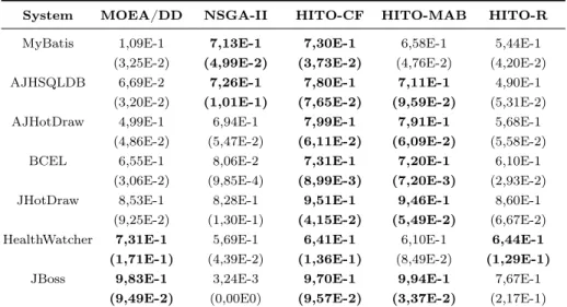
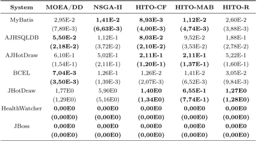
System MOEA/DD NSGA-II HITO-CF HITO-MAB HITO-R
MyBatis 6,81E-1 (4,41E-2) 7,65E-1 (3,96E-2) 8,00E-1 (2,71E-2) 7,83E-1 (3,06E-2) 6,88E-1 (2,37E-2) AJHSQLDB 7,41E-1 (7,94E-2) 5,86E-1 (1,12E-1) 6,90E-1 (6,76E-2) 6,45E-1 (1,06E-1) 4,11E-1 (6,86E-2) AJHotDraw 5,74E-1 (7,95E-2) 5,91E-1 (1,15E-1) 8,16E-1 (8,56E-2) 8,11E-1 (9,30E-2) 5,52E-1 (9,27E-2) BCEL 8,08E-1 (1,25E-2) 2,87E-1 (5,15E-3) 7,87E-1 (8,01E-3) 7,81E-1 (3,51E-2) 6,95E-1 (5,44E-2) JHotDraw 8,06E-1 (1,13E-1) 4,72E-1 (2,67E-1) 8,53E-1 (1,26E-1) 9,19E-1 (7,53E-2) 7,88E-1 (1,25E-1) HealthWatcher 8,17E-1 (5,45E-2) 8,52E-1 (2,61E-2) 8,65E-1 (2,57E-2) 8,80E-1 (4,36E-2) 8,78E-1 (4,14E-2) JBoss 9,50E-1 (1,40E-1) 5,38E-3 (0,00E0) 8,81E-1 (1,85E-1) 9,32E-1 (1,32E-1) 7,16E-1 (2,45E-1)
Because we normalized the objective values of all solutions into the interval
620
of[0..1], the worst possible value for the objectives is1(given that the problem is a minimization one). Hence, adding a small offset of 0.01, the reference point for the hypervolume calculation was set to (1.01,1.01) for 2 objectives and(1.01,1.01,1.01,1.01)for 4 objectives.
For every system, on both objective sets, HITO was able to outperform
625
NSGA-II by finding a greater hypervolume average. Only in four cases (Health-Watcher and MyBatis with 2 objectives, and MyBatis and AJHSQLDB with 4
Table 5: Hypervolume averages found for 4 objectives
System MOEA/DD NSGA-II HITO-CF HITO-MAB HITO-R
MyBatis 1,09E-1 (3,25E-2) 7,13E-1 (4,99E-2) 7,30E-1 (3,73E-2) 6,58E-1 (4,76E-2) 5,44E-1 (4,20E-2) AJHSQLDB 6,69E-2 (3,20E-2) 7,26E-1 (1,01E-1) 7,80E-1 (7,65E-2) 7,11E-1 (9,59E-2) 4,90E-1 (5,31E-2) AJHotDraw 4,99E-1 (4,86E-2) 6,94E-1 (5,47E-2) 7,99E-1 (6,11E-2) 7,91E-1 (6,09E-2) 5,68E-1 (5,58E-2) BCEL 6,55E-1 (3,06E-2) 8,06E-2 (9,85E-4) 7,31E-1 (8,99E-3) 7,20E-1 (7,20E-3) 6,10E-1 (2,93E-2) JHotDraw 8,53E-1 (9,25E-2) 8,28E-1 (1,30E-1) 9,51E-1 (4,15E-2) 9,46E-1 (5,49E-2) 8,60E-1 (6,67E-2) HealthWatcher 7,31E-1 (1,71E-1) 5,69E-1 (4,39E-2) 6,41E-1 (1,36E-1) 6,10E-1 (8,49E-2) 6,44E-1 (1,29E-1) JBoss 9,83E-1 (9,49E-2) 3,24E-3 (0,00E0) 9,70E-1 (9,57E-2) 9,94E-1 (3,37E-2) 7,67E-1 (2,17E-1)
objectives) NSGA-II yielded statistically equivalent results to the ones of HITO-CF and HITO-MAB. For MyBatis with 4 objectives, NSGA-II was statistically better than HITO-MAB, but yet HITO-CF outperformed it. MOEA/DD could
630
statistically outperform all the other algorithms only in BCEL with 2 objectives. Apart from that, it performed equally or worse than CF and/or HITO-MAB, sometimes even losing to NSGA-II. We expected a better performance from this state of the art algorithm, specially for 4 objectives where the benefits of decomposition could be better availed.
635
We also computed the IGD values for all 30 fronts obtained by the algorithms in each system. The reference front was generated joining all non-dominated solutions found in this experiment. These results are presented in Tables 6 and 7. MOEA/DD was only able to statistically outperform the other algorithms in BCEL with 2 objectives. Besides that, MOEA/DD presented mixed results
640
when compared to HITO-CF and HITO-MAB, always showing worse or equal results. For the biggest two systems with 4 objectives, NSGA-II obtained statis-tically equivalent results to HITO-CF. HITO-CF on the other hand presented the best overall results considering IGD. Except for BCEL with 2 objectives,
Table 6: IGD averages found for 2 objectives
System MOEA/DD NSGA-II HITO-CF HITO-MAB HITO-R
MyBatis 2,95E-2 (7,89E-3) 1,41E-2 (6,63E-3) 8,93E-3 (4,00E-3) 1,12E-2 (4,74E-3) 2,60E-2 (3,88E-3) AJHSQLDB 5,50E-2 (2,18E-2) 1,12E-1 (3,72E-2) 8,03E-2 (2,10E-2) 9,52E-2 (3,53E-2) 1,88E-1 (2,78E-2) AJHotDraw 6,10E-1 (1,54E-1) 5,02E-1 (2,11E-1) 2,11E-1 (1,20E-1) 2,11E-1 (1,37E-1) 5,22E-1 (1,60E-1) BCEL 7,04E-3 (3,50E-3) 1,26E-1 (1,39E-3) 1,26E-2 (2,07E-3) 1,41E-2 (6,52E-3) 3,05E-2 (9,84E-3) JHotDraw 1,77E0 (1,29E0) 5,90E0 (5,16E0) 1,40E0 (1,34E0) 6,55E-1 (7,74E-1) 1,27E0 (1,28E0) HealthWatcher 0,00E0 (0,00E0) 0,00E0 (0,00E0) 0,00E0 (0,00E0) 0,00E0 (0,00E0) 0,00E0 (0,00E0) JBoss 0,00E0 (0,00E0) 0,00E0 (0,00E0) 0,00E0 (0,00E0) 0,00E0 (0,00E0) 0,00E0 (0,00E0)
Table 7: IGD averages found for 4 objectives
System MOEA/DD NSGA-II HITO-CF HITO-MAB HITO-R
MyBatis 4,89E-2 (6,38E-3) 5,59E-3 (1,22E-3) 5,12E-3 (1,11E-3) 7,58E-3 (1,77E-3) 1,17E-2 (1,95E-3) AJHSQLDB 1,72E-1 (2,13E-2) 2,11E-2 (1,07E-2) 1,66E-2 (7,20E-3) 2,40E-2 (1,08E-2) 5,32E-2 (9,67E-3) AJHotDraw 8,99E-2 (1,82E-2) 4,48E-2 (8,90E-3) 3,22E-2 (8,90E-3) 3,27E-2 (8,89E-3) 8,49E-2 (1,89E-2) BCEL 1,90E-2 (2,79E-3) 1,28E-1 (1,80E-4) 9,63E-3 (2,60E-3) 9,03E-3 (9,15E-4) 2,11E-2 (2,52E-3) JHotDraw 2,36E-1 (1,14E-1) 2,05E-1 (1,35E-1) 9,91E-2 (3,79E-2) 9,50E-2 (4,31E-2) 1,74E-1 (5,48E-2) HealthWatcher 0,00E0 (0,00E0) 0,00E0 (0,00E0) 0,00E0 (0,00E0) 0,00E0 (0,00E0) 0,00E0 (0,00E0) JBoss 0,00E0 (0,00E0) 0,00E0 (0,00E0) 0,00E0 (0,00E0) 0,00E0 (0,00E0) 0,00E0 (0,00E0)
HITO-CF was always better or equal to the other algorithms. For both quality
645
indicators, HITO-R performed statistically worse or equal to HITO.
The HealthWatcher and JBoss instances appear to be the easiest to solve, since almost all algorithms yielded statistically equivalent results. Furthermore, when analyzing IGD, we observed that all algorithms were able to find the same
non-dominated solutions for both instances with both sets of objectives. They
650
are in fact two of the smallest system used in this study, hence the similarity of the results was expected.
We also calculated the Vargha-Delaney’s  effect size [2]. While Kruskal-Wallis calculates if there is statistical difference between groups of data, the effect size calculates the magnitude of this difference for each pair of groups
655
A/B of data. According to [2], the Aˆ value varies between [0,1], where 0.5
represents absolute no difference between the two groups, values below0.5 rep-resent that groupA loses to groupB, and values above 0.5 represent that B loses to groupA. Values in]0.44,0.56[represent negligible differences, values in
[0.56,0.64[and]0.36,0.44]represent small differences, values in[0.64,0.71[and
660
]0.29,0.44]represent medium differences, and values in [0.0,0.29]and[0.71,1.0]
represent large differences. A negligible magnitude usually does not yield statis-tical difference. The small and medium magnitudes represent small and medium differences between the values, and may or not yield statistical differences. Fi-nally, a large magnitude represents a significantly large difference that usually
665
can be seen in the numbers without a lot of effort.
Because we have computed the Aˆ value for each group comparison, in all systems, for both sets of objectives, and for both hypervolume and IGD values, we present the results in the format of boxplots with HITO-CF as group A. These boxplots are presented in Figures 7 to 10. The lower the values, the
670
worse the results of HITO-CF in comparison to the respective algorithm.
Figure 7: Hypervolume effect size for 2 objectives
Figure 8: Hypervolume effect size for 4 objectives
Figure 9: IGD effect size for 2 objectives
Figure 10: IGD effect size for 4 objectives
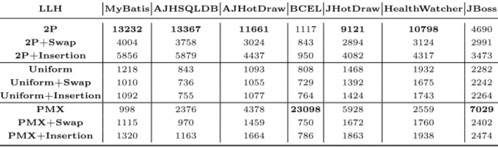
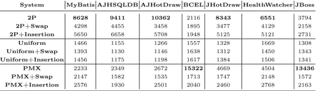
Table 8: Average number of low-level heuristic applications by HITO-CF with 2 objectives
LLH MyBatis AJHSQLDB AJHotDraw BCEL JHotDraw HealthWatcher JBoss 2P 13232 13367 11661 1117 9121 10798 4690 2P+Swap 4004 3758 3024 843 2894 3124 2991 2P+Insertion 5856 5879 4437 950 4082 4317 3473 Uniform 1218 843 1093 808 1468 1932 2282 Uniform+Swap 1010 736 1055 729 1392 1675 2242 Uniform+Insertion 1092 755 1077 764 1424 1743 2264 PMX 998 2376 4378 23098 5928 2559 7029 PMX+Swap 1115 970 1459 750 1672 1760 2402 PMX+Insertion 1320 1163 1664 786 1863 1938 2474
IGD comparisons. HITO-CF performed very similar to HITO-MAB in almost all cases. HITO-CF usually performed better than HITO-R and NSGA-II with large differences. Lastly, when comparing HITO-CF with MOEA/DD, we
ob-675
served more balanced results. Comparing the results for 2 objectives, HITO-CF showed effect size medians inside the small difference ranges, favorable in the hypervolume comparisons and unfavorable in the IGD comparison. However, for 4 objectives, MOEA/DD obtained worse results than HITO-CF, for both hypervolume and IGD, with medians in the large difference range.
680
We collected the average number of times each LLH was applied during the optimization. These averages were calculated using the 30 executions of each algorithm and are shown in Tables 8, 9, 10 and 11. The first two tables show the averages of HITO-CF and HITO-MAB with 2 objectives, and the last two the averages with 4 objectives. The greatest values are highlighted in bold.
685
We observed in all cases that the most applied LLHs are the ones composed only by crossover operators (h1 – 2P Crossover, h4 – Uniform Crossover and
h7 – PMX Crossover). Moreover, these three LLHs were applied more often than their respective LLHs with mutation operators. The most applied LLH is
h1 (2P Crossover), followed byh7 (PMX Crossover). In every scenario, h7 has
690
a greater number of applications for BCEL and JBoss. Additionally, h7 was applied more often in JHotDraw by HITO-MAB with 2 objectives. Apart from
Table 9: Average number of low-level heuristic applications by HITO-MAB with 2 objectives
System MyBatis AJHSQLDB AJHotDraw BCEL JHotDraw HealthWatcher JBoss
2P 8868 9954 9593 2882 7366 6254 3318 2P+Swap 4456 4264 2900 1571 2713 4129 1887 2P+Insertion 5954 6180 4297 1956 4373 5435 2582 Uniform 1419 1020 1209 1445 1266 1697 1163 Uniform+Swap 1219 1026 1166 1424 1288 1515 1244 Uniform+Insertion 1289 991 1223 1508 1402 1542 1206 PMX 2111 2837 5632 15418 7414 4241 14779 PMX+Swap 2057 1509 1623 1537 1653 2154 1509 PMX+Insertion 2473 2063 2204 2105 2372 2878 2159
Table 10: Average number of low-level heuristic applications by HITO-CF with 4 objectives
System MyBatis AJHSQLDB AJHotDraw BCEL JHotDraw HealthWatcher JBoss 2P 14430 14336 14796 389 13171 10241 4555 2P+Swap 4398 4096 3505 348 3044 3175 2991 2P+Insertion 6580 6198 6190 353 4861 4406 3503 Uniform 981 974 440 334 875 2178 2139 Uniform+Swap 706 786 390 313 768 1732 2095 Uniform+Insertion 933 887 419 316 819 1862 2116 PMX 499 1340 2346 27166 3701 2649 7821 PMX+Swap 619 579 809 308 1172 1733 2279 PMX+Insertion 699 650 952 318 1434 1869 2347
Table 11: Average number of low-level heuristic applications by HITO-MAB with 4 objectives
System MyBatis AJHSQLDB AJHotDraw BCEL JHotDraw HealthWatcher JBoss
2P 8628 9411 10362 2116 8343 6551 3794 2P+Swap 4298 4455 3458 1895 3477 4129 2158 2P+Insertion 5650 6658 5708 1948 5125 5121 2731 Uniform 1466 1155 1266 1557 1328 1669 1308 Uniform+Swap 1393 1130 1146 1638 1312 1450 1343 Uniform+Insertion 1456 1175 1198 1617 1384 1506 1341 PMX 2233 2349 2672 15322 4669 4504 13436 PMX+Swap 2147 1582 1535 1713 1747 2148 1572 PMX+Insertion 2576 1930 2501 2040 2460 2768 2163
these situations,h1 was always the most applied LLH.
The number of applications of each LLH is correlated to its overall perfor-mance during the optimization. If a given LLH was applied more than others,
695
then it means that this LLH constantly held a greater score throughout the pro-cess, and hence generated better children than others. Therefore, these numbers point out that, regardless of which selection method is being used, the PMX Crossover operator is the most suitable for BCEL and JHotDraw, and the Two Points Crossover operator is usually the most suitable for the remaining systems.
700
Furthermore, we observed that in most of the cases, the LLHs composed by Sim-ple Insertion Mutation were applied more often than the LLHs composed by the same crossover and Swap Mutation. It shows that Simple Insertion Mutation is overall the best mutation operator for this problem.
Using only crossover during the optimization generates the best children
705
in this kind of problem, whereas the usage of mutation operators can provide worse solutions in some cases. The reason behind this may be that, changing a lot the sequence of the genes is not always beneficial for permutation problems such as this one. This can be evidenced by the functionality of the operators. The crossover operators strictly use the sequence of the parents to generate the
710
children, whereas the mutation operators rely on randomness to insert diversity. Going even further, Simple Insertion Mutation is the best mutation operator because it changes the position of only one random gene, in contrast to Swap Mutation that changes the position of two random genes. In parallel, Two Points Crossover is the best crossover because it usually changes less the sequence of the
715
genes provided by the parents, whereas Uniform Crossover (the crossover least often applied) is the worst one because it performs the most drastic changes.
However, even though randomness is not always beneficial, the mutation operators should not simply be discarded, since they can provide diversity for the population in some moments of the search process. If the mutation operators
720
were useless, then the selection methods would have selected less often such LLHs. In some cases, the LLHs with mutation operators were applied more than the ones without these operators, which is understandable given the role that
the mutation plays in the evolution. Further investigations on the functionality of these operators in the hyper-heuristic field must be done in order to provide
725
a more comprehensive insight about their impact on the optimization process. Nevertheless, the real advantage here is that HITO can identify when it is preferable to apply each kind of operator and then can perform accordingly.
6.5. Answering the Research Questions
RQ1: How is the performance of HITO regarding the ITO problem?
730
As seen in the previous subsection, HITO (CF or MAB) was able to outperform or equal NSGA-II and HITO-R in all systems and for both sets of objectives re-garding the hypervolume and IGD indicators. When compared to MOEA/DD, in general, HITO was statistically better or equal, but MOEA/DD was the only algorithm able to outperform HITO with statistical difference in one system.
735
The effect size also supported these facts, since HITO usually outperformed NSGA-II, MOEA/DD and HITO-R with large or medium differences. Further-more, the IGD values show that HITO can also find the best P Fknown fronts for most systems, except BCEL where MOEA/DD stood out as the best al-gorithm. Taking these results into account, it is possible to assert that HITO
740
can properly solve this problem, and usually with better performance than an approach using only a conventional or state of the art MOEA. These positive results emphasize even more the applicability of hyper-heuristics in SBSE.
RQ2: How is the performance of CF and MAB?
Even though HITO-CF performed slightly better than HITO-MAB, it is not
745
possible to determine for sure if it is superior. The results of the Kruskal-Wallis test for the algorithms using both selection methods rarely showed statistical dif-ferences, and the effect size values usually presented negligible, small or medium magnitudes. We expected MAB to yield significant better results, since some of its equations focus on quickly identifying changes in the ranking of LLHs [19].
750
For future works, we intend to tweak the rewarding credit assignment equation (proposed in Subsection 5.2) for a better compatibility with MAB.
Overall, the best LLHs are composed only by crossover operators, specifically
h1 (Two Points Crossover) andh7 (PMX Crossover). The PMX operator is the
755
most suitable crossover for BCEL and JHotDraw, whereas Two Points Crossover is the best one for the other systems. Regarding the mutation operators, Simple Insertion Mutation performed better due to its small changes in the genes order.
6.6. Threats to Validity
Some systems used in the experimentation are small when compared to the
760
others, such as JBoss, HealthWatcher and JHotDraw. For instance, almost in all cases the results found by the algorithms for HealthWatcher are very similar, therefore, the Kruskal-Wallis test showed statistical equivalence between the results. The IGD indicator also showed that all algorithms found the same non-dominated solutions for HealthWatcher and JBoss. Thus, the results for these
765
systems cannot be generalized for larger systems.
The rewarding measure and the CF and MAB adaptations used by HITO may be accurate only for HITO using NSGA-II. For instance, if SPEA2 is used by HITO, then the time factor t of each LLH will scale quicker and the per-formance of HITO may be affected, since SPEA2 generates only one child per
770
mating in its implementation of the framework jMetal.
We used a fixed set of operators. Different operators can lead to differ-ent results. Therefore, we intend to evaluate other sets of operators in future work, such as newer operators, bigger sets of operators, different combinations of operators (e.g. no crossover, multiple mutation), and so on.
775
The MOEAs compared in this study were previously proposed and tested in continuous problems. This might be one explanation for their inferiority in comparison to HITO in the experimentation shown in this paper. Nevertheless, if the user is planning to arbitrarily choose and configure a MOEA for this problem, he/she should consider a hyper-heuristic instead, since it might be a
780
7. Concluding Remarks
In this study we introduced HITO, a hyper-heuristic for the ITO problem. HITO dynamically selects LLHs (combination of crossover and mutation op-erators) during the multi-objective evolutionary optimization. We proposed a
785
novel rewarding measure based on the Pareto dominance concept to assess the performance of each LLH. This metric is straightforward and uses only the par-ents and children involved in the mating. The reward is then used by selection methods, such as Choice Function (CF) and Multi-Armed Bandit (MAB), to select the best LLH at each mating. HITO was designed to encompass a set of
790
steps and to use inputs in order to allow the tester to flexibly personalize its execution. Therefore, the tester can provide his/her LLHs, MOEAs, software metrics to be used as fitness functions, selection methods and problem instances, according to his/her goals. However, the tester does not need to select the op-erators, nor to configure the algorithm parameters, because HITO makes such
795
decisions. This is an advantage of using hyper-heuristics.
HITO also presents other advantages. Even though we only used HITO to the ITO problem, it is a generic hyper-heuristic that can be applied for other software engineering problems and for any MOEA. For example, HITO can be used with SPEA2 [49] for solving problems such as prioritization and selection
800
of test cases, considering different objectives, such as coverage, size of test set, memory consumption, etc.
To evaluate HITO performance, we designed experiments with 2 and 4 objec-tives and used 7 real systems in an empirical evaluation, in both object-oriented and aspect-oriented contexts. We implemented the CF and MAB methods and
805
compared HITO with its random version, with a well-known MOEA (NSGA-II [14]), and with a state of the art MOEA (MOEA/DD [34]). HITO was able to outperform or statistically match NSGA-II and the random hyper-heuristic for all systems and sets of objectives. When compared to MOEA/DD, the results were also favorable in overall, but MOEA/DD was able to outperform HITO
810
performed similarly, but CF was slightly better. By analyzing the number of applications of each LLH, we observed that some crossover and mutation oper-ators are more suitable for the systems used, specifically Two Points Crossover and Simple Insertion Mutation.
815
Future works should to test the flexibility of HITO using other MOEAs and other problems to address its performance across the SBSE field. We also in-tend to increase the accuracy of the proposed rewarding measure by allowing a fine-grained evaluation of LLHs that hopefully will improve the results. Fur-thermore, HITO shall be evaluated using other selection methods and other
820
search operator. Moreover, other hyper-heuristic techniques can be used, such as on-line parameter tuning, metaheuristic selection and acceptance functions.
Instead of working solely on the search space of operators, hyper-heuristics can be employed to identify key characteristics of each system module. Later, these characteristics can be used to better guide the units ordering. Finally, we
825
will investigate why mutation operators were not so useful for this problem.
Acknowledgment
This work is supported by the Brazilian funding agencies CAPES and CNPq under the grants: 307762/2015-7 and 473899/2013-2.
References
830
[1] Ahandani, M. A., Baghmisheh, M. T. V., Zadeh, M. A. B., Ghaemi, S., 2012. Hybrid particle swarm optimization transplanted into a hyper-heuristic structure for solving examination timetabling problem. Swarm and Evolutionary Computation 7 (0), 21–34.
[2] András Vargha, H. D. D., 2000. A Critique and Improvement of the "CL"
835
Common Language Effect Size Statistics of McGraw and Wong. Journal of Educational and Behavioral Statistics 25 (2), 101–132.