Architectures and Algorithms for the Signal Processing of Advanced MIMO Radar Systems

(1)

UNIVERSITA’ DEGLI STUDI DI UDINE

Dipartimento Politecnico di Ingegneria e Architettura Corso di Dottorato in Ingegneria Industriale e dell’Informazione

Ciclo XXX

Tesi di Dottorato di Ricerca

Architectures and Algorithms for the

Signal Processing of Advanced MIMO

Radar Systems

Dottorando:

Alexander Rudolf Ganis

Relatore: Prof. Mirko Loghi Correlatori: Dipl.-Ing. Dr. VolkerZiegler (Airbus Group)

(2)

(3)

Abstract (Italiano)

Questa tesi si concentra sulla ricerca, lo sviluppo e l’implementazione di nuovi concetti, architetture, sistemi dimostrativi e algoritmi per l’elaborazione dei segnali in sistemi radar avanzati, basati su tecnologia Multiple Input Multiple Output (MIMO). Il con-cetto chiave `e quello di ottenere sistemi compatti, dalle elevate risoluzioni e in grado di eseguire un’elaborazione del segnale radar veloce, un beam-forming tri-dimensionale (3D) e quadri-dimensionale (4D) per la generazione di immagini radar e la stima delle informazioni dei bersagli, detti target. L’idea `e di ottenere una stima completa, che includa la distanza, l’Azimuth e l’elevazione (addizionalmente Doppler come quarta di-mensione) dai target nelle acquisizioni radar. La tecnologia radar indagata ha lo scopo di affrontare diverse applicazioni civili e militari, come la sorveglianza e la rilevazione di targets, sia a livello aereo che a terra, e la consapevolezza situazionale, sia nelle auto che nelle piattaforme di volo, dagli elicotteri, agli Unmanned Aerial Vehicels (UAV) e taxi volanti (air-taxis).

Le tematiche affrontante sono molte: Lo sviluppo di sistemi completi e di architetture digitali innovative, basate su tecnologia FPGA, ARM e software, per radar 3D MIMO, che operano in modalit`a Multiplexing Time Division Multiplexing (TDM) e Multiplexing Frequency Diversion (FDM), con segnali di tipo FMCW (Frequency Modulated Contin-uous Wave) e Orthogonal Frequency Division Multiplexing (OFDM), rispettivamente; Lo sviluppo di tecniche di elaborazione del segnale radar in tempo reale, algoritmi di beam-forming e di stima della direzione di arrivo, Direction-Of-Arrival (DOA), dei seg-nali radar, per il rilevamento dei target, con particolare attenzione a processi basati su trasformate di Fourier (FFT); Lo studio e l’implementazione di concetti di sistema avan-zati, parametrizzazione e simulazione di radar digitali di prossima generazione, capaci di operare in tempo reale (ad esempio basati su architetture OFDM). La progettazione e lo sviluppo di nuove forme d’onda ortogonali ad inviluppo costante per sistemi radar 3D di tipo OFDM MIMO, operanti in tempo reale.

Le attivit`a di ricerca di questa tesi sono state svolte presso la compagnia Airbus, con sede a Monaco di Baviera (Germania), nell’ambito di un programma di dottorato, svoltosi in maniera congiunta tra Airbus ed il Dipartimento Politecnico di Ingegneria e Architettura dell’Universit`a di Udine, con sede a Udine (Italia).

(4)

An investment in knowledge pays the best interest.

(5)

(6)

UNIVERSITY OF UDINE

Faculty of Engineering

Polytechnic Department of Engineering and Architecture In partial fulfillment of the requirements for the degree of

Doctor of Philosophy

Architectures and Algorithms for the

Signal Processing of Advanced MIMO

Radar Systems

Supervisors:

Prof. Mirko Loghi

Dipl.-Ing. Dr. Volker Ziegler (Airbus Group)

Author: Alexander Rudolf Ganis

(7)

Abstract

This thesis focuses on the research, development and implementation of novel concepts, architectures, demonstrator systems and algorithms for the signal processing of advanced Multiple Input Multiple Output (MIMO) radar systems. The key concept is to address compact systems, which have high resolutions and are able to perform a fast radar signal processing, three-dimensional (3D) and four-dimensional (4D) beamforming for radar image generation, and target estimation. The idea is to obtain a complete sensing of range, Azimuth and elevation (additionally Doppler as the fourth dimension) from the targets in the radar captures. The radar technology investigated, aims at addressing several civil and military applications, such as surveillance and detection of targets, both air and ground based, and situational awareness, both in cars and in flying platforms, from helicopters, to Unmanned Aerial Vehicles (UAV) and air-taxis.

Several major topics have been targeted. The development of complete systems and innovative FPGA, ARM and software based digital architectures for 3D imaging MIMO radars, which operate in both Time Division Multiplexing (TDM) and Frequency Divi-sion Multiplexing (FDM) modes, with Frequency Modulated Continuous Wave (FMCW) and Orthogonal Frequency Division Multiplexing (OFDM) signals, respectively. The de-velopment of real-time radar signal processing, beamforming and Direction-Of-Arrival (DOA) algorithms for target detection, with particular focus on FFT based, hardware implementable techniques. The study and implementation of advanced system concepts, parametrisation and simulation of next generation real-time digital radars (e.g. OFDM based). The design and development of novel constant envelope orthogonal waveforms for real-time 3D OFDM MIMO radar systems.

The MIMO architectures presented in this thesis are a collection of system concepts, de-sign and simulations, as well as complete radar demonstrators systems, with indoor and outdoor measurements. Several of the results shown, come in the form of radar images which have been captured in field-test, in different scenarios, which aid in showing the proper functionality of the systems.

The research activities for this thesis, have been carried out on the premises of Air-bus, based in Munich (Germany), as part of a Ph.D. candidate joint program between Airbus and the Polytechnic Department of Engineering and Architecture (Dipartimento Politecnico di Ingegneria e Architettura), of the University of Udine, based in Udine (Italy).

(8)

(9)

Acknowledgements

I would like to express my sincerest gratitude to my advisor Prof. Mirko Loghi for his continuous support throughout my Ph.D studies and related research, for his patience, motivation, and immense knowledge. His guidance helped me throughout my overall academic experience, dating back to my Master’s thesis accomplishments. I could not have imagined having a better advisor and mentor.

My deepest gratitude goes to my advisor within Airbus Group, Dr. Volker Ziegler, for providing me an opportunity to join his exceptional team, for his vast expertise, enthusi-asm, leadership and unrelenting support throughout my research. He has routinely gone beyond his duties to provide the team with the best projects and all means necessary to accomplish a great work, together with a uniquely great friendship spirit.

Profound gratitude goes to Ulrich Prechtel, Dr. Askold Meusling and Dr. Bernhard Schoenlinner, who have been truly dedicated mentors. I am particularly indebted to them for managing and actively developing the radar projects, for their constant support, inside and outside the lab, and for the countless insightful discussions, concept designs and overall results’ analysis throughout the whole Ph.D. experience.

I would like to thank my thesis committee: Prof. Fabrizio Berizzi and Prof. Fabrizio Argenti, for their insightful comments and feedback, which helped me achieve an even better overall thesis’ quality.

Special thanks go to my friend and team mate Enric Miralles for the stimulating dis-cussions, for the countless time spent together, for his great work, determination and capabilities, and overall moral support and fun we have had in the last four years. Sincere thanks go to my friend and team mate Avik Santra, who has always inspired me with his enthusiasm for signal processing and electronics and shared his amazingly wide and profound knowledge with expertise and strong passion, and to Thomas Multerer, Joffrey Lemercier, Pau Panareda-Busto, Peter Heise, Dushan Pamunuwa and all the other friends and colleagues I have met along the way, for all the great experiences and all the fun we had and we keep on having.

Finally, no words in the world could express the feelings and gratitude I have for my family, my parents Afra and Mario, my brother Maximilian, my sister Raffaella, for Farida, Paolo, Sofia, Kimberly and Diego. You are the best gift life has given me and represent the strongest motivation for all of my achievements. I love you all.

(10)

(11)

List of Figures

1.1 Principles of a radar device. A radio, i.e. electromagnetic, wave is

scat-tered back from a target. . . 2

1.2 Average atmospheric absorption of millimeter waves. . . 10

1.3 CAT accidents and serious incidents per phase of flight 2005-2015. . . 15

2.1 Maximum range . . . 24

2.2 Angle estimation using 2 RX antennas.. . . 27

2.3 Angle estimation using 4 RX antennas.. . . 29

2.4 Angle resolution improves with increasing number of RX antennas. . . 29

2.5 Angle estimation using 1 TX and 8 RX antennas.. . . 30

2.6 Angle estimation using 2 TX and 4 RX antennas.. . . 31

2.7 Two-Dimensional angle estimation using 4 TX and 4 RX antennas. . . 31

2.8 Radar three-dimensional coordinates system. . . 32

2.9 Basic overview of how an FMCW system operates. . . 33

2.10 Example of an FMCW signal, with central frequency of 77 GHz. The time domain and the spectrogram representations are shown in the top and bottom part of the image, respectively. [1] . . . 34

2.11 Example of a FMCW transmission scheme for a TDM MIMO array with 4 TX antennas. . . 39

3.1 Block diagram of the 3D Imaging FMCW 24x24 MIMO Radar Demon-strator. . . 44

3.2 Schematic representation of the MIMO antenna configuration with the physical array (left) showing the 24 TX antennas in blue, the 24 RX antennas in red and the resulting virtual array (right). . . 45

3.3 The graph illustrates a simulation of virtual array pattern with the de-signed maximum beamsteering of ✓0 = 25◦ in red, the single element in blue and the resultant multiplication of both in black. The patterns are displayed in polar (subfigure A) and cartesian (subfigure B) coordinates. . 46

3.4 Representation of the used layer stack-up. . . 47

3.5 Photograph of the complete TX panel (left) and the corresponding block diagram (right).. . . 48

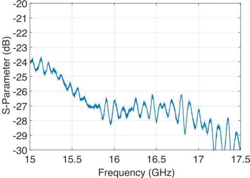
3.6 S-Parameters of the transmission from antenna 1 and 12. The effects of the coupler are compensated. . . 48

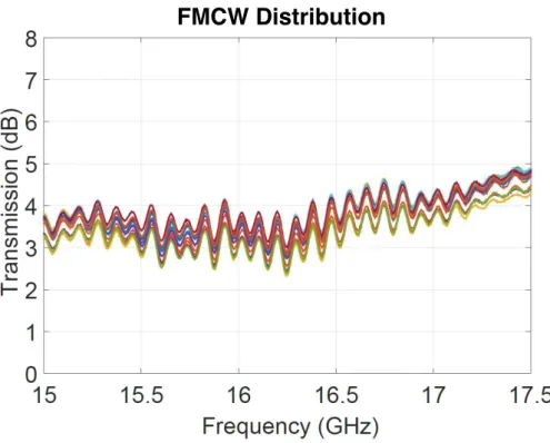
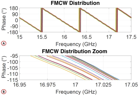
3.7 Photograph of the FMCW signal distribution board with its 16 output ports. . . 49

3.8 Amplitude comparison between all channels of the FMCW distribution board. . . 50 3.9 Phase comparison between all channels of the FMCW distribution board. 51

(16)

List of Figures xvi 3.10 Photograph of the receiver board, on the left, and corresponding block

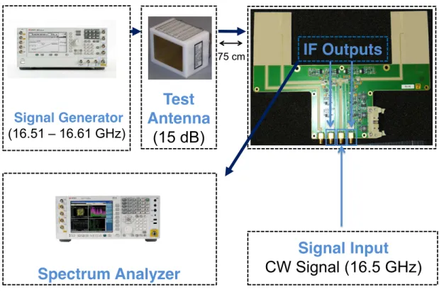
diagram, on the right. . . 52 3.11 Measurement setup for testing the performance of the receiver board and

the equalizer. . . 53 3.12 Screenshot of the measurement of the IF output performance of the RX

board, captured by a spectrum analyzer. . . 54 3.13 Measured maximum coupling between one TX and one RX antenna. The

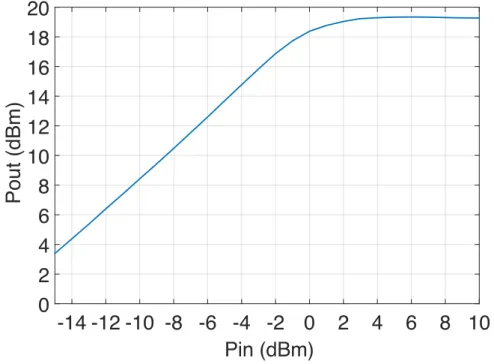
chosen elements were adjacent, with a distance (d) of 15 mm. . . 55 3.14 Measured input power versus output power in the transmitter board. The

measurement was performed from the input to the coupler C1 before the antenna. The effects of the coupler are compensated. . . 56 3.15 Photographs of the stacked TX, RX and FMCW signal distribution

pan-els. The left image shows the complete RF front-end unit. The right image is a section view of its structure.. . . 56 3.16 Photographs of the complete MIMO radar system. In the upper left

image, the integrated RF front-end and digital system is presented. On the lower left and right images, a front view of the antenna array is shown. 57 3.17 3D illustration of the complete digital unit with the 3 FMC-FPGA boards,

the PowerPC and the DDS and PLL board. . . 58 3.18 Schematic overview of the firmware implemented for the 4DSP FMC108

FMC modules. . . 58 3.19 Picture of the MIMO radar control graphic human machine interface (HMI). 59 3.20 Radar digital signal processing software architecture. . . 60 3.21 Range compression through FFT view of the received signal from one of

the virtual elements. . . 62 3.22 Illustration of the timings for a complete MIMO cycle: transmission for

all 24 TX elements, data acquisition, transfer and radar image processing. 63 3.23 The MIMO radar test field with two corner reflectors at a range of 60 m

with nominal radar cross section (RCS) of 36m2_. _{. . . 64} 3.24 Range-Azimuth section view of the 3D MIMO radar image capture from

the radar setup scenario with two reflectors at a distance of 60 m. . . 65 3.25 Range-Elevation section view of the 3D MIMO radar image capture from

the radar setup scenario with two reflectors at a distance of 60 m. . . 66 3.26 Range-Azimuth section view of the 3D radar image capture, with DBF

and MIMO processing, with the two corner reflectors placed at the same azimuth angle of around 0◦ _{and 1.5 m apart.} _{. . . 67} 3.27 Range-Azimuth section view of the 3D radar image capture, with DBF

and MIMO processing, with the two corner reflectors placed at the same azimuth angle of around 0◦ _{and 0.5 m apart.} _{. . . 67} 3.28 FFT view of the 3D radar image capture, cut across ranges, with DBF

and MIMO processing, with the two corner reflectors placed at the same azimuth angle of around 0◦ and 0.5 m apart. . . 68 3.29 Range-Azimuth section view of the 3D radar image capture, with

conven-tional DBF and no MIMO processing. The corner reflectors are placed at an identical range cell. The two targets are not uniquely identifiable. . . . 68 3.30 dB - Angular section view of the 3D radar image capture, with

conven-tional DBF and no MIMO processing. The corner reflectors are placed at an identical range cell. The two targets are not uniquely identifiable. . . . 69

(17)

List of Figures xvii 3.31 Range-Azimuth section view of the 3D radar image capture, with DBF

and MIMO processing. The corner reflectors are placed at an identical range cell. The two targets are uniquely identifiable. . . 69 3.32 dB - Angular section view of the 3D radar image capture, with DBF and

MIMO processing. The corner reflectors are placed at an identical range cell. The two targets are uniquely identifiable.. . . 70 3.33 Procedure for the measurement inside the anechoic chamber. A target is

placed at a distance of 24.5 meters and in front of the radar at 0◦ _{of both} Azimuth and elevation angles. . . 71 3.34 Picture of the anechoic chamber for the measurement of the angular

res-olution. The target is placed at a distance of 24.5 meters. . . 72 3.35 Picture of the anechoic chamber for the measurement of the angular

res-olution. View from the position of the target, towards the radar position. 72 3.36 dB - Azimuth, angular section view of the 3D radar image capture of the

target at 24.5 m, in the anechoic chamber. . . 73 3.37 dB - Elevation, angular section view of the 3D radar image capture of the

target at 24.5 m, in the anechoic chamber. . . 74 3.38 FFT view of the 3D radar image capture, cut across ranges, for the target

at 24.5 m, in the anechoic chamber. . . 75 3.39 Azimuth-range section view of the 3D radar image capture of the target

at 24.5 m, in the anechoic chamber. . . 75 3.40 Elevation-range section view of the 3D radar image capture of the target

at 24.5 m, in the anechoic chamber. . . 76 3.41 The MIMO radar test field with four corner reflectors at ranges of 14 m,

18.5 m, 22 m and 24 m with nominal radar cross section of 36m2_. _{. . . . 78} 3.42 Azimuth-range section view of the 3D radar image capture of four targets

at 14 m, 18.5 m, 22 m and 24 m, spaced both in Azimuth and in elevation. 78 3.43 Elevation-range section view of the 3D radar image capture of four targets

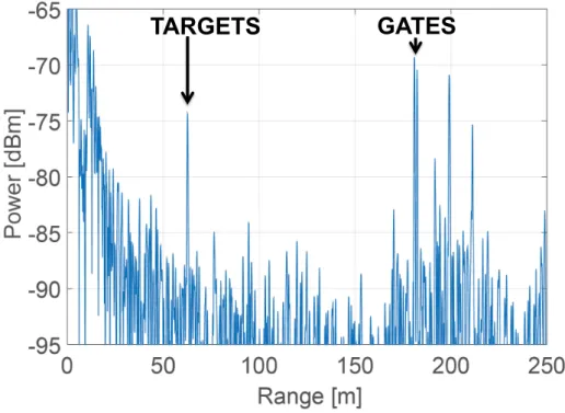
at 14 m, 18.5 m, 22 m and 24 m, spaced both in Azimuth and in elevation. 79 3.44 FFT view of the 3D radar image capture, cut across ranges, of four targets

at 14 m, 18.5 m, 22 m and 24 m. . . 79 3.45 dB - Azimuth, angular section view of the 3D radar image capture of the

target at 14 m and ✓= 0◦_._{. . . 80} 3.46 dB - Azimuth, angular section view of the 3D radar image capture of the

target at 18.5 m and✓=−4◦_. _{. . . 81} 3.47 dB - Azimuth, angular section view of the 3D radar image capture of the

target at 22 m and ✓=−9◦_._{. . . 82} 3.48 dB - Azimuth, angular section view of the 3D radar image capture of the

target at 24 m and ✓= 8◦_._{. . . 83} 3.49 dB - elevation, angular section view of the 3D radar image capture of the

target at 14 m and φ=−3◦_._{. . . 84} 3.50 dB - elevation, angular section view of the 3D radar image capture of the

target at 18.5 m andφ=−3◦_._{. . . 85} 3.51 dB - elevation, angular section view of the 3D radar image capture of the

target at 22 m and φ=−1◦_._{. . . 85} 3.52 dB - elevation, angular section view of the 3D radar image capture of the

(18)

List of Figures xviii 3.53 The MIMO radar test field with one corner reflector at ranges of 315 m,

with nominal radar cross section of 36 m2. . . 86 3.54 Range-Azimuth section view of the 3D radar image capture, with 1 corner

reflector visible at 315 meters. . . 87 4.1 Visualization of a rectangular MIMO array with unoccupied space in the

center (left) and a camera (right). . . 92 4.2 Block diagram of the 3D imaging FMCW 16x16 MIMO radar

demonstra-tor. The main components are the antenna board, the digital board, the DDS board, the receiver, the laptop and the camera. . . 93 4.3 Component level block diagrams of the antenna board and the receiver

with schematic of the switch chains. . . 94 4.4 Picture of the 3D printed housing with antenna board and camera mounted

in the middle. The markers show where the TX and RX antennas, and the camera are placed. . . 94 4.5 Picture of the back of the RF front-end antenna board, with 16 TX and

16 RX antenna elements, switch matrixes and a 3-way wilkinson divider. . 95 4.6 Picture of the receiver board, with the 16 channel paths to intermediate

frequency (IF), with the FMCW signal distribution for de-ramping, the RX inputs, the mixers and the filters. . . 96 4.7 Frequency response of the receiver board. . . 96 4.8 Pictures of the digital board, based on a ZYNQ SoC, with ARM and

FPGA, and integrated ADCs. . . 97 4.9 Schematic view of the main components and functionalities of the digital

board. . . 98 4.10 Schematic view of the digital architecture for the radar processing, from

the sampling of the radar signals, to the radar image generation. . . 99 4.11 Picture from the Xilinx Vivado tool, depicting the main blocks

imple-mented in the VHDL firmware for the radar processing. . . 100 4.12 Schematic view of the VHDL firmware for the radar processing,

imple-mented in the Xilinx Vivado tool.. . . 101 4.13 Radar digital signal processing software architecture, based on the

3D-FFT beam-forming. . . 104 4.14 Schematic representation of the MIMO antenna configuration with the

physical array (left) showing the 16 TX antennas in blue, the 16 RX antennas in red and the resulting virtual array (right). A unit in the graph is equivalent to dx

2 and

dy

2 respectively. . . 106 4.15 Exemplary timing of a MIMO cycle. . . 110 4.16 Picture of the anechoic chamber for the measurement of the angular

res-olution. The target is placed at a distance of 23.5 meters. . . 111 4.17 Azimuth profile, angular section view of the 3D radar image capture of

the target at 23.5 m, in the anechoic chamber. . . 111 4.18 Elevation profile, angular section view of the 3D radar image capture of

the target at 23.5 m, in the anechoic chamber. . . 112 4.19 Superposition of Azimuth and elevation profiles, angular section views

of the 3D radar image capture of the target at 23.5 m, in the anechoic chamber.. . . 112 4.20 FFT across range plot, section view of the 3D radar image capture of the

(19)

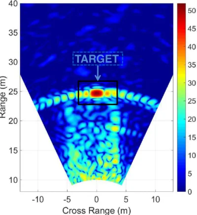
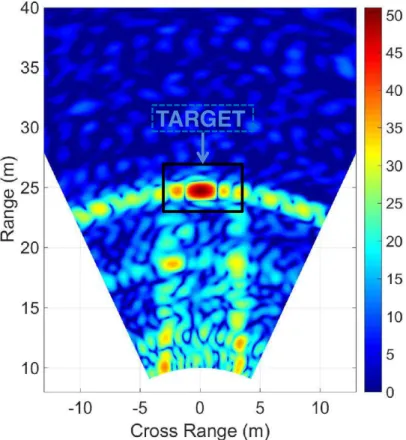
List of Figures xix 4.21 Range profile, zoom in of the plot in Fig. 4.20. . . 114 4.22 Azimuth-range section view of the 3D radar image capture of the target

at 23.5 m, in the anechoic chamber. . . 115 4.23 Range-elevation section view of the 3D radar image capture of the target

at 23.5 m, in the anechoic chamber. . . 115 4.24 Azimuth-elevation section view of the 3D radar image capture of the

target at 23.5 m, in the anechoic chamber. . . 116 4.25 Normalized dependence of the received power in the elevation direction

with the angle due to the antenna element pattern. . . 117 4.26 Normalized dependence of the received power in the azimuth direction

with the angle due to the antenna element pattern. . . 118 4.27 Azimuth-elevation section view of the 3D radar image capture of the

target at 197 m. . . 119 4.28 Range-elevation section view of the 3D radar image capture of the target

at 197 m. . . 119 4.29 Image of the scene with three corner reflectors at 18 m, 28 m and 22 m,

and a UAV at 8 m, marked with white circles.. . . 120 4.30 Azimuth-elevation section view of the 3D radar image capture of the 3

targets at 18 m, 28 m and 22 m, and the UAV at 8 m. . . 121 4.31 Range-elevation section view of the 3D radar image capture of the 3

tar-gets at 18 m, 28 m and 22 m, and the UAV at 8 m.. . . 122 4.32 3D reconstruction of the scene with radar data. The three targets are

spaced in range and have different positions in azimuth and elevation. . . 123 4.33 Camera and radar image overlaid. The color and the level of opaqueness

is proportional to the amplitude of the reflection. The targets’ ranges are displayed in boxes with different colors. The field of view is limited by the camera. . . 124 4.34 Imaging scenario captured with in-built camera, on the left (A).

Range-elevation section view of the 3D radar image capture, cut at ✓ = −21◦_, on the right (B). The left tree, circled in red, is the main object in the scene. . . 125 4.35 Imaging scenario captured with in-built camera, on the left (A).

Range-elevation section view of the 3D radar image capture, cut at ✓ = +10◦_, on the right (B). The right tree, circled in red, is the main object in the scene. . . 125 4.36 Imaging scenario captured with in-built camera, on the left (A).

Range-elevation section view of the 3D radar image capture, cut at ✓ = 0◦, on the right (B). The two hills represent the main objects in the scene. . . . 126 4.37 Images captured with in-built camera, on the left, in (A), (C) and (E).

The scene presents a UAV flying from a distance of 22 m to a distance of 30 m. Corresponding Azimuth-range section views of the 3D radar image captures, cut atφ= 0◦, are shown on the right, in (B), (D) and (F). . . . 129 4.38 Images captured with in-built camera, on the left, in (A), (C) and (E).

The scene presents a UAV flying from a distance of 31 m to a distance of 35 m. Corresponding Azimuth-range section views of the 3D radar image captures, cut atφ= 0◦_{, are shown on the right, in (B), (D) and (F).} _{. . . 130}

(20)

List of Figures xx 4.39 Images captured with in-built camera, on the left, in (A), (C) and (E). The

scene presents a person walking from a distance of 55.6 m and Azimuth angle of ✓ = 11.6◦_{, to a distance of 46 m and Azimuth angle of} _✓ ₌ 17.9◦_{. Corresponding Azimuth-range section views of the 3D radar image} captures, cut atφ= 0◦_{, are shown on the right, in (B), (D) and (F).} _{. . . 132} 4.40 Images captured with in-built camera, on the left, in (A), (C) and (E). The

scene presents a person walking from a distance of 40.9 m and Azimuth angle of ✓ = 22.3◦_{, to a distance of 24.9 m and Azimuth angle of} _✓ ₌ 27.5◦_{. Corresponding Azimuth-range section views of the 3D radar image} captures, cut atφ= 0◦_{, are shown on the right, in (B), (D) and (F).} _{. . . 133} 4.41 Block diagram of the MIMO radar and jamming system. . . 135 4.42 Prototype of the jamming unit consisting of a servo controller, a 2-axis

gimbal and a directional antenna. . . 136 4.43 The use of a directional antenna allows to jam at longer distances also

when the remote control (RC) is close by. In the given scenario a maxi-mum range of 250 m is reached with a 16 dBi antenna. . . 136 4.44 Measurement setup consisting of the 3D MIMO radar, jammer and

pro-cessing unit with a drone hovering in the foreground, on the left (A). On the right (B), an Azimuth-range view of a drone approaching at 60 m, as captured by the MIMO radar, is shown. The white crosses represent the tracked target. . . 137 4.45 Screenshot of the drone control GUI while jammer is active. Control link

is lost and can only be retaken by deactivating the jammer and recon-necting to the WiFi. . . 138 5.1 Generation of OFDM carriers. The basis is a rect-function with symbol

duration Ts, displayed on the left. The spectrum of the rect-function,

which is the sinc-function, is displayed on the right.. . . 143 5.2 Example of OFDM symbol composed of four orthogonal subcarriers with

spacing ∆f . . . 144 6.1 Top level view of the complete system architecture. . . 153 6.2 Time domain view of an LFM signal. The real and imaginary part are

represented in the upper and lower part of the image, respectively. . . 154 6.3 Schematic representation of the orthogonal waveforms generation

archi-tecture. . . 155 6.4 Cross Ambiguity Function of Golay Complementary Pair based LFM

waveforms. . . 157 6.5 Cross Ambiguity Function of Golay Complementary Pair based LFM

waveforms, across zero Delay, on the left in A, and across zero Doppler, on the right in B. . . 158 6.6 Cross Ambiguity Function of Zadoff Chu sequence based LFM waveforms. 159 6.7 Cross Ambiguity Function of Zadoff Chu sequence based LFM waveforms,

across zero Delay, on the left in A, and across zero Doppler, on the right in B. . . 159 6.8 Cross Ambiguity Function of Walsh-Hadamard based LFM waveforms. . . 160 6.9 Cross Ambiguity Function of Walsh-Hadamard based LFM waveforms,

across zero Delay, on the left in A, and across zero Doppler, on the right in B. . . 160

(21)

List of Figures xxi 6.10 Cross Ambiguity Function of Space-Time Code based LFM waveforms.. . 162 6.11 Cross Ambiguity Function of Space-Time Code based LFM waveforms,

across zero Delay, on the left in A, and across zero Doppler, on the right in B. . . 162 6.12 Cross Ambiguity Function of DFT based LFM waveforms. . . 163 6.13 Cross Ambiguity Function of DFT code based LFM waveforms, across

zero Delay, on the left in A, and across zero Doppler, on the right in B. . 163 6.14 Cross Ambiguity Function of Costas sequence based LFM waveforms. . . 164 6.15 Cross Ambiguity Function of Costas sequence based LFM waveforms,

across zero Delay, on the left in A, and across zero Doppler, on the right in B. . . 165 6.16 Woodward Ambiguity Function of the proposed LFM based waveforms. . 166 6.17 Receiver processing architecture. . . 167 6.18 4D-FFT beamforming architecture. . . 168 6.19 2x16 antenna array. The RX array configuration is shown in blue, while

the TX array in red. . . 169 6.20 Virtual antenna array. It is the results of the convolution between the

TX and RX arrays. . . 170 6.21 Range-Doppler map of Golay Complementary Sequence at -10 dB SINR. . 173 6.22 Range-Doppler map of Golay Complementary Sequence at 10 dB SINR. . 173 6.23 Range-Doppler map of Zadoff-Chu Sequence at -10 dB SINR. . . 174 6.24 Range-Doppler map of Zadoff-Chu Sequence at 10 dB SINR. . . 174 6.25 Range-Doppler map of Space-Time based LFM waveforms at -10 dB SINR.175 6.26 Range-Doppler map of Space-Time based LFM waveforms at 10 dB SINR.176 6.27 Range-Doppler map of Walsh-Hadamard based LFM waveforms at -10

dB SINR. . . 177 6.28 Range-Doppler map of Walsh-Hadamard based LFM waveforms at 10 dB

SINR. . . 178 6.29 Range-Doppler map of DFT based LFM waveforms at -10 dB SINR. . . . 179 6.30 Range-Doppler map of DFT based LFM waveforms at 10 dB SINR. . . . 179 6.31 Range-Doppler map of Costas sequence at -10 dB SINR. . . 180 6.32 Range-Doppler map of Costas sequence at 10 dB SINR. . . 180 6.33 Range-Azimuth plot of Golay Complementary pair waveform at -10 dB

SINR. . . 181 6.34 Range-Azimuth plot of Golay Complementary pair waveform at 10 dB

SINR. . . 181 6.35 Range-Azimuth plot of Zadoff Chu sequence at -10 dB SINR. . . 182 6.36 Range-Azimuth plot of Zadoff Chu sequence at 10 dB SINR. . . 182 6.37 Range-Azimuth plot of Space-Time based LFM waveform at -10 dB SINR.183 6.38 Range-Azimuth plot of Space-Time based LFM waveform at 10 dB SINR. 183 6.39 Range-Azimuth plot of Walsh-Hadamard based LFM waveform at -10 dB

SINR. . . 184 6.40 Range-Azimuth plot of Walsh-Hadamard based LFM waveform at 10 dB

SINR. . . 184 6.41 Range-Azimuth plot of DFT based LFM waveform at -10 dB SINR. . . . 185 6.42 Range-Azimuth plot of DFT based LFM waveform at 10 dB SINR. . . 185 6.43 Range-Azimuth plot of Costas sequence at -10 dB SINR.. . . 186 6.44 Range-Azimuth plot of Costas sequence at 10 dB SINR. . . 186

(22)

List of Figures xxii 6.45 Range-elevation plots of all of the proposed LFM based OFDM radar

waveforms at -10 dB SINR. . . 187 6.46 3D radar image of Costas sequence based LFM waveform at 10 dB SINR. 188 7.1 OFDM MIMO radar top-level block diagram . . . 190 7.2 Front-view (left) and back-view (right) of the OFDM MIMO radar. . . 190 7.3 Schematic view of the digital architecture for the OFDM radar processing,

from the sampling of the radar signals, to the radar image generation. . . 192 7.4 Picture from the Xilinx Vivado tool, depicting the main blocks

imple-mented in the VHDL firmware for the radar processing. . . 193 7.5 Schematic view of the VHDL firmware for the radar processing,

imple-mented in the Xilinx Vivado tool.. . . 194 7.6 Walsh Hadamard coded LFM based OFDM radar waveform: chirp

sig-nal’s time-domain view in the upper left, magnitude of the FFT view in the upper right, double and single sided power spectral density, in the lower left and lower right, respectively. . . 197 7.7 Top-level view of the implemented System Generator based architecture,

for the generation of the OFDM radar waveform’s values, to be stored and sent to the DACs. . . 199 7.8 Inside view of theSubsystem T X block of the implemented System

Gen-erator based architecture from Fig. 7.7. The ROM memories which store the values of the OFDM radar waveform are visible on the right side of the image. . . 200 7.9 Spectrum of the LFM based OFDM radar waveform sent from antenna

TX1, captured with a spectrum analyzer. . . 202 7.10 Zoom in of the spectrum of the LFM based OFDM radar waveform sent

from antenna TX1, shown in Fig. 7.9. . . 203 7.11 2x16 antenna array. The RX array configuration is shown in blue, while

the TX array in red. . . 206 7.12 Virtual antenna array. It is the results of the convolution between the

TX and RX arrays. . . 207 7.13 Scenario captured by the radar, with a corner cube centrally positioned

at 25 m and wire fence at 50 m.. . . 208 7.14 Azimuth-range view of the scene shown in Fig. 7.13. . . 208 7.15 Azimuth-elevation view of the scene shown in Fig. 7.13. . . 209

(23)

List of Tables

1.1 Radar Frequencies, Bands, Wavelength and Applications . . . 9 3.1 Targets’ Parameters for the Four Target Scenario . . . 76 3.2 Structure and Performance Comparison of Different Imaging Radars. . . . 81 4.1 FFT’s Original and Reordered, Indexes and Corresponding DOA Angles,

for the Azimuth Angles. . . 108 4.2 FFT’s Original and Reordered, Indexes and Corresponding DOA Angles,

for the Elevation Angles.. . . 108 5.1 Model Parameters Summary. . . 149 6.1 Cross Ambiguity Function Parameter Summary . . . 166 6.2 Target Parameters Summary . . . 172 7.1 3D OFDM MIMO Radar’s Parameters Summary . . . 196

(24)

(25)

Abbreviations

2D 2-Two Dimensional 3D 3-Three Dimensional 4D 4-Four Dimensional A/C Air - Craft

ADC Analog to Digital Converter AF Ambiguity Function

AM AmplitudeModulated ARM AdvancedRISC Machines ASM AlgorithmicStateMachine AWGN Additive White GaussianNoise CFAR CostantFalse AlarmRate COTS CommercialOff The Shelf CP CyclicPrefix

CPLD ComplexProgrammableLogicDevice CW ContinuosWaveform

DAC Digital to Analog Converter DBF Digital to BeamForming DC Direct Current

DDS Direct Digital Synthesiser DDR Double Data Rate

DFT DiscreteFourier Transform DMA Direct MemoryAccess DOA Direction Of Arrival DSP Digital Signal Processing

FDM FrequencyDivisionMultiplexing xxv

(26)

Abbreviations xxvi FDM FrequencyDivisionMultiple Access

FIFO FirstIn FirstOut FFT FastFourier Transform FM FrequencyModulated FM FPGA Mezzanine Card

FMCW FrequencyModulated Continuos Waveform FOV Field Of View

FPGA Field ProgrammableGateArray FSM FiniteStateMachine

FSPL FreeSpacePathLoss FTP File TransferProtocol GPS Global PositioningSystem GSPS GigaSamplesPerSecond GUI Graphical User Interface

HDL HardwareDescriptionLanguage HMI HumanMachineInterface ICI InterCarrier Interference

IDFT Inverse DiscreteFourierTransform

IEEE Institute of Electrical and Electronic Engineers IF Intermediate Frequency

IFFT Inverse FastFourierTransform IFT Inverse FourierTransform

ISAR Inverse Synthetic Aperture Array ISI InterSymbolInterference

ITU InternationalTelecommunicationUnion LFM Linear FrequencyModulated

LNA Low Noise Amplifier LO LocalOscillator LOS Line Of Sight LSB Least SignificantBit MEX Matlab EXecutable

MIMO Multiple InputMultiple Output MPC Multi PathComponent

(27)

Abbreviations xxvii MSB MostSignificantBit

MSPS MegaSamples PerSecond MTI Moving Target Indicator

NLFM NonLinear FrequencyModulated NLOS NonLineOf Sight

OFDM Orthogonal FrequencyDivision Multiplexing PAPR Peak toAaveragePowerRatio

PCB Printed Circuit Board PLL PhaseLockedLoop

PRF Pulse RepetitionFrequency RCS RadarCross Section

RF Radio Frequency

RADAR Radio Detection And Ranging RAM Random AccessMemory ROM ReadOnly Memory

RSPA Resonant Slot PatchAntenna

RX Receiver

SAR SyntheticAperture Array SDR SoftwareDefinedRadio

SFP SmallForm-factorPluggable (Transceiver) SFTP SSHFile TransferProtocol

SIMO SingleInputMultipleOutput SNR Signal toNoise Ratio

SINR Signal toInterference plusNoiseRatio SoC SystemonChip

SPI SerialPeriferalInterface SSH SecureSHell

STBC SpaceTime BlockCode SWAP SizeWeigth andPower TDL Tapped Delay Line

TDM Time Division Multiplexing TSA TaperedSlotAntenna

(28)

Abbreviations xxviii UAV UnmannedAerialVehicle

UART UniversalAsynchronous ReceiverTransmitter UDP UserDatagramProtocol

USB UniversalSerialBus

VHDL VHSICHardwareDescriptionLanguage VHSIC Very High Speed IntegratedCircuits VTOL VerticalTakeOff and Landing

(29)

Symbols

h(t, ⌧) Impulse response of the time-varying channel

NAZI Number of Elements Along the Azimuth’s Axis

NELE Number of Elements Along the Elevations’s Axis

NRAN GE Number of Elements Along the Range’s Axis

NT X Number of Transmit Antenna Elements

NRX Number of Receive Antenna Elements

Nvirtual Number of Virtual Antenna Elements

Nmeasures Number of Measurements

Nsamples Number of Samples

N Number of Subcarriers in an OFDM Symbol

M Number of Symbols in an OFDM Frame

NF RAM E Number of Samples in an OFDM Frame

Rn n-th Receive Antenna

Tn n-th Transmit Antenna

x(t) Transmitted signal

y(t) Received signal

B Signal’s Bandwidth Hz

Bef f Effective’s Signal’s Bandwidth Hz

c0 Speed of Light c= 2.997 924 58⇥108 ms−s

fC Carrier’s Frequency Hz

fD Doppler Shift Hz

fDmax Maximum Doppler Shift Hz

fs Sampling’s Frequency Hz

G Antenna Gain dBi

(30)

Symbols xxx

R Range m

Rmax Radar’s Maximum Range m

Ru Radar’s Maximum Unambiguous Range m

RCS Radar’s Cross Section m2

S Speed m/s

Tc Signal’s Duration s

Tchirp Chirp Signal’s Duration s

TCP OFDM Signal’s Cyclic Prefix Duration s

TS OFDM Symbols’ Duration s

TOF DM OFDM Signal’s Duration s

∆f OFDM’s Signal Subcarriers Spacing Hz

∆R Radar’s Range Resolution m

✓ Azimuth Angle degree

∆✓ Azimuth Angle’s Resolution degree

φ Elevation Angle degree

∆φ Elevation Angle’s Resolution degree

σ Radar’s Cross Section m2

∆v Velocity’s Resolution m/s

∆vmax Maximum Velocity’s Resolution m/s

⌧i Delay of the i-th path µs

⌧max Maximum delay spread µs

(31)

Dedicated to my family. . .

(32)

(33)

Chapter 1 Introduction

1.1 Context

A RAdio Detection and Ranging (RADAR), is a system or device which detects the position of an object, or target, by measuring how long radio waves take to travel from the radar transmitter, reflect off the target and travel back to the radar receiver, as shown in Fig. 1.1. The position and bearing of the target can be calculated in the radar processing system, by extracting the time intervals and phase shifts between the received signals [2]. In radar architectures with multiple antennas arranged in particu-lar array configurations, like the ones described in this thesis, a complete estimation of the targets’ range, Azimuth and elevation information can be achieved, through radar signal processing. Additionally, from the same received data, some radars are also able to accurately measure the radial velocity of targets, by using the Doppler-effect, named after physicist Christian Doppler. The Doppler-effect describes the apparent change in frequency of a signal emitted or reflected to an observer if an object is moving relative towards or away from its observer.

Since the detection in radar system is based on the reflected energy from a target, if the radar energy passes through or it is absorbed by the target, detection becomes more difficult. The corollary of this is that targets, such as ground, sea and air vehicles or pedestrians and buildings, that reflect radar energy strongly, will be easier to detect using a radar.

Radar originated in the experimental work of Heinrich Hertz in the late 1880s and the first radar was patented in 1904 by Christian Hulsmeyer [3]. It was a pulsed radar, radi-ating differentiated video pulses, generated by a spark gap, which achieved the detection of the polarisation dependent reflection of electromagnetic waves. The period which fol-lows, is characterized by an improvement in the state of the art of the technology, in both the radar systems and the signal processing. For example, in 1938 the Pulse Radar Patent of Colonel W. R. Blair was published. The first electronically scanning radar was, instead, the German Search Radar FuMG 41/42 Mammut-1, in 1944 [4].

During the Second World War, researchers from Great Britain and the United States of America (U.S.A), developed a high-powered microwave radar system for military use,

(34)

Chapter 1. Introduction 2

RADAR

Figure 1.1: _{Principles of a radar device. A radio, i.e. electromagnetic, wave is} scattered back from a target.

which represented a breakthrough also due to a much smaller size factor achieved, com-pared to the previous radars. It was a cavity magnetron designed by John Randall and Harry Boot in 1940 at the University of Birmingham, England [5].

Soon after World War 2, many of the most advanced technologies, still used in mod-ern radar systems, had already emerged and matured: the pulse-Doppler radar [6], the phased array radar [7] and the Synthetic Aperture Radar (SAR) systems [8].

Although until 1990 the radar technology has always been a little ahead of the commu-nications technology, the upcoming spring of wide spread mobile commucommu-nications of the beginning of the 1990s has changed the world. Only recently, thanks to the increasing demand of radars system, due mainly to the aerospace and automotive industries, a lot of research has been focused on the innovation of the radar technology, in both the hardware and signal processing architectures. [9].

Nowadays, radar systems are used in a wide range of applications within civil, scientific, security and military areas [10],[11]. Some examples are:

• Wide-zone surveillance of open areas and critical infrastructures.

• Automotive collision avoidance and autonomous driving assistance systems.

• Navigational aid and situation awareness for aircrafts, air-taxis, Unmanned Aerial Vehicles (UAV) and flying platforms in general.

• Ship navigation and maritime traffic monitoring.

(35)

• Vehicle speed detection from law enforcement units.

• Highly-precise position detection for indoors and outdoors applications.

• Military use in fighter aircrafts, missile seekers, fire control and many more.

• UAV detection and tracking.

One of the reason for the adoption of radars, is due to their advantages when compared with other devices, such as electro-optical bases sensors (video and infrared cameras). As a matter of fact, the properties which make radar sensors preferable in many application scenarios are [12],[13], [14], [15] :

• Operability in all weather conditions, especially in the lower GHz range: e.g. dusty, foggy, cold, hot or wet environments.

• Material penetration properties: e.g. revealing of concealed items, underneath clothing or behind walls.

• Possibility to achieve a complete sensing of the targets’ range, Azimuth, elevation and speed, with one single device.

• Long-range detection capability.

• Possibility to measure radial velocity of targets.

• Large surveillance area, or volume, capability.

• Possibility to be concealed behind a covering, or protecting, surface.

However, radar sensors, also have some few disadvantages, when compared to electro-optical sensors. Considering only the Azimuth direction, or the direction perpendicularly to the human eye, the so called cross range resolution offered by electro-optical sensors tends to be higher. However, most importantly, radar system tend to be bigger in size, heavier in weight and consume more power than other sensors. Therefore, a good part of the current research on radar technologies, aims at reducing the cost and size of the radar devices, while retaining the 3D high resolution properties.

1.2 Types of Radars

Generally, radars fall into two major categories, referred to as primary radar and sec-ondary radar [16]. Secsec-ondary radars operate similarly to a point to point Radio Fre-quency (RF) communication link. The transmitter broadcasts a message. If a friendly object, such as a friendly aircraft, receives the message, it transmits back a message of its own providing identity and tracking information, such as location, altitude and speed. An example of secondary radars are the Identification Friend or Foe (IFF) radars [17]. These radars respond when they are interrogated by some other radars using encrypted

(36)

Chapter 1. Introduction 4 signals. Ground radars or airborne radars are used for this purpose.

However, conventionally, the main types of radar systems are the primary radars. These involve a transmitter sending out signals, and a receiver, receiving the reflected echoes from the targets. The received signals are then processed to determine various targets’ parameters, such as range, Azimuth, elevation and speed. A classification of primary radar systems is quite an intricate task, since there are many aspects that can be con-sidered. One way to characterize the different primary radars, is based on the different system’s architectures adopted and the various waveforms used. Several elements affect the architecture of these radars, which can be the combination of one or more of the following concepts:

• Monostatic/Bistatic: The difference between a monostatic or bistatic radar ar-chitecture can be found in the design of the transmitter and receiver antennas configurations of the system [18], [19]. Radars conventionally operate as a monos-tatic radar, with the transmitter and the receiver positioned at the same location. On the other side, in the case of a bistatic radar, the transmitter and the receiver are positioned in different locations. Usually, the separation distance between the transmitter and the receiver are in the order of the expected distance to the targets that need to be detected.

• Mechanically steered: In these radars, the system involves manually turning the antenna to face the direction of interest, where the targets need to be detected, or where the target has been detected and needs to be tracked. Mechanical steering becomes undesirable and difficult when considering factors such as the antenna size, the weight, the weather conditions and the robustness and wear of the components in such systems. Mechanical steering is often performed by means of electric motors [20], which can limit the steering’s speed. Recently, MEMS devices have been used to implement mechanical steering [21], they offer improved speed of scanning compared to manually steered arrays as well as low losses to the system [22].

• Synthetic Aperture Radar: The synthetic aperture radar, or SAR, is a coherent radar system often mounted on satellites or aircrafts [23]. It provides very high image resolution, especially along the cross-range domain, by using the flight’s path to simulate an extremely large antenna aperture. A technique referred to as Inverse SAR (ISAR) uses the same technique, but utilizes the target’s motion rather than that of the emitter, by which the synthetic aperture is then created. The basic principle behind SAR is similar to the one at the base of a phased array antenna. But unlike parallel antenna array elements, SAR systems use parts of the virtual antenna area in a time multiplex mode. The antenna position is known precisely, and moves perpendicularly to the radiation direction over time. All radar echo signals containing their respective amplitude and phase components are stored over time and then later processed. Today’s SAR systems apply a signal bandwidth of several GHz in order to achieve a resolution of centimeters or even millimeters. Requirements for successful SAR processing are an extremely stable ”fully coherent” transmitter, powerful signal processing and the exact knowledge of the flight’s path and ego velocity.

(37)

• Phased-Array Radar: A phased-array antenna can position its beam rapidly from one direction to another without the need for a mechanical movement of large antenna structures [24]. Agile, rapid beam switching permits the radar to track many targets simultaneously and to perform additional functions, as required. The steering is achieved by means of phase shifters, which are devices that can be con-trolled electronically, as in the case of the Active Electronically Scanned Array (AESA) [25], [26]. In phased-array radar systems, each of the single isotropic an-tennas is radiating equally in all directions. This is if no phase shift is applied. The resulting power of the radiated sum beam in forward direction, along the bore-sight of the radar, is very close to the sum of all the transmitted sine signals combined. Additionally, depending on the phase shift between the transmit antenna signals, the beam can be steered into a certain direction of interest. The phase shift of the antenna signals causes the final signal to be reduced in amplitude as compared to a signal being added up in forward direction and without phase shift. However, phased-array radar systems, because of their antennas and RF components, are very costly. Moreover, a large number of antennas is needed, in the case that a large aperture, thus, high cross-range resolution, is required. Therefore, they are used primarily for military and SAR satellite applications.

• MIMO: Multiple Input Multiple Output (MIMO) radars can be simply seen as systems with multiple antennas at both the transmitter and receiver side. In the receiver array, the reflected signals belonging to each of the transmitter antennas are detected by the different receiver antennas and jointly processed [27], [28], [29]. The receivers will be able to differentiate among the transmitted radar signals, due to the orthogonality architecture implemented. As it will be later described in this thesis, the signal’s orthogonality can, for example, be established in time-domain by employing a Time Division Multiplexing (TDM) based switching scheme be-tween the transmit antenna elements, or in frequency domain. In particular, the orthogonality and MIMO properties, allow the calculation of the amplitude and phase relationships of a large number of points in space, which is the result of the multiplication of the number of transmit by the number of receive antenna elements. This can be seen as a convolution operation and these generated points form the elements of the virtual antenna array. Therefore, the MIMO principle together with an appropriate antenna array arrangement, enables an improvement in the cross-resolution by an artificial increase of the antenna aperture with the so called virtual array concept [30], [31], [32]. The advantages of a MIMO architecture can be summarised as: reduced number of antenna elements and simpler RF distri-bution structure when compared to a conventional antenna array, compact design through high integration, in particular without complicated mechanics for beam steering, artificially enlarged aperture and thus, improved cross-resolution syn-thetic image generation [33]. Due to these properties, this will be the architecture chosen for the implementation of the radar demonstrators, presented throughout this thesis.

Additionally to the previously listed architectures, different transmit waveforms, such as Continuous Wave (CW), Frequency Modulated Continuous Wave (FMCW), pulse

(38)

Chapter 1. Introduction 6 or even Orthogonal Frequency Division Multiplexing (OFDM) signals, can be used by radar systems. Following are some of the most commonly used waveforms [34], [35], [36], [37]:

• Pulse radars: This type of radar estimates the target’s range information, by measuring the time difference between the transmission and reception of a single radar’s pulse. While the pulse’s width determines the range resolution, the pulse repetition frequency (PRF) determines the range where the measurement results are unambiguous [38], [39]. Typical examples are long-range air and maritime surveillance radars, test range radars, and weather radars. Pulse radars use the Doppler frequency shift of the received signal in order to detect moving targets, such as aircraft, and to reject the large unwanted echoes from stationary clutter that do not have a Doppler shift. Angular information such as elevation and Azimuth is then measured using a narrow transmit antenna beam and by means of a mechanical steering operation. Due to the known position of the antenna’s beam, the Azimuth angle is estimated

• Pulse Doppler Radar: This radar transmits consecutive pulses and then mea-sures the phase’s difference in-between their received echoes to provide radial ve-locity in addition to range measurement [40]. Additionally, in the case of a coher-ent operation of the radar transmitter and receiver, the radial velocity is derived from the pulse-to-pulse phase’s variations. Pulse Doppler radar systems normally use various pulse repetition frequencies ranging from several hundred Hz up to hundreds of kHz and, in order to solve the range and Doppler ambiguities, the fre-quencies change during operation. Additional to these measurement parameters, other requirements which need to be met in order to achieve a good performance in pulse Doppler radars, include: the need for a very low LO phase noise, a low receiver noise and a low I/Q gain phase mismatch, in order to avoid a false target indication.

• Pulse Compression Radar: Classical pulse and pulse Doppler radar systems, operate by transmitting extremely short radar pulses [41], [42]. On the one hand, by increasing the pulse’s width, the radar systems achieve greater ranges. This is due to the fact that there is simply much more power in the pulse. On the other hand, by decreasing the width of the transmitted pulses, a better range resolution can be achieved by the radar system. However, there are also technical boundaries which limit the maximum transmitted power. Pulse compression combines the power-related benefits of very long pulses, thus, long range, with the benefits of very short pulses, thus, high range resolution. With regard to pulse compression, several different modulation techniques can be used: Linear frequency modulation (LFM) [43], Non-linear frequency modulation (NLFM) [44], encoded pulse phase modulation (e.g. Barker code) [45], [46], polyphase modulation [47] and time-frequency coded modulation [47].

• Continuous Wave Radar: CW radar systems, which transmit radar signals with a constant frequency, are used to measure the target’s radial velocity [48],

(39)

Chapter 1. Introduction 7 [49]. However, they do not provide any range information, due to a missing timing reference. A signal at a certain frequency is transmitted via an antenna. It is then reflected by a target moving with a certain speed relative to the receiver’s beam. This causes a Doppler frequency shift in the radar echo signal. Comparing the transmitted frequency with the received frequency, the radial velocity can be determined. However, any tangential component will not be taken into account, hence, a plane traveling at high speed in an exact circle around a rotating radar antenna would result in a zero value in radial velocity captured by the radar. In military applications, CW radars are also used for target ”Illumination”. The radar beam is kept pointing at a moving target by linking it to a target tracking radar for range, radial velocity and angle information estimation. Due to the fact that CW radars are hard to detect, they are classified as radars with low probability-of-intercept.

• Frequency Modulated Continuous Wave Radar: FMCW radars are systems which are able to measure the range and bearing information of the targets [50], [51], [52]. These radars, adopt a signal which frequency increases (up-chirp signal) or decreases (down-chirp signal) with time. The radar range resolution is inversely proportional to the signal’s bandwidth. The period of the swept time is longer than the round-trip time of the most distant target. Additionally, the FMCW radar receiver is typically a simple homodyne architecture that mixes the target echo with a replica of the transmit waveform. The received radar signal, reflected from multiple scatterers, is affected by a delay and Doppler frequency shift. Through a beam-forming process, it is possible to resolve the position of the targets, but also, the speed of moving objects, through the use of Fast Fourier Transform (FFT) operations. The FMCW type of radar is also commonly used commercially for measuring distances, e.g. as used in level indicators. Nowadays, automotive radar sensors, as well, apply FMCW radars.

Furthermore, the FMCW signal model and it’s mixing architecture, represent one of the types of radar systems chosen for implementation in this thesis.

• Moving Target Indicator Radar: The idea behind a moving target indica-tor (MTI) radar is to suppress radar echo signals from stationary or slow-moving targets such as buildings, mountains, waves and clouds, and thus, obtain an indica-tion of the moving targets of interest [53], [54], [55]. Unwanted radar echo signals are generally referred to as clutter, which is normally distributed around the zero Doppler’s frequency and multiples of the pulse repetition frequency. One possible implementation of a MTI radar, is a delay line canceler, which stores the last radar echo in order to be subtracted from the actual radar echo. In case of a stationary target the difference value becomes zero, while for the remainder represents the moving targets.

• OFDM Radars: OFDM radars, as the name suggests, use an OFDM signal, known from communications, as the radar’s waveform [56], [57], [58]. An OFDM signal is composed of a set of sub-carriers that are mathematically orthogonal in the time domain, i.e., each carrier has an integer number of cycles over a symbol pe-riod. Consequently, the spectrum of each carrier has a null at the center frequency

(40)

Chapter 1. Introduction 8 of the other carriers in the system, and thus a higher level of spectral efficiency can be achieved. The composition from a multitude of orthogonal sub-carriers, makes OFDM radars particularly suitable for real-time MIMO radar applications. The allocation of orthogonal coded waveforms to the different transmit channels of the radar allows the simultaneous operation of all transmit channels in an interference-free manner.

This type of radar’s architecture has been implemented in both a simulation envi-ronment and one of the radar demonstrators presented in this thesis.

1.3 Radar Frequencies

For the proper functionality and co-existence of various RF applications, which make use of electro-magnetic radiation, like mobile communication, television and radar as well, a regulation on how to use the available frequency spectrum is necessary. This is done officially and worldwide by the International Telecommunication Union (ITU), [59]. It is a special organization within the United Nations, which organizes the World Radio-communication Conference (WRC) [60]. The meetings happen every two to four years, in which issues of radio-communication are decided at an international level. One main topic analysed, is the allocation of frequency bands to certain applications. This allocation is done in a slightly different way, according to three regions in the world: North and South America continents form Region 2, Sub-Asia and Australia continents form Region 3 and Europe, together with Russia and Africa, are part of the designated ”Region 1”. However, also within one region, the national authorities (e. g. in Germany: the Bundesnetzagentur), individually define the allowed use of the frequency spectrum, taking into account local particularities. An official nomenclature, for the different allocated frequencies [61], has been standardised by the Institute of Electrical and Electronic Engineers (IEEE) and it’s presented in Table 1.1.

As it can be seen from Table 1.1, radars can be operated at a wide range of frequen-cies, ranging from as low as a few MHz, to as high as some hundred GHz, in the millimeter-wave region. Radar applications are frequency dependent. Essentially, the high frequency bands are perfect for applications that need small antennas and, due to the small wavelength, a more efficient antenna design and implementation is possible. The short wavelengths permit the use of high gain antennas with a convenient small size. On the other hand, low frequencies, thus long wavelengths, are better suited for long range applications, considering the higher and easier availability of high power antennas for these bands. Moreover, in this case, the wavelength allows better capabilities in the penetration of obstacles.

Nevertheless, the need for radar signals with a large bandwidth, which can yield very high resolution imaging radar systems, has brought the attention of researcher towards high frequency designs. As it can be seen, higher frequencies are targeted both by mil-itary and automotive industries. Millimeter waves open up more spectrum, but until recently, few electronic components were able to generate or receive millimeter waves, so the spectrum remained unused. Generating and receiving millimeter waves is a chal-lenge, but the biggest and most challenging factor with these high frequencies is the

(41)

Chapter 1. Introduction 9 Table 1.1: _{Radar Frequencies, Bands, Wavelength and Applications}

Band Frequency Wavelength Applications

HF

Costal and Over the Horizon (OTH), 3 MHz - 30 MHz 10 m - 100 m immune to weather conditions,

HF is for High Frequency P

Early radars,

30 MHz - 300 MHz 1 m - 10 m P is for ”Previous” radar systems

now for SAR radars for earth observation UHF

Missile detection,

300 MHz - 1 GHz 0.3 m - 1 m very long-range radar, ground penetrating, UHF is for Ultra High Frequency

L

Long-range air traffic control,

1 GHz - 2 GHz 15 cm - 30 cm Air Route Surveillance Radar (ARSR), L is for ”’Long” range radar systems S

Terminal air traffic control,

2 GHz - 4 GHz 7.5 cm - 15 cm Airport Surveillance Radar (ASR), S is for ”Short”

C

Satellite transponders, 4 GHz - 8 GHz 3.75 cm - 7.5 cm weather radar systems,

C is for ”Compromise”, between S and X X

Missile guidance, marine radar, 8 GHz - 12 GHz 2.5 cm - 3.75 cm mapping and ground surveillance,

X band because the frequency was secret Ku

High-resolution imaging,

12 GHz - 18 GHz 1.67 cm - 2.5 cm surveillance systems, satellite altimetry, frequencies below K band, thus ”u” K

Police radar for speed enforcement, 18 GHz - 27 GHz 1.11 cm - 1.67 cm military airborne radars,

Automotive radar is 24 - 26 GHz Ka

Mapping, short range radars, 27 GHz - 40 GHz 0.75 cm - 1.11 cm airport surface radars,

frequencies above K band, thus ”a” mm

Millimeter band,

40 GHz - 300 GHz 1 mm - 7.5 mm limited to short or very short ranges, very high resolution imaging

Q 40 GHz - 60 GHz 5 mm - 7.5 mm Used for military communications

V 50 GHz - 75 GHz 4 mm - 6 mm Strong absorption from atmosphere

W

76 GHz LRR automotive radar, 75 GHz - 110 GHz 2.7 mm - 4 mm 79 GHz SRR automotive radar,

very high resolution imaging

travelling media [62], [63], [64], [65]. Important effects are introduced by the atmo-spheric properties. The atmosphere absorbs millimeter waves, as it can be seen from Fig. 1.2 [66], thus attenuating and restricting their transmission range. Rain, fog [67],

(42)

Altitude: 9150 m

20 30 40 50 60 70 100 200

10

Figure 1.2: _{Average atmospheric absorption of millimeter waves.}

and moisture in the air, in the form of water (H20) make the signal attenuation high, especially for frequencies around 25 GHz. Oxygen (O2) absorption instead [68], is espe-cially very high at 60 GHz.

For all of the radar demonstrator systems implemented in this thesis, a radar frequency between 15 GHz and 17 GHz, thus free from any high attenuation factors, has been used.

1.4 Motivation

Radar systems are an important component of both civilian and military operations. Fully autonomous cars may be a decade away, but the sensors they need for collision avoidance, such as the radars, have become a big business already [69], [70], [71]. Global sales of anti-crash sensors will total 9.90 billion Dollars in 2020, up from 3.94 billion Dollars in 2014, predicts IHS Automotive [69]. Radar will account for the lion’s share of that revenue, ranging up to 4.38 billion Dollars, according to the forecast, which is almost half of the total [72].

At the same pace as the autonomous cars [73], more than a dozen start-ups backed by deep-pocketed industry figures like Larry Page, a Google founder, along with big aerospace firms like Airbus and their Vahana project, the ride-hailing company Uber and even the government of Dubai, are taking on the dream of a flying car: autonomous flying vehicles or air-taxis, to be precise. Despite promising applications, the industry faces severe challenges that need to be overcome before this comes to fruition. In order for flying cars to be accepted as vehicles for urban mobility, they need to be able to take off and land without the need for a runway amidst the congested urban landscape.