c
RESOURCE MANAGEMENT FOR DYNAMIC OPTICAL NETWORKS
BY
XIAOLAN ZHANG
DISSERTATION
Submitted in partial fulfillment of the requirements
for the degree of Doctor of Philosophy in Electrical and Computer Engineering in the Graduate College of the
University of Illinois at Urbana-Champaign, 2011
Urbana, Illinois
Doctoral Committee:
Associate Professor Steven S. Lumetta, Chair Professor Bruce Hajek
Associate Professor Sanjay J. Patel Professor Klara Nahrstedt
ABSTRACT
The ability of core networks to manage data transmission of increasing vol-ume and variation is critical for the success of data-intensive and network-centric applications as they grow in both scale and complexity. Traditionally, static optical networks were the dominant transport for medium and long distance communication. However, these networks can no longer meet the needs of tomorrow’s applications for higher bandwidth at lower cost. New dynamic optical networks greatly improve the reconfigurability of optical ter-minal systems and support unprecedented flexibility for high-traffic resource sharing.
However, managing dynamic networks poses challenging problems related to scale and traffic volume. Traditional analytical techniques, which rely heavily on simplification of network topologies and route choices, are insuf-ficient to understand the significant performance differences implied by the subtle path preferences of dynamic routing algorithms.
This dissertation presents an integrated approach to efficient and robust resource management algorithms for on-demand data traffic on dynamic pho-tonic switching networks. First, a resource management framework is pro-posed to consider both resource dimensioning and routing for optical opaque networks. I develop dimensioning and routing algorithms that are efficient to implement and robust to evolutions of traffic load, network topology, and scale. Second, using Poisson traffic assumptions, the thesis develops an op-portunity cost model for analyzing threshold-based dynamic routing algo-rithms. The model is scalable and provides better congestion management than previous work. Third, applying the dimensioning technique developed in this thesis, I have several important findings on managing dynamically routed optical translucent networks, optical restorable networks, and mul-tiple optical network domains. Finally, the thesis solves a combinatorial optimization provisioning problem for a dynamic wavelength service traffic
model on an optical translucent network. This work is the first to evaluate the robustness of optical route rearrangement. New solutions are proposed to design an optimal dynamic service network with rerouting capability.
ACKNOWLEDGMENTS
In the spring of 2009, I walked out of the south-side door of the Coordinated Science Lab, on my way to proctor an early morning final. In front of me, there was the Civil Engineering building. The east side of the building was a whole red-brick wall of five stories tall without a single window on it. Two trees stood about half as tall as the building, with numerous slim branches stretching into the air. The morning sun, peeking through the side of the Siebel Center, cast two giant and vigorous patterns of the trees on the entire wall. How magnificent! I couldn’t help wondering how fortunate it was that my humble figure was able to walk on the very same campus with these most brilliant minds. The thesis would have never been accomplished without help from many, just as the sun rays to the trees on the wall.
My adviser, Steven Lumetta, provided extraordinary advising and guided me the way to outstanding research work. Steve is a great teacher and the role model for my academic career. From him, I learned how to conduct system research and communicate effectively in the technical community. I owe Steve for his vision and wisdom that helped me sail through many difficulties. I appreciate the freedom he granted me to explore my own interest in many avenues. It is his patience and confidence in me, along with all his time and efforts, that helped me succeed.
Bruce Hajek provided me many opportunities in teaching and research during my entire Ph.D. study. I want to particularly thank Bruce for his efforts in promoting my work. My thanks also go to Sanjay Patel, Klara Nahrstedt, and Tamer Ba¸sar. I will always remember their help on my career advancement. Additionally, I am very grateful for Lila Rhoades’s administrative support for many years.
thesis. I am grateful for the companionship of Elizabeth Van Ruitenbeek, Gabriel Jacques da Silva, and Jerry Chiang during my graduate schooling. There are many other friends whom I cannot name all here. My graduate life wouldn’t be so memorable without their friendships.
I wish to thank the GRIPhoN project team at AT&T for a successful col-laboration. In particular, my thanks go to Robert Doverspike and Angela Chiu for their participation that inspires a big portion of my thesis. I also want to thank James Giles from IBM T. J. Watson Research center, for pro-viding me several industrial opportunities. Jim’s mentoring greatly broad-ened the horizon of my knowledge beyond my thesis. Many other colleagues from these companies helped me greatly, through sharing their expertise and knowledge.
This thesis was supported by the grants from National Science Founda-tions, an IBM Ph.D. Fellowship, the Information Trust Institute of the Uni-versity of Illinois at Urbana-Champaign, and the Hewlett-Packard Company through its Adaptive Enterprise Grid Program; equipment donations from Intel; and the CORONET project from Defense Advanced Research Projects Agency.
Finally, I thank my husband, Kai-Shen, for his devotion to me. It is his enduring love and support that kept me moving forward. I thank my parents for their love and generosity, supporting my pursuits and being ready to help all the time. My son, Francis, was born during the writing of this thesis. I am grateful for the joy he brought into my life. Finally, I want to remember my mother-in-law, for her kindness that stays forever in my heart.
Every achievement I made owes the contributions from many others. I take this opportunity to express my deepest gratitude to all my mentors, my friends, and my family. They make me grow stronger and reach higher.
TABLE OF CONTENTS
LIST OF ABBREVIATIONS . . . ix
LIST OF SYMBOLS . . . xii
CHAPTER 1 INTRODUCTION . . . 1
1.1 Background . . . 1
1.2 Network Resource Management . . . 3
1.3 Thesis Contributions . . . 4
CHAPTER 2 OPTICAL NETWORK MODELS AND MANAGE-MENT . . . 6
2.1 Translucent Networks . . . 6
2.2 Opaque Networks . . . 12
2.3 Typical Network Topologies . . . 17
2.4 Traffic Models . . . 17
2.5 Simulation Assumptions . . . 21
CHAPTER 3 DIMENSIONING OPAQUE NETWORKS FOR EVOLV-ING TRAFFIC . . . 24
3.1 Load Definition . . . 24
3.2 Dimensioning Procedure . . . 25
3.3 Traffic Evolution Model . . . 29
3.4 Performance Study . . . 30
3.5 Comparisons . . . 40
3.6 Conclusion . . . 41
CHAPTER 4 ONLINE ROUTING AND CONGESTION CON-TROL ON DIMENSIONED OPAQUE NETWORKS . . . 43
4.1 Reduced Flow Routing Algorithm . . . 44
4.2 Opportunity Cost Optimized Congestion Aware Routing . . . 54
4.3 Oracular Optimal Routing . . . 78
CHAPTER 5 DIMENSIONING DYNAMIC TRANSLUCENT
NET-WORKS . . . 83
5.1 Resource Dimensioning Algorithm . . . 83
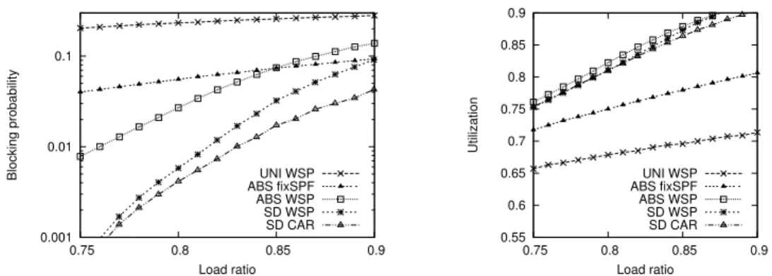
5.2 Wavelength Operating Modes . . . 84
5.3 Simulation Results . . . 86
5.4 Conclusion . . . 88
CHAPTER 6 DIMENSIONING DYNAMIC OPAQUE NETWORKS FOR LINK FAILURE RESTORATION . . . 89
6.1 The Cost of Protection . . . 90
6.2 Impact of Link Failures on Restoration . . . 91
6.3 Redimensioning and Discussion . . . 93
6.4 Conclusion . . . 94
CHAPTER 7 DIMENSIONING MULTIPLE DYNAMIC OPAQUE NETWORK DOMAINS . . . 95
7.1 Problem Description . . . 96
7.2 Multi-Domain Network Dimensioning . . . 98
7.3 Several Routing and Dimensioning Techniques . . . 100
7.4 Fairness Measurement . . . 102
7.5 Simulation Results and Discussion . . . 104
7.6 Conclusion . . . 108
CHAPTER 8 DIMENSIONING AND ROUTING FOR DYNAMIC WAVELENGTH SERVICES ON TRANSLUCENT NETWORKS . 111 8.1 Problem Description . . . 112
8.2 Differentiation to the Hose Model for VPN Traffic . . . 115
8.3 Optimization Techniques . . . 116
8.4 Lower Bound Computation and Heuristic Optimization . . . . 128
8.5 Volatility Analysis . . . 140
8.6 Sufficient Nonvolatile Conditions . . . 144
8.7 Numerical Results . . . 146
8.8 Conclusion . . . 152
CHAPTER 9 RELATED WORK . . . 154
9.1 Network Dimensioning . . . 154
9.2 Online Routing . . . 156
9.3 Multiple Network Domains . . . 159
9.4 Heuristic Optimization . . . 160
CHAPTER 10 CONCLUSION . . . 161
REFERENCES . . . 165
LIST OF ABBREVIATIONS
ASPF Adaptive Shortest Path First Routing ATM Asynchronous Transfer Mode
BAL Balanced basic dimensioning algorithm B&R Bridge and Roll
CAR Congestion Aware Routing COL Competitive Online Routing
CSR Concatenated Shortest path Routing D/MUX De/Multiplexing
DBR Design Based Routing DPP Dedicate Path Protection
DWDM Dense Wavelength Division Multiplexing E-NNI External Network-Network Interface E2E End-to-End global SPF
ER Edge Routers
FPLC Fixed-Paths Least-Congestion
GMPLS Generalized Multi-protocol Label Switching
GA Genetic Algorithm
GAF Genetic Algorithm with Fixed routes GS Global Shortest path dimensioning
ILP Integer Linear Programming
IS Independent Shortest path dimensioning
LC Liquid Crystal
LER Label Edge Router LLD Least Loaded Routing
LWR Least Resistant Weighted Routing LSP Label Switched Paths
LSR Label Switched Router
MEAN Incremental dimensioning algorithm using Mean scaling MEM Micro-Electronic-Mechanical
MIR Minimal Interference Routing MPLS Multi-protocol Label Switching NP Non-deterministic Polynomial-time NS Normalized Shortest path dimensioning nE2E Normalized End-to-End global SPF OOO Optical-Optical-Optical
OEO Optical-Electronic-Optical
OPT Optimization
OT Optical Transponder OXC Optical Cross-Connect PBR Profile-Based Routing PCE Path Computation Element QoS Quality of Service
RA Single Routing Area REGEN Regenerator
RFR Reduced Flow Routing
RWA Route and Wavelength Assignment
RSVP-TE Resource Reservation Protocol - Traffic Engineering SA Simulated Annealing algorithm
SAF Simulated Annealing algorithm with Fixed routes SDH Synchronous Digital Hierarchy
SDR State Dependent Routing
SD Incremental dimensioning algorithm using Standard Deviation scaling
SLA Service Level Agreement
SONET Synchronous Optical Networking SPF Shortest Path Routing
SPG Shortest Path Graph SPP Shared Path Protection
SWP Shortest Widest Path Routing TSL Topological Shortest path Length TSP Topological Shortest Path
VPN Virtual Private Network
WDM Wavelength Division Multiplexing WSP Widest Shortest Path Routing WSS Wavelength Selective Switching
LIST OF SYMBOLS
N Set of nodes.
E Set of links.
Ce Current residual capacity of link e ∈ E. C is the set of all links’ capacities.
Ve Current available capacity of link e∈E.
Ue Current used capacity of link e∈E. Ue =Ce−Ve.
Be Basic dimensioning capacity for each link. B is the set of all links’ capacities.
Xe Incremental dimensioning capacity for each link. Xis the set of all links’ capacities.
σe Statistic standard deviation of link capacity Be. σ is the set of all links’ standard deviations.
R Set of all end-to-end request pairs. R ⊆N ×N.
λ Mean arrival rate per pair. λi is a random arrival rate for a pair.
µ Mean departure rate per pair. The average holding time, 1/µ. µi is a random departure rate for a pair.
T Traffic matrix.
T SLr Topological shortest path length for a pairr.
T SPr Topological shortest paths set for pairr.
SP Gr Topological shortest path graph for pair r. SP Gr =∪p∈T SPrp.
fr(C) Maximum flow on SP Gr with link residual capacity C.
MCr(C) Set of links forming the minimum cut of a pairr with link residual capacity C.
u Projected traffic load ratio. u∈(0,1].
l Offered traffic load ratio. l > 0.
ǫ Traffic evolution factorǫ∈[0,1].
α Network misdimensioning factorα ∈[0,1].
ξ Incremental dimensioning scheme in{MEAN, SD}.
β Routing scheme in {SP F, W SP, LRW, CAR}.
SP Fr(C) Set of all shortest available paths of a pair r based on current residual capacity C.
Pi(C) Set of all available paths of a pair r based on current residual capacity C.
γp Path congestion cost.
η Congestion threshold.
dc,li Opportunity cost for a link with loadl, total capacityc, and current capacity i.
N′ Set of border nodes in the local network. N′ ⊂N.
S′ Set of foreign border nodes. S′ ⊂S,|S′|=|N′|.
C′
e Total capacity of link e∈E provisioned for the external traffic.
CI
b Total capacity of inter-domain link connecting border nodes b ∈
N′, b′ ∈S′ provisioned for the external traffic.
T′
L Equivalent external traffic matrix on the local network.
pn,s,b The probability that borderbis used to connect a local noden∈N to a foreign node s∈S. Pb∈N′pn,s,b = 1.
p Route. p={Vp, Np}, where Vp is the set of virtual links, andNp is the set of regen nodes.
l Link (or virtual link) distance.
W Ordered wavelength set (1 to|W|) in a DWDM fiber.
We,w Binary ILP variable. We,w = 1 if wavelength w ∈ W is allocated on link e∈ E; We,w = 0, otherwise.
Rn Nonnegative integer ILP variable for the number of REGENs at noden ∈ N.
CC Common cost per wavelength per mile. RC Regenerator cost per device.
C() Cost computation function. D Set of demand matrices.
M Set of maximal demand matrices. M ⊆ D. S Set of reduced demand matrices. S ⊆ M.
Ds The sth demand matrix. Ds ∈ D.
ds,t The tth demand of the sth demand matrix. ds,t ∈Ds.
N(d) The node pair (i, j) for demandd. In a context without confusion,
N(d) can represent a unique demandd. P(i,j) Set of routes for the node pair (i, j).
Xp,d Binary ILP variable. Xp,d = 1 if route p ∈ PN(d) is selected for demand d; Xp,d= 0, otherwise.
A Route allocation for all demands (in demand-route tuples) without wavelength assignment. |A| is the number of all demands. A[x:y] represents the list of xth to yth demand-route tuples.
A(d) Route allocation for demandd in allocation A.
A Set of all possible route allocations without wavelength assignment.
Aw Wavelength assignment for route allocationA ∈ A. A set of solved
CHAPTER 1
INTRODUCTION
In recent years, optical networks have evolved toward higher bandwidth, integrated routing planes, and flexible reconfiguration. At the same time, the request for on-demand and high-bandwidth connection services emerged from multiple application domains, such as cloud computing, video content hosting, and enterprise private networks. These applications drive the need for efficient management techniques for dynamic wavelength routed optical networks.
This chapter provides background on the technological advances, a sum-mary of new challenges, and the contributions of this thesis.
1.1
Background
Optical networks have evolved over the years to provide higher data-rate services in a cost-effective manner [1, 2]. Dense Wavelength Division Multi-plexing (DWDM), the major technology behind today’s backbone networks, has improved over the years to support higher data transmission rates per wavelength, larger numbers of wavelength channels multiplexed on a single fiber, and longer photonic signal transmission distances. These efforts greatly reduced the unit bandwidth cost and made high-bandwidth connections more affordable to a large number of customers.
Higher layer protocols, especially the IP layer, have become more closely integrated with the photonic layer. Traditionally, there were multiple digital layers in between for routing and grooming IP traffic on the optical trans-port. Synchronous Optical Networking (SONET) and Synchronous Digi-tal Hierarchy (SDH) are typical electronics-optical networks that transport Asynchronous Transfer Mode (ATM) traffic on optical networks. For a long time, ATM networks were the primary method of carrying voice data and
IP traffic. Today, however, the volume of IP traffic has outgrown that of other traffic by several orders of magnitude due to the growing popularity of Internet applications. IP is now the primary technology to support with the photonic layer.
Simplifying network protocol stacks for supporting IP traffic cheaply has become the technology priority for many network providers. Generalized Multi-protocol Label Switching (GMPLS) [3] was developed to provide sig-naling capability to directly reserve wavelength paths on WDM networks or SONET-like networks. Border Gateway Protocol (BGP) can be built upon GMPLS-over-WDM to carry regional Internet traffic. Further, a carrier-grade Ethernet standard is under development so that WDM networks, to-gether with other transport technologies, can directly transport Ethernet frames. With integrated control planes, the photonic layer can be more seamlessly connected to the user layer, and traffic at higher layers can have a more direct influence on the photonic layer.
Route configuration on photonic networks has become more flexible. In the past, route provisioning at the optical layer required intensive manual work; therefore, backbone networks were managed statically and did not allow frequent connection changes. Today, reconfigurable photonic devices— such as Reconfigurable Optical Add-Drop Multiplexers (ROADM), Micro-ElectroMechanical (MEM) photonic cross-connects, and tunable lasers—are widely used in core photonic networks [4, 5], greatly increasing the dynamic capability and transparency of the optical network. The GRIPhoN research testbed being developed at AT&T Labs can configure an optical route auto-matically in a few minutes and reroute a photonic path using a bridge-and-roll technique [6].
Recently, practical interest in providing on-demand wavelength connection services for future IP customers has grown [7, 8]. The emergence of relatively short-duration applications that require high data rates for video delivery, health care applications, etc. [9], has increased the dynamic variability of traffic. However, building and upgrading optical networks in response to frequent short-term traffic changes (i.e., hours and minutes) is expensive and impractical. For long-haul optical networks, expensive construction is needed to lay new fibers. Adding more active wavelength channels includes
even months, which makes it difficult to change as frequently as traffic varies. Therefore, the network provider must have sufficient equipment on hand to route dynamic traffic.
Although the majority of current long-haul optical networks remain stati-cally provisioned, general discussions of dynamic WDM channel provisioning dates back ten years [10]. The study in [11] showed that a dynamic network (called Intelligent Optical Network (ION) by the authors) could potentially save up to 80% capacity relative to the current static optical network (re-ferred to as Optical Transport Network (OTN)) for dynamic demands. The practical interests of providing on-demand wavelength connection services for future IP customers have revived research into online, link-state-based routing and load balancing on optical networks to supplement statically op-timized paths. Correspondingly, the underlying physical networks should be provisioned in response to the current and expected growth of dynamic traf-fic demands while simultaneously allowing robust adaptation to load changes and different network topologies.
1.2
Network Resource Management
Resource management for dynamic systems addresses three issues: traffic load characterization, network dimensioning, and online routing. Traffic load characterization involves finding a model to describe the amount of traffic in relation to network resources. Network resource dimensioning involves the distribution of equipment at initial setup or the upgrading of hardware on rare occasions. Online routingselects and allocates a route when a connection request arrives. As the frequency of demand variations (which change on an hourly or minute-based timescale) outpace the hardware upgrade speeds (which change on a days or weeks timescale) for new installations, it becomes less likely that a system can stay at the optimal point between equipment upgrades. Therefore, both the management of long-term load projection using resource dimensioning and short-term load fluctuation using online routing must occur. The goal is to improve performance and robustness of networks under load variations to reduce the need for resource reallocation and rebalancing.
Dimensioning for online, state-based routing schemes is challenging. Pre-vious studies on traditional circuit-switching networks tried to solve routing and dimensioning problems together by planning an optimal path (or a few alternative paths) for each demand. Many models were proposed to approx-imate the steady state blocking probability in such networks [12, 13, 14, 15]. Analytical approaches for fixed-path routing [16] can be useful for traditional telephony networks where traffic has a strong correlation to geographic fac-tors; however, these are not appropriate for data networks [17]. New fixed-point approximation techniques for routing online traffic on optical networks is difficult to scale to large mesh networks. To reduce the network state, a preselected path set is still used to approximate state-based online routing, and some routing preferences are ignored [18, 19, 20]. In fact, these approx-imations do not sufficiently capture the path selection preferences of online routing algorithms, which can make a substantial difference in performance results [20, 21, 22].
1.3
Thesis Contributions
This dissertation develops efficient network resource provisioning solutions (including resource dimensioning and online routing algorithms) through a combination of analysis and simulation. I built event-driven network simula-tors to study the quantitative relationship between network resource dimen-sioning and online routing. Traffic load characterization, dimendimen-sioning, and routing were considered jointly in order to achieve an optimal solution.
The thesis first presents efficient resource dimensioning algorithms on op-tically opaque networks for stochastic dynamic traffic. I then propose an analytical model of the opportunity cost for accepting a connection with a dynamic routing algorithm. Based on the model, I develop novel rout-ing algorithms with efficient implementation, and the algorithms are robust to network variables, such as topology and capacity. The resource dimen-sioning technique can be applied to translucent networks, restorable opaque networks, and multiple opaque network domains.
an optimal network resource provisioning. On problems of current practical interest, my methods achieve an average of 8% overhead above lower bounds of optimal values. I also introduce theoretical analysis of the traffic model and leverage properties that can significantly reduce optimization time. This work is the first to evaluate the benefit of using an optical bridge-and-roll technique (a route changing technique for minimizing signal loss that sets up the new route before removing the old route) for dynamic wavelength services. Despite the benefits, the bridge-and-roll operation requires that the resources for the new route must be available before the old route is torn down. The analysis shows that optimal provisioning cannot always satisfy the bridge-and-roll condition with optimized resources. I derive provable bridge-and-roll safe provisioning technique and measure negligible overhead for ensuring bridge-and-roll rerouting on real-scale network simulations.
The remaining chapters are organized as follows. Chapter 2 provides back-ground information on dynamically routed optical opaque and translucent networks, cost models, Poisson traffic models, dynamic wavelength services models, typical routing algorithms, network topologies, assumptions, and simulation methodologies. Chapter 3 introduces load metrics and dimen-sioning algorithms for Poisson-loaded opaque networks. In Chapter 4, I pro-pose a novel flow-based online routing algorithm, an opportunity cost model for optimizing threshold-based congestion control routings, and an oracular optimal routing. Chapter 5 describes the performance of the dimensioning algorithms presented in Chapter 3 on translucent networks and evaluates the resource distribution for four different wavelength operating modes. Chap-ter 6 presents a redimensioning technique for a single-link failure restorable network, and Chapter 7 develops dimensioning algorithms for two separately managed optical networks and discusses fairness issues. I suggest efficient techniques to tackle a challenging resource optimization problem for dy-namic wavelength services and analyze the applicability of optical rerouting techniques Chapter 8. Chapter 9 explores related work, while Chapter 10 concludes the thesis.
CHAPTER 2
OPTICAL NETWORK MODELS AND
MANAGEMENT
This chapter discusses foundational concepts, including network models, cost models, traffic models, and route management technologies.
2.1
Translucent Networks
In optical network systems, the term “transparent” refers to photonic cir-cuit switching without per-packet electronic processing; all optical switch-ing is also called optical-optical-optical (OOO). The term “opaque” refers to switching that involves optical electronic conversion and regeneration in which optical signals are converted, corrected, and retransmitted. Opaque switching, also called optical-electronic-optical (OEO) switching, was used at all nodes in early optical networks when all-optical switching devices were too expensive and the insertion loss was too high, making long photonic transmission without electronic regeneration impossible. With substantial improvements in photonic devices, today’s transmission systems extend the distance and switching hops between a pair of optical transmitters and re-ceivers.
Given these changes, an emerging model of “translucent” networks has become popular. In this model, optical signals are circuit-switched photon-ically at some nodes and electronphoton-ically regenerated at other nodes, as nec-essary. Reconfigurable Optical Add-Drop Multiplexer (ROADM) networks are a type of translucent network widely used in practice. Dense Wave-length Division Multiplexing (DWDM) technology, harnessing the reconfig-urable power of tunable lasers and photonic cross-connects, has emerged as a key component in future dynamic ROADM infrastructures. This section
work architecture. A detailed description of the physical characteristics of the transmission system can be found in [5, 23, 24, 25, 4].
2.1.1 Reconfigurable Optical Add-Drop Multiplexer Networks
In a wavelength division multiplexing system, data packets are modulated into analog optical signals and multiplexed onto a specific wavelength fre-quency of a DWDM signal. The signal is transmitted through a long-reach fiber system that connects remote switching nodes. DWDM technology re-markably improves the efficiency of optical systems by enabling a fiber link to carry 40 to 80 different wavelength channels at the same time. An optically reconfigurable network consists of ROADM as nodes and DWDM fibers as links. A typical backbone ROADM network is a mesh topology that inter-connects nodes at city’s level. Each city may have one (or more, depending on the city population) switching node at the carrier’s central office. Each fiber link transmits high-power optical signals for hundreds of miles without electronic signal regeneration.
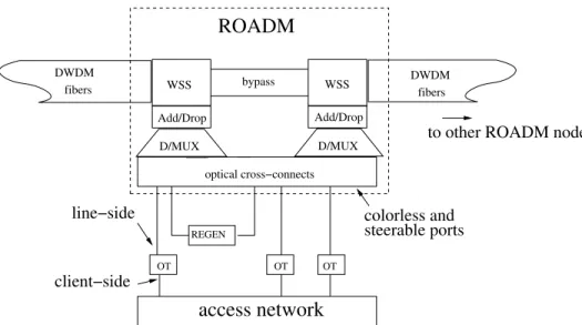
Figure 2.1 shows the architecture of a ROADM node on the GRIPhoN testbed that is being developed at the AT&T Labs Research. All optical links are bidirectional such that each port of the shown devices connects to a pair of fibers, one for each direction. The ROADM node is fully reconfigurable: any wavelength from one DWDM input can be switched to other available DWDM ports or add/drop ports. The ROADM has colorless and steerable add/drop ports, enabling OTs and REGENs to connect to any available add/drop ROADM port and any available wavelength color.
GRIPhoN ROADM nodes achieve reconfigurability using Wavelength Se-lective Switches (WSS). A WSS can deflect a wavelength channel from one port to the other. Some devices use an array of electronically configurable MicroElectroMechanical (MEM) mirrors as switching components. Newer devices use Liquid Crystal (LC)-based channel blockers that can be con-trolled to select pass-through wavelength channels. The wavelength channels that need to drop locally are demultiplexed into individual wavelength sig-nals that are carried by one fiber per wavelength channel. Typically, these are low-power optical connections that transmit short-reach signals within tens of meters.
D/MUX REGEN OT OT OT DWDM fibers DWDM fibers steerable ports colorless and
to other ROADM node ROADM line−side client−side bypass Add/Drop Add/Drop WSS optical cross−connects WSS access network D/MUX
Figure 2.1: A ROADM node architecture.
An optical transponder (OT) has a local interface that connects to the optical ports of access routers and a line-side interface (high-power laser port) that connects the ROADM network. A local signal is electronically transcoded at an OT and sent through its laser for long distance transmis-sion. Today’s OTs are wavelength tunable, i.e., an OT can receive from any wavelength channel of the demultiplexed DWDM signal and send to another wavelength channel. A 3R regenerator (REGEN) receives the data from a wavelength channel and resends the same data to another wavelength. Physi-cally, a 3R REGEN is equivalent to a pair of optical OTs whose customer-side ports are short-connected. However, a REGEN lacks customer-side ports, so it cannot be used as an OT.
Traditionally, ROADM nodes are non-steerable or partially steerable be-cause OT/REGENs can connect to only one wavelength channel of one add/drop ports. GRIPhoN ROADM nodes achieve full steerability by us-ing an optical cross-connect. Therefore, the OTs and REGENs can con-nect to any of the wavelength channels of the D/MUX add/drop ports of any direction. This design provides the opportunity to share OT/REGENs throughout the entire node.
The access network interfaces the ROADM network to high layer protocols, such as SONET/SDH, ATM, IP or carrier-grade Ethernet. In practice, the
per fiber for tens of meters. The access network provides an electronic layer built on top of the photonic layer.
2.1.2 Route Provisioning
A wavelength connection is set up between a pair of OTs installed at source and destination ROADM nodes. The route must be a simple path; no node is visited twice. Figure 2.2 shows an example route. Intermediate ROADM nodes, which route the connection through optical bypass cross-connects, are called “bypass” nodes. If the connection distance exceeds the maximal optical reachability for the network system, some intermediate nodes serve as “regen” nodes and cross-connect the connection through a 3R REGEN. In order to regenerate a signal, the connection is received by a REGEN through a drop port and resent by the same REGEN through an add port. The route segment between a pair of OTs or REGENs is called an “optically transparent segment.” Except for the end nodes, all intermediate nodes in an optically transparent segment are bypass nodes. Therefore, wavelength continuity is enforced within a segment. The wavelength can change from segment to segment using the REGEN.
ROADM networks are managed centrally and completely circuit switched. ROADMs, optical cross-connects, OTs (both line-side and customer-side), and REGENs are all remotely configurable. On the GRIPhoN testbed, wave-length connections can be set up and torn down in a few minutes, which makes it possible to provide a dynamic wavelength service. If a customer owns a few OTs at different ROADM nodes, the network allows the cus-tomer to reconfigure the optical network topology freely by creating and removing connections on the reconfigurable ROADM network.
2.1.3 Reachability and Virtual Link Graph
Optical reachability is the maximum distance of an optically transparent segment allowed for a system. For 10Gbps or 40Gbps systems, reachability is typically 1500 km (932 mi). A virtual-link graph simplifies the routing of optically transparent segments with reachability constraints. The original virtual-link idea was explained as express links in [26]. To create a virtual
OT OT
ROADM ROADM ROADM ROADM
REGEN optical transparent
segment
bypass node regen node
add/drop node add/drop node
fiber fiber fiber
customer customer
Figure 2.2: Bidirectional wavelength connection. The connection includes two optically transparent segments. The first segment routes on a red wavelength. The second segment routes on a blue wavelength.
200mi 600mi 300mi
(a)
(b)
(c)
200mi 600mi 300mi
900mi 800mi
Figure 2.3: (a) Physical graph with link marked with fiber distance (in miles). (b) The corresponding virtual-link graph for a 40Gbps system (reachability of 932 mi). Virtual links are also marked with fiber distance. (c) Example customer route on the virtual-link graph. The route passes two transparent segments. The dashed wavelength is marked for use by all links in the graph. A REGEN at the solid node connects two segments. The cost of the path is 150 + 1100100070 = 227.
link graph, a virtual link is created for every reachable optical transparent segment (including each individual physical link). All virtual links that pass the same physical link share the wavelength resources of the physical link. A route can be created on the virtual-link graph. The physical route that maps to the virtual-link route must be a simple path. A REGEN must be used at each node that connects two virtual links. Figure 2.3 shows an example.
2.1.4 Photonic Bridge-and-Roll Rerouting
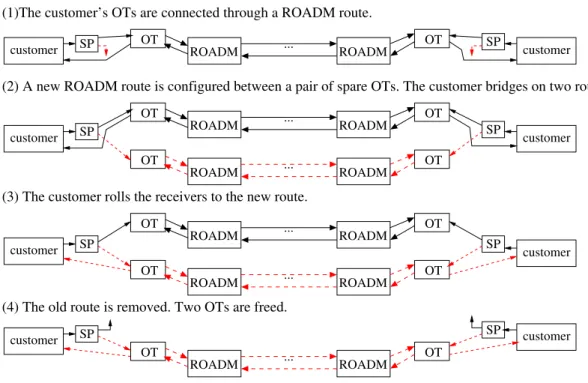
Optical bridge-and-roll (B&R) rerouting is supported by the GRIPhoN testbed. Figure 2.4 illustrates the B&R process. A new route is set up between two
OT ROADM ROADM OT OT ROADM ROADM OT OT ROADM ROADM OT OT ROADM ROADM OT OT ROADM ROADM OT customer SP customer SP customer SP customer customer customer SP SP SP OT ROADM ROADM OT customer SP SP customer ... ... ... ... ... ... (3) The customer rolls the receivers to the new route.
(4) The old route is removed. Two OTs are freed.
(2) A new ROADM route is configured between a pair of spare OTs. The customer bridges on two routes. (1)The customer’s OTs are connected through a ROADM route.
Figure 2.4: Illustration of optical B&R operation steps. A 50/50 optical passive splitter (SP) is preinstalled at the customer’s transmission side. tical passive splitter is preinstalled at the customer’s transmission port. The customer then has the opportunity to “bridge” two OT routes at any time without interrupting the transmission. Once the customer bridges the old and new routes, the receivers are quickly “rolled” to the OTs of the new route. Finally, the old route is taken down. In order for B&R to work, there must be one spare OT available at each node, and the new route must be resource disjoint from the old route. The GRIPhoN testbed demonstrated that the Ethernet packet loss period is about 8 milliseconds in a photonic layer B&R experiment [6].
2.1.5 Cost Model
The capital expense of a ROADM network consists of the cost of OTs, REGENs, ROADM ports, and DWDM fibers. Since the cost of tunable OTs/REGENs is relatively high and increases linearly with the load of net-work connections, they are counted as a per-equipment cost. The rest of the equipment, shared by all wavelengths, has to be preinstalled. Therefore, it is modeled as a common cost and prorated in wavelength-miles. The current
normalized cost (based on vendor’s price) for 40Gbps systems is 100 for an OT, 150 for a REGEN, and 0.07 per wavelength per mile. The cost of the sample route in Figure 2.3(c) is 227. The REGEN cost is nearly double the common cost for this route.
2.2
Opaque Networks
Typically, IP networks can be built directly upon WDM networks. Any link between two IP routers is, in fact, one or more wavelength routes that may have multiple OOO or OEO hops, where no electronic processing occur at the IP layer. IP-WDM network architectures have become increasingly popular as IP traffic (VPN channels) has dominated the usage of backbone networks. The traditional opaque network model can apply to these VPN networks, as optical signals in fact are electronically processed and circuit switched at every VPN node. Wavelength continuity does not impose on the network as a routing constraint.
2.2.1 Generalized Multi-Protocol Label Switching (GMPLS)
A GMPLS network [3] is an opaque network. GMPLS builds an electronic network interface on the lower optical network of the IP layer. Each link on the GMPLS network is an optical lightpath that consists of one or more hops. Its control platform extends traditional MPLS [27] to support rout-ing through various physical infrastructures, includrout-ing synchronous optical networks (SONET/SDH) and photonic networks (DWDM), aiming at in-tegrating multiple network carriers into a single control structure. As an extension of MPLS, GMPLS also provides signaling for explicit routing for connectionoriented optical networks. The resource reservation protocol -traffic engineering (RSVP-TE) [28] protocol provides resource reservation or non-reservation routing through label switched routers (LSRs), including establishing label switched paths (LSPs), preemption, and loop detection functions. According to [7], GMPLS networks employ dynamic routing and signaling mechanisms so that LSPs can be established and terminated on
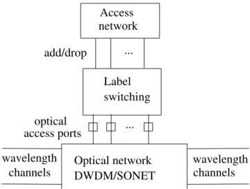
channels Optical network DWDM/SONET Label switching Access network add/drop access ports optical ... ... wavelength channels wavelength
Figure 2.5: A label switching node structure.
Figures 2.5 depicts the node architecture of a GMPLS network. The label switching router (LSR) has optical-electronic interfaces to the underlying op-tical networks, such as DWDM or SONET. Local access (often implemented as a label edge router (LER)) is an interface to an IP network. LER generates end-to-end routing requests, and LSR forwards traffic. Practically, LER and LSR together can be conceptualized as an electronic switch that integrates multiple network layers and provides routing functionality at the IP layer. However, in some networks, some nodes have either LER or LSR. The nodes without an LER do not generate new traffic. Currently, the industry is also developing standards for carrier-grade Ethernet that allow the optical layer to carry native Ethernet frames. For a GMPLS on a ROADM design, the label switching module accesses the ROADM network through OTs. The label switch processes at the packet level and forwards packets according to the labels. This thesis considers only the type of networks that switch at the data rate of one wavelength channel. It does not discuss electronic traffic grooming or sub-wavelength routing.
2.2.2 Cost Model
This thesis uses a per-wavelength cost model for opaque networks. One unit cost is assigned to each wavelength channel provisioned between any pair of nodes. For wavelength routing, the cost of a route simply counts the number of hops. Such simplification is reasonable because the per-wavelength
pho-tonic equipment comprises the majority of the network cost. The percentage continues to grow as the data rate increases. A projection of the capital expense of future 40 Gbps network systems showed that 91% of the cost is at the terminal devices (switching ports, routers, transponders, regenerator cards) [24]. Amongst terminal devices, electronic routing/grooming takes 40%. If we subtract the electronic part, OT and REGEN constitute 83% of the photonic cost.
2.2.3 Online Routing Algorithms
The dynamic routing problem has been extensively studied for circuit-switched ATM networks. Dynamic routing in a mesh network involves selecting an available path on the arrival of an end-to-end connection request, based on the current network capacity. A connection request is initiated by a source-destination node pair. Without loss of generality, we consider only bidirec-tional connections. For abbreviation, “node pair” or “request pair” refers to a pair of nodes that initiates a connection request.
Adaptive shortest path first (ASPF) routing is a simple solution that se-lects an available path with the fewest hops. The connection request is dropped if no SPF paths can be found. Many other heuristic solutions have been proposed to improve connection acceptance rates using an estimate of the traffic load. This section introduces a few such online routing algorithms (Algorithm 2.1).
Some algorithms select routes exclusively from the available shortest paths on the residual graph. Widest shortest path first (WSP) routing picks the path of the largest residual capacity at the bottleneck link. The WSP+1, a one-hop relaxed WSP variant, chooses the widest path among all paths within shortest hops plus one. Further ties are broken arbitrarily since the choice would have little impact on the capacity distribution of future residual networks.
Some algorithms select routes from available paths of any length. The SWP algorithm chooses the shortest hop path from all paths with the widest residual bottleneck capacity. Least resistant weighted (LRW) routing [29] chooses the minimum cost path as defined by the sum of the ratios of
to-Algorithm 2.1: Routing algorithms
1 beginWSP
2 foreachp∈SP Fs,d(C)do 3 γp←mine∈pCe;
4 Pick the widestpath←arg maxpγp; 5 beginSWP
6 foreachp∈Ps,d(C)do 7 γp←mine∈pCe;
8 Widest path setQ∪arg maxpγp; 9 Pick the shortestpath←arg minp∈Q|p|; 10 beginLRW 11 foreachp∈Ps,d(C)do 12 γp←P e∈p (Be+Xe) Ce ;
13 path←arg minpγp; 14 beginMIR
15 foreach r∈R do
16 Compute min-cut link set M Cr(C); 17 foreachp∈Ps,d(C)do 18 γp←P e∈p P r6=(s,d):e∈M Cr(C) λ µ;
19 path←arg minpγp; 20 beginSDR 21 foreachp∈Ps,d(C)do 22 γp←P e∈p ErB(Ce,le) ErB(Ue,le); 23 q←arg minpγp; 24 if γq > ηthen
25 Reject the connection;
26 else
27 Accept the connection on routeq; 28 beginCOL 29 foreachp∈Ps,d(C)do 30 γp←P e∈pυ −CeVe; 31 q←arg minpγp; 32 if γq > ηthen
33 Reject the connection;
34 else
(MIR) [30] uses the flow of information to compute network weights for rout-ing. The computation of complete MIR routes is NP-hard. Therefore, an online version of MIR was proposed to approximate the optimal solution while reducing computation complexity. MIR first computes the min-cut link set for the flows of all other node pairs excluding the current one. Then, MIR computes the link cost by summing the min-cuts that involve this link of all other pairs. The link cost is further weighted by the predetermined “importance” of a pair. I use the expected Poisson load for the parameter. Finally, MIR chooses the path with the minimum total weight. The compu-tational time for each request is three orders of magnitude higher than for non-flow-based algorithms.
There are also threshold-based routing algorithms. State-dependent rout-ing (SDR) [31] attempted to compute the best route usrout-ing a Markov decision process. As the model quickly becomes intractable, a link cost model is proposed to approximate the analytical solution. The cost of each link is computed by ErB(Ce,le)
ErB(Ue,le), where ErB(Ce, le) is the Erlang-B blocking formula,
and le is the link load estimation. Link load is estimated using a SDRAdapt algorithm [32]. Basically, SDRAdapt periodically measures residual capacity on each link and updates estimated link load in a sliding window fashion. SDRAdapt requires the selection of two parameters: a scan interval δ and a sample number ∆; the authors picked δ = 0.5 and ∆ = 30. However, the result is sensitive to these parameters, and better results were obtained using δ = 0.05 and ∆ = 50 (Chapter 4). The difference is due to the lack of normalization of timescales between papers.
Gawlick et al. [33] proposed a throughput-competitive online routing and admission control algorithm (COL). The original version of the algorithm re-quired knowledge of the actual holding time of each connection. The authors therefore proposed a practical version in which each link cost is computed by υ−CeVe. However, the determination of υ is nontrivial, and the result is
sensitive to υ [32]. The authors did not provide any effective way to choose
2.3
Typical Network Topologies
As carrier-grade networks often contain proprietary information and are kept away from public access, this thesis uses open topologies (mostly from re-search projects) that provide characteristics similar to practical backbone networks. Figure 2.6 shows the backbone topologies for simulating the per-formance of optical opaque network models. NJ LATA provides a good case study for performance evaluation on small networks. The other networks all serve regional telecommunication needs. COST 239 interconnects major cities in Europe. NSFNET was built to connect academic supercomputing centers across the U.S for research purposes.
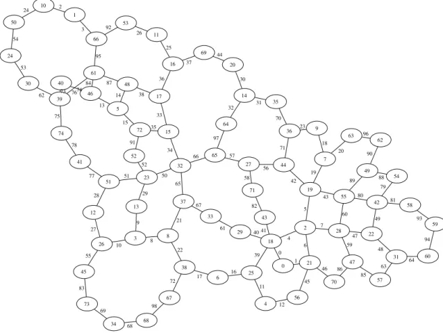
Figures 2.8 and 2.7 show the topology of U.S. CORONET, chosen as the backbone topology for simulating translucent networks. CORONET was created by a Telcordia-AT&T team to mimic a typical large international core network [34]. We use the U.S. contiguous part of CORONET, which consists of 75 nodes and 99 links. Table 2.1 shows the mapping of CORONET nodes to U.S. cities. This thesis targets a 40Gbps ROADM system that has the maximal optical reach of 932 miles. I proportionally scaled down the link distance by 75% of the original CORONET to fit the single hop reach of today’s 40Gbps system. Table 2.2 lists the new link distances in miles that are used in this thesis.
2.4
Traffic Models
2.4.1 Poisson Traffic
This thesis uses the Poisson model to generate connection request arrivals, but my algorithms do not depend upon this choice. Rather, the Poisson model is chosen because the burstiness of traffic on backbone networks is usu-ally suppressed by huge amounts of aggregation of higher layer services [35]. The real traffic distribution remains unknown as few practical dynamic op-tical backbones exist today, and traffic statistics from carriers are often pro-prietary information.
Unless otherwise specified, all node pairs in a network generate traffic arrivals. Each node pair initiates a connection arrival following a Poisson
1 2 3 8 9 10 6 5 0 4 7 1 2 6 9 18 3 15 16 14 19 13 20 7 4 12 8 21 5 17 22 10 11 0
(a) NJ LATA the New Jersey Local Access and Transport Area Network.
1 5 3 5 41 29 8 3 9 40 19 7 15 20 20 21 21 22 19 18 17 17 18 43 39 8 22 23 24 0 0 23 9 28 38 25 2 1 2 7 26 10 37 27 31 4 30 6 34 35 15 16 16 36 14 33 14 13 13 12 32 42 12 6 10 4 11
(b) NATIONAL the U.S. national network.
1 3 6 7 8 9 10 11 15 28 27 31 12 29 0 19 25 24 18 26 16 23 14 22 13 20 21 4 5 2 30 17 6 1 2 15 18 14 12 16 19 0 17 13 9 10 4 5 11 8 3 7
(c) ARPANET the Advanced Research Projects Agency Network. 3 0 9 12 13 14 17 1 35 36 15 11 34 16 2021 23 24 10 22 25 2 19 18 26 27 7 28 29 4 5 6 30 31 32 33 8 6 8 11 10 9 12 13 17 15 7 16 18 14 0 4 3 1 5 2
(d) COST 239 the Ultra-high Capacity Optical Transmission Network. 0 4 3 5 8 6 12 14 16 0 1 2 3 4 6 5 7 8 9 10 11 12 13 1 10 20 18 7 15 13 17 19 11 9 2
Figure 2.7: U.S. CORONET on the U.S. map. 0 18 0 21 1 25 39 29 40 43 41 56 45 70 46 1 10 2 66 3 50 24 2 4 6 19 5 28 7 44 42 55 43 60 47 59 3 8 8 13 9 26 10 38 22 37 21 23 29 45 55 4 11 12 5 46 13 48 14 72 15 61 84 87 6 16 17 67 72 7 19 9 18 63 20 36 23 71 11 16 25 53 26 17 36 69 37 92 12 27 51 28 51 32 50 52 52 14 20 30 35 31 64 32 44 70 65 97 15 35 33 34 38 65 66 33 61 71 82 22 47 31 48 42 49 57 63 60 64 80 54 79 58 81 91 24 54 30 53 39 62 73 83 27 56 57 58 86 85 67 40 73 74 74 75 34 68 68 69 98 76 95 41 77 78 59 93 49 89 88 62 90 96 94
Figure 2.8: U.S. CORONET. Optical translucent network topology with link and node numbers.
Table 2.1: U.S. CORONET node-to-city map.
# city # city # city
0 Abilene 25 Houston 50 Providence 1 Albany 26 Jacksonville 51 Raleigh 2 Albuquerque 27 Kansas City 52 Richmond 3 Atlanta 28 Las Vegas 53 Rochester 4 Austin 29 Little Rock 54 Sacramento 5 Baltimore 30 Long Island 55 Salt Lake City 6 Baton Rouge 31 Los Angeles 56 San Antonio 7 Billings 32 Louisville 57 San Diego 8 Birmingham 33 Memphis 58 San Francisco 9 Bismarck 34 Miami 59 San Jose 10 Boston 35 Milwaukee 60 Santa Barbara 11 Buffalo 36 Minneapolis 61 Scranton 12 Charleston 37 Nashville 62 Seattle 13 Charlotte 38 New Orleans 63 Spokane 14 Chicago 39 New York 64 Springfield 15 Cincinnati 40 Newark 65 St Louis 16 Cleveland 41 Norfolk 66 Syracuse 17 Columbus 42 Oakland 67 Tallahassee 18 Dallas 43 Oklahoma City 68 Tampa 19 Denver 44 Omaha 69 Toledo 20 Detroit 45 Orlando 70 Tucson 21 El Paso 46 Philadelphia 71 Tulsa 22 Fresno 47 Phoenix 72 Washington DC 23 Greensboro 48 Pittsburgh 73 West Palm Beach 24 Hartford 49 Portland 74 Wilmington
Table 2.2: U.S. CORONET link distance.
# mile # mile # mile # mile
0 252.7 25 252.3 50 517.8 75 153.1 1 570.9 26 95.0 51 98.3 76 102.1 2 207.8 27 284.5 52 238.4 77 224.0 3 175.7 28 322.6 53 139.7 78 287.8 4 850.1 29 119.9 54 94.2 79 99.5 5 485.8 30 344.4 55 184.9 80 851.8 6 327.7 31 124.0 56 235.5 81 19.3 7 707.7 32 268.2 57 353.2 82 145.0 8 199.7 33 144.9 58 313.8 83 206.8 9 329.4 34 133.1 59 371.9 84 145.1 10 415.6 35 582.8 60 525.0 85 431.0 11 211.5 36 179.2 61 196.0 86 166.8 12 107.7 37 143.4 62 22.0 87 355.2 13 134.4 38 221.0 63 167.9 88 703.3 14 288.6 39 324.6 64 113.0 89 915.9 15 50.4 40 415.5 65 221.3 90 209.3 16 375.1 41 275.2 66 355.3 91 142.6 17 110.5 42 690.3 67 283.4 92 109.0 18 546.8 43 548.5 68 297.8 93 57.9 19 660.0 44 80.4 69 97.4 94 335.2 20 636.6 45 723.3 70 426.3 95 167.8 21 264.3 46 379.3 71 421.0 96 333.2 22 436.9 47 372.2 72 490.0 97 108.0 23 554.2 48 290.0 73 18.2 98 295.6 24 59.9 49 217.5 74 149.7
distribution. The thesis does not differentiate connection requests of opposite directions. One arrival rate characterizes the load of each node pair. Existing connections depart in an exponential distribution.
2.4.2 Dynamic Wavelength Service
AT&T’s dynamic wavelength service model allows customers to create or remove a wavelength connection on-demand on a dynamic ROADM network. Customers own or lease a set of OT ports to access the network. They can choose to connect between their free OTs at different nodes in arbitrary ways. Every connection occupies one of the customer’s OTs at each end of the connection until the connection is released. The routes are preprovisioned at the design phase to guarantee 100% acceptance of valid connection requests. Network resources, such as REGENs and wavelengths, must be preinstalled so the customers can reconfigure their connections at any time and within a few minutes. A network can have many customers. But one customer is not allowed to connect to another customer’s OT ports. The demands of each customer are independent. No sharing of network resources between customers is considered.
2.5
Simulation Assumptions
This thesis assumes that the topology of the backbone network is given. In particular, we evaluate simulation results on a few existing backbone topolo-gies. Often, backbone networks are built along railways. The location of cities, costs of construction, and rights-of-way are all important factors in determining where to place fibers. The problem of network topology design is beyond the scope of this thesis.
The network is managed centrally. The route configuration time is shorter than the expected inter-arrival time. Each connection arrival/departure can be processed before the next arrival request. Bidirectional wavelength routes are automatically set up and taken down for each request. Each wavelength route occupies one wavelength channel on each link of both directions along the path until the connection terminates. Based on the routing policy and the current availability of wavelengths, the network either accepts or rejects
0 0.01 0.02 0.03 0.04 0.05 0.06 0.07 0.08 0 10000 20000 30000 40000 50000 Blocking probability
Number of arrival requests Sample average Warm-up period LRW SPF WSP RFR
Figure 2.9: Steady state performance on NJ LATA.
a connection request. No queuing/preemption/rerouting is assumed. We use the same route for connection requests from opposite directions. We assume that the traffic load changes slowly relative to connection arrivals and departures. Specifically, request arrival rates and hold times for connections allow sufficient time for signaling such that all new connections are routed based on up-to-date information about residual capacity for all links in the network. The dynamic network system can come sufficiently close to a steady state.
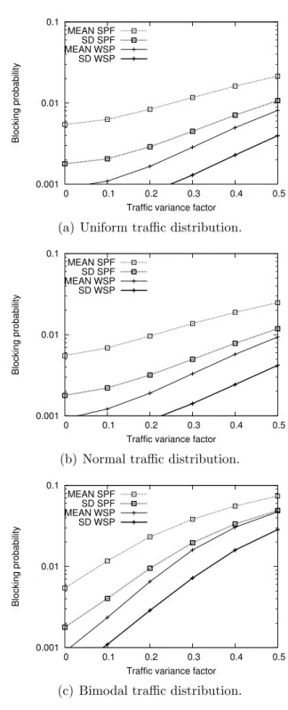
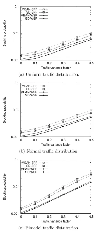
This thesis studies the performance of networks under traffic evolutions. To model various traffic demands, I introduce a traffic matrix space that includes all possible traffic matrices. The traffic matrix space is defined by an average arrival rate and a departure rate for each end-to-end pair. One traffic matrix in the space is generated by randomly selecting an arrival rate for each pair. The selection of an arrival rate follows uniform distribution, normal distribution, or bimodal distribution of the same mean and devia-tion. One departure rate is used for all connections. Connection arrivals and departures are modeled by Poisson processes. The arrival process follows the arrival rate of each pair from the traffic matrix. The departure process of any connection follows the departure rate. Each connection requests one wavelength capacity.
The blocking probability is sampled by averaging 5000 arrivals at steady state behavior. The simulation is repeatedly run until the 95% confidence interval is within ±5% of the value or the blocking probability is lower than
the test networks given our traffic load and all the algorithms considered, the system reaches a steady state after 20,000 requests.
CHAPTER 3
DIMENSIONING OPAQUE NETWORKS
FOR EVOLVING TRAFFIC
New Internet applications are increasingly generating high-bandwidth, short-lived demands. If network resources are available, establishing a lightpath on-demand takes only a few minutes on today’s reconfigurable optical networks. These demands thus create a more variable and unpredictable environment for long-term network planning. At the same time, upgrading backbone net-works is expensive and therefore occurs infrequently. Dimensioning network resources to sustain variable traffic demands for the long term requires fewer upgrades to achieve high performance but poses complex challenges.
Two kinds of dimensioning problems for optical opaque networks are pro-posed and studied in this chapter: (1) basic dimensioning, which allocates network resources for a newly built network; and (2) incremental dimension-ing, which allocates extra resources for future demand growth and variations. I propose new metrics to quantify the traffic load and the traffic pattern evo-lution for dynamically routed networks. I evaluate performance under load scaling, traffic evolution, and misdimensioning; a dimensioned network can sustain a much higher load while providing the same performance compared to misdimensioned ones. My approach is better adapted to traffic evolution than either a uniform allocation or the asymptotic optimization approach proposed earlier.
3.1
Load Definition
This section introduces network load metrics. Many previous studies still use the traditional Erlang unit to model traffic volume. An Erlang represents the use of a single voice channel; in practice, it has typically been measured by
However, on a dynamic mesh network, the number of calls does not clearly connect to network resources. We can linearly approximate the resources used per call using an average, but the scaling factor must be calculated for a specific topology and a specific traffic pattern on that topology. The Erlang definition is too simplistic to represent network loads adequately.
I propose a new load metric. I model the average network resources used by the expected traffic by the sum of Poisson load weighted by the topo-logical shortest path length for each request pair. Poisson dynamic traffic is assumed (see Section 2.4.1). LetN be the set of nodes andRbe the set of all end-to-end request node pairs. Each pair i∈R in the network is character-ized by the mean arrival rate λi, departure rate µi, and capacity demand 1. LetE be the set of links. Each linke ∈E is dimensioned with total capacity
Be +Xe, where Be is the capacity to support expected traffic, and Xe is the incremental capacity to support future traffic variations. The Xe portion can be deployed at a later time than the Be portion. Once both portions are installed, they are treated the same in the total volume Be+Xe. For a dimensioned network to support the expected traffic, the total basic capacity should equal the expected traffic volume, as shown in Equation (3.1).
X e∈E Be= X i∈R λi µi T SLi (3.1)
where T SLi is the topological shortest path length for request pair i ∈ R. The extra capacity, X = Pe∈EXe, is dimensioned for future traffic scal-ing and variations. Therefore, the projected traffic load ratio, u, is defined by Equation (3.2). u= P e∈EBe P e∈E(Be+Xe) (3.2) At routing time, the actual load ratio l can be greater or smaller than the projected load ratio.
3.2
Dimensioning Procedure
The dimensioning algorithm appears in Algorithm 3.1. Basic dimension-ing (Lines 1-12) computes basic capacity B, and incremental dimensioning (Lines 13-20) computes extra capacity X according to the type of
incremen-λ
Pattern change
λ1 λ2
Traffic matrix space
Normalized traffic matrix Load scaling
high load
low load
Figure 3.1: Traffic space and evolution model for two node pairs. The arrival rates are noted by λ1 and λ2.
tal dimensioning algorithm ξ ∈ {MEAN, SD} used. If the projected load ratio is u = 1, X = 0, no incremental dimensioning is needed. In general, the simulation-based basic dimensioning algorithm can handle any traffic distribution with a given mean for arrival rate, departure rate, and capac-ity demand. Algorithm 3.2 shows a simpler analytical version for Poisson traffic that can generate equivalent results. However, the simulation version can be easily extended to handle more complicated cases. For example, if a link/node is physically bounded by a maximum capacity, the routes can avoid these links when they are full.
In our model, the load characteristics of each request pair (λi, µi) are ran-domly drawn from a traffic space. The traffic space is characterized by an arrival rate, a departure rate, and a distribution that defines the probability of possible arrival rates. Let λ be the mean arrival rate and µ be the mean departure rate. Any traffic matrix is a point inside the whole space of all possible traffic matrices that can be generated from the distribution. Since the departure rates are assumed the same, the arrival rates are the varying values. Let T = {λi, µi}|R| denote a random projected traffic matrix that is drawn from the space. Figure 3.1 illustrates a traffic space model for two node pairs. Assume that the arrival rate follows a bounded uniform distri-bution of mean λ. The space is a square. Over time, the real traffic load can vary in both scale and pattern, which is characterized as traffic evolution in Section 3.3.
The average traffic load is defined in Equation 3.3 such that all arrival rates equal the mean arrival rate λ.
loadavg = λ µ X j∈R T SLj (3.3)
The load of a random traffic matrix can be either lower or higher than the average traffic load. In practice, estimation of projected traffic matrices is susceptible to measurement errors or obsolete data. In order for the dimen-sioning algorithm to be robust to traffic load changes, the arrival rates of a projected traffic matrix are adjusted proportionally so the new load equals the average load. Equation (3.4) shows the normalization. Given a traffic matrix, each arrival rate is scaled by a constant.
λni =λi loadavg P j∈R λj µjT SLj (3.4)
The goal of incremental dimensioning is to allocate extra capacity, perhaps at a later time, to adapt to traffic evolution. The method should increase capacity allocation without interfering with established connections (and re-sources).
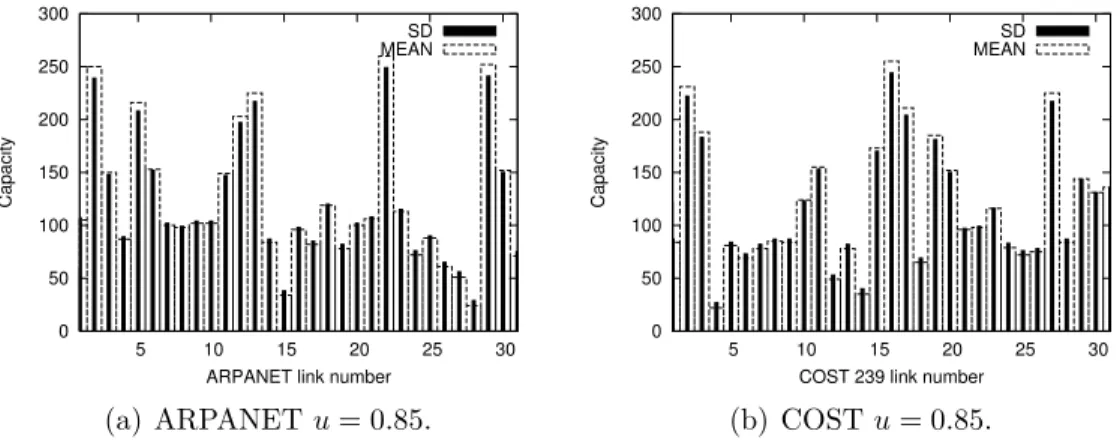
Two incremental dimensioning schemes (MEAN and SD) are proposed. The MEAN scheme increases each link’s capacity by an amount proportional to that capacity. MEAN over-dimensioning occursimplicitlywhen the offered traffic load ratio is smaller than the projected load ratio. The result is equiv-alent to explicit MEAN over-dimensioning in that the amount (1−l)PeBe is the part of the extra capacity that is incrementally dimensioned using the MEAN algorithm.
The other scaling approach, SD, increases each link’s capacity propor-tionally to the statistical standard deviation of the basic dimensioned link capacity. The idea behind SD is that links with larger deviations tend to block more frequently due to traffic variations. It is thus more effective to allocate extra capacity to these links rather than to those with smaller traffic fluctuations.
ADJUST(x) is a procedure that adjusts the simulated capacity of each
link into an integer (if it were not already) and makes the summed capacity of all links to the expected traffic load. The result B should satisfy
Equa-Algorithm 3.1: Dimensioning procedures (B, X) =BAL(T, u, ξ).
1 beginBasic dimensioning
Input: T
2 Get normalized traffic matrixTn (using Equation (3.4)); 3 whileSystem has not reached steady state do
4 Draw a random event according to the traffic matrix Tn; 5 if An arrival event of connection requestj then
6 Uniformly select a topological shortest path (SPF)p; 7 forall theLink e∈pdo
8 Ce←Ce+ 1;
9 else
/* An departure event of connection request j */ 10 forall theLink e∈pwherepis the route of j do
11 Ce←Ce−1;
12 B←ADJU ST(C) ; /* Do it only once after incremental dimensioning if incremental dimensioning is done immediately after basic dimensioning */
13 beginIncremental dimensioning
Input: B, u, ξ
14 Compute extra capacityX =1−u
u P
e∈EBe;
15 Compute statistic deviationσe=√Be; 16 if ξ=M EAN then
17 Get extra link capacityXe=XPBe
e∈EBe;
18 else if ξ=SD then
19 Get extra link capacityXe=XPσe
e∈Eσe;
20 X←ADJU ST(X);
tion (3.1), and X should satisfy Equation (3.2), where the traffic rates are normalized. Since the load of traffic Tn has been normalized, the computed sum of Bes at steady state is the same as the expected load λ
µ
P
i∈RT SLi. The algorithm is presented in Procedure ADJUST(). I first round down the real numbers, and then adjust from the difference to the expected value com-puted by the equations. The total capacity difference is less than 0.2% of the expected load volume.
Algorithm 3.2: Basic dimensioning with Poisson-independent traffic matrix T{λi, µi}.
1 ∀e∈E, Ce←0;
2 foreachrequest pair r∈R do
3 foreachtopological shortest path p∈T SPi do 4 foreachlinke∈pdo
5 Ce←Ce+ λi
µi|T SPi|;
Algorithm 3.3: Adjusted the simulated capacity ADJUST()
Input: Per link capacityB
Input: Total capacityt
Output: Per link capacityB 1 ∀e∈E, Ce← ⌊Be⌋;
2 SortCeascendantly byBe−Ceand letc(0. . .|E| −1) be the sorted array; 3 Computer the differenced←t−P
e∈ECe; 4 if d >0then 5 i← |E| −1; 6 else 7 i←0; 8 whiled6= 0do 9 if d >0then 10 c(i mod|E|)←c(i mod|E|) + 1; 11 d←d−1; 12 i←i−1; 13 else 14 c(i mod|E|)←c(i mod|E|)−1; 15 d←d+ 1; 16 i←i+ 1; 17 Copyc() intoB;
3.3
Traffic Evolution Model
The future offered traffic T′ may vary from the normalized projected traffic
matrix Tn in two ways: load scaling and pattern change. Figure 3.1 shows load scaling and pattern changes. Load scaling means that the actual traffic matrix is identical to the projected traffic matrix after normalization. If it is not, the situation is referred to as a pattern change. Traffic evolution is a combination of pure load scaling and pattern change. Assume that the new traffic matrix (matrices) T′ is drawn from the same distribution. Let λ′
i, µ′i be the new load characteristic for a pair i in T′. The offered load ratio l
i per pair is the ratio of the actual load to the normalized projected load, as shown in Equation (3.5). li = λ′ i µ′ i µn i λn i (3.5) Pure load scaling happens when the loads of all connection pairs from the projected traffic matrix increase/decrease in the same ratio (li =l for all i). However, ifli varies withi, the variation indicates a change in traffic pattern. The level of change in the traffic pattern can be modeled as linear evolution of the original traffic (Equation (3.6)). I defineǫas the traffic variance factor that measures the degree of evolution in a transition from the original traffic
Tn to a new traffic T′. The actual matrix Tǫ is computed by Equation (3.6) using the matrix sum. Traffic evolution indicates a change of traffic load in most cases.
Tǫ = (1−ǫ)Tn+ǫT′ (3.6)
3.4
Performance Study
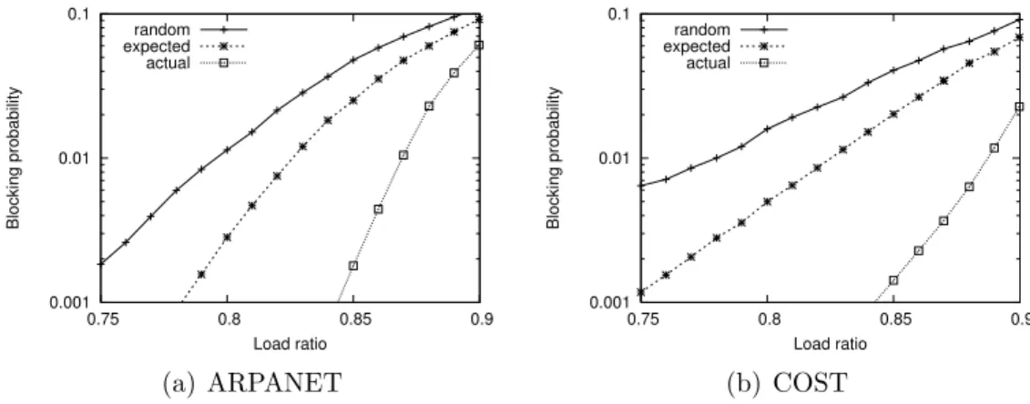
This section quantitatively measures the benefits of basic dimensioning and incremental dimensioning techniques for actual, random, and expected traffic patterns in the traffic evolution model.
3.4.1 Simulation Setup
The simulator was built according to the network model described in Sec-tion 2.5. In my simulaSec-tion, the arrival rate of each connecSec-tion ranges from 1 to 10. By default, the selection distribution is uniform. Each connection requests one wavelength channel and has the same departure rate. The de-parture rate is determined by the network load, which is the product of the projected departure rate and the load ratio. The setup is statistically equiv-alent to the general traffic model with variable departure rate and capacity demands. I use three well-known networks for the experiments: NJ LATA, COST 239, and ARPANET (Figure 2.6). The total capacity stays the same for each network in all experiments, with an average of 120 wavelengths per link. Network performance does vary with changes in the average link capac-ity. The current setting provides a interesting range of operating load with reasonable simulation effort.
The dimensioning process BAL(T, u, ξ) is defined by Algorithm 3.1.
RUN(T, B, X, β, l) is defined as a simulated routing process with a choice
of an online routing algorithm β ∈ {SP F, W SP, LRW, CAR}, given traffic matrixT and capacity resource (B, X). SPF, WSP, and LRW are introduced in Chapter 2. An optimized dynamic routing algorithm, congestion aware routing (CAR) (which is introduced in Chapter 4), is also applied here. The blocking probability is sampled by averaging 5000 arrivals in steady state.
0.001 0.01 0.1 0.75 0.8 0.85 0.9 Blocking probability Load ratio MEAN var u/l
SD var u SD var l (a) ARPANET 0.001 0.01 0.1 0.75 0.8 0.85 0.9 Blocking probability Load ratio MEAN var u/l
SD var u SD var l
(b) COST
Figure 3.2: Comparing projected load scaling (var u with l =u, ǫ= 0) and offered load scaling (var l with u= 0.85, ǫ= 0) using Algorithm 3.4 and SPF routing.
3.4.2 Traffic Load Scaling
I first study performance when complete traffic pattern information is known at the dimensioning stage. The normalized future traffic matrix is the same as the projected traffic matrix. There are two kinds of load scaling scenarios, projected load scaling and offered load scaling (Algorithm 3.4). In projected load scaling, the ratio of incremental dimensioninguvaries with the projected load ratio, as specified by Equation (3.2). The offered loadlis the same as the projected load u. As u increases, the portion of overdimensioned capacity on each link decreases proportionally. In offered load scaling, the network is assumed to be dimensioned at a fixed projected load ratio (u = 0.85, and l varies from 0.75 to 0.9). However, the real traffic offered scales over the projected traffic with the same ratio defined by Equation (3.5). The results of both experiments are averaged across m = 100 random projected traffic matrices. For both load scaling cases, MEAN results are identical because offered load scaling is the same as implicit MEAN over-dimensioning. Figure 3.2 shows that the SD approach improves relative to MEAN on both ARPANET and COST. The performance results of projected load scaling and offered load scaling are the same in the studied load range.