A hybrid approach for alarm verification using stream processing, machine learning and text analytics

A Hybrid Approach for Alarm Verification using Stream

Processing, Machine Learning and Text Analytics

Ana Sima

Zurich University of Applied Sciences

Winterthur, Switzerland [email protected]

Kurt Stockinger

Zurich University of Applied Sciences

Winterthur, Switzerland [email protected]

Katrin Affolter

Zurich University of Applied Sciences

Winterthur, Switzerland [email protected]

Martin Braschler

Zurich University of Applied Sciences Winterthur, Switzerland [email protected]

Peter Monte

Lukas Kaiser

ABSTRACT

False alarms triggered by security sensors incur high costs for all parties involved. According to police reports, a large majority of alarms are false. Recent advances in machine learning can enable automatically classifying alarms. However, building a scalable alarm verification system is a challenge, since the system needs to: (1) process thousands of alarms in real-time, (2) classify false alarms with high accuracy and (3) perform historic data analysis to enable better insights into the results for human operators. This requires a mix of machine learning, stream and batch processing – technologies which are typically optimized independently. We

combine all three into a single, real-world application.

This paper describes the implementation and evaluation of an alarm verification system we developed jointly with Sitasys, the market leader in alarm transmission in central Europe. Our sys-tem can process around 30K alarms per second with a verification accuracy of above 90%.

1

INTRODUCTION

False alarms triggered by sensors of alarm systems pose a signifi-cant challenge due to the high costs they incur for all involved parties. On the one hand, false alarms waste expensive police, medical and firefighter resources. On the other hand, Alarm Re-ceiving Centers (ARCs) cannot efficiently prioritise important alarms, because they are overwhelmed with false ones. According to police reports, a large majority of alarms prove to be false [34]. This is often attributed to technical errors, installation errors or user errors. As a consequence, owners of alarm systems end up switching their systems off to avoid the risk of paying for intervention forces deployed as a response to a false alarm.

From a technical perspective, false alarm verification is very challenging, since it requires the combination of three tradition-ally separate fields, namely stream processing, batch processing and machine learning. Depending on the data sources used for verification, both structured data (originating from the physical security sensors) and unstructured (originating from external sources, such as social media or police news feeds, available in free-text format) should be integrated. Recently, stream and batch processing have been integrated into combined systems such as

© 2018 Copyright held by the owner/author(s). Published in Proceedings of the 21st InternationalConference on Extending Database Technology (EDBT), March 26-29, 2018, ISBN 978-3-89318-078-3 on OpenProceedings.org.

Distribution of this paper is permitted under the terms of the Creative Commons license CC-by-nc-nd 4.0.

Flink [7] or Apache Structured Streaming [44]. However, adding machine learning, unstructured data and a real use-case to the equation makes the problem much harder. Machine learning has proven successful in a wide range of classification and anomaly detection tasks [26]. In particular, a classification model can be trained in order to compute the likelihood that a new alarm is either true or false, based on the history of alarms previously received in the system. Such algorithms have the potential to significantly reduce costs involved by false alarms, by enabling ARCs to focus on the alarms that are most likely true, while reducing the priority and the resources allocated for alarms that are likely false.

In this paper we present our experience in building an end-to-end alarm verification system that combines stream processing, batch processing and machine learning on both structured and unstructured data in an industrial setting. We use state-of-the-art Big Data technology such as Apache Kafka [21], MongoDB [33] and Apache Spark [38]. We show that our models can classify false alarms with over 90% accuracy and can scale up to 30K alarms per second including historical analysis using real alarm data from our industrial partner. Furthermore, we show that our models can be adapted with minimal effort and achieve good performance for similar use cases. For example, we use the same algorithms to train a new model from the history of fire incidents recorded by the cities of London and San Francisco.

The main contributions of this paper are:

• We present an end-to-end application that combines stream processing, batch processing and machine learning in or-der to uncover false alarms in an industrial setting. Using a dataset of 350K real alarms from alarm sensors deployed in production, we evaluate 4 machine learning algorithms and show that the best 2 algorithms (random forest and deep neural networks) can classify alarms with over 90% accuracy. This is, to our knowledge, the first study to show the applicability of machine learning techniques for false alarm reduction in the field of physical security, using real data collected from alarm sensors used in production.

• We show that a simple set of generic alarm features (loca-tion, time, property type) can be used for similar use cases. By reusing the exact same algorithms implemented for our industrial use case, we yield a verification accuracy of above 80% for the additional datasets from the cities of London and San Francisco.

•We discuss how to extend the approach to include a-priori risk factors extracted from external sources, such as news articles and social media postings, that potentially cover incidents related to alarms ("hybrid approach"). These sources usually provide unstructured, free-text data. In our prototype implementation, we focus on reports about fire and intrusion incidents. Even though we had only limited external data available, we increased the accuracy of our classifications from a baseline of 86.56% for the subset of fire and intrusion alarms to 87.56% when including the a-priori risk in the machine learning model.

The rest of this paper is organized as follows: We introduce Related Work in Section 2. In Section 3 we present the indus-trial use case for alarm management. We discuss the architecture as well as the design of our system in Section 4. We describe our experiments with various machine learning algorithms as well as end-to-end performance results based on stream process-ing, batch processing and machine learning in Section 5. Finally, we present an extensive list of lessons learned in Section 6 and conclude in Section 7.

2

RELATED WORK

2.1

Stream Processing

Stream and continuous event processing for real-time analyt-ics has been a major topic of the database community for more than a decade with Aurora [9] being one of the pioneers. Other popular systems are Gigascope [13], Esper [16] or Stream Base [40]. Common to these systems is that they provide a declarative query language based on SQL to process data streams. The advan-tage of these systems is that end users can formulate analytics queries using the expressiveness of SQL rather than learning new APIs. Moreover, since SQL is declarative, the end-users need not care of how they would optimize the system performance since the stream systems can apply query optimization techniques by understanding the query patterns.

Common to all these systems is that they are highly specialized for one particular functionality, namely stream processing with short time windows. However, they are inadequate for combined stream and batch processing since they only focus on stream processing.

2.2

Real-time Data Warehousing

Typical data warehouses of large enterprises are used for report-ing, analytical and predictive purposes. In order to optimize query performance, these systems organize data in a star schema [10]. Moreover, data is usually ingested on a daily or subdaily basis. Common to all traditional data warehouses is that they are very efficient for processing historical data but not particularly well suited for processing streams of data.

In order to overcome these problems, recently so-called data stream warehouses have been proposed to handle both big and fast amounts of data within one single system. In other words, the idea is to use one, combined system for stream and historical data analytics. Examples of such systems include Borealis [1], DataDepot [17], DejaVu [14], Moira [6] or TruViso [24].

The advantage of these systems over streaming-only systems is that they can handle combined workloads of both stream and batch processing.

2.3

Combined Stream and Batch Processing

As part of our previous work we have used bitmap indexes to enable stream and batch processing in TelegraphCQ [35]. We have demonstrated the approach for analyzing a large set of network traffic data.

To tackle the problem of combined stream and historical data analytics for more recent Big Data systems, the Lambda archi-tecture [31] was introduced that currently sets the standard in system design for building big data real-time analytics environ-ments. It is trying to provide a solution to compensate latency and waiting time when accessing and analyzing batch processed data through the availability of real-time data streams. However, criticism on the Lambda architecture revolves around the oper-ational complexity of systems implementing this architecture. This does not only include operations of the systems but espe-cially also implementing and maintaining an efficient code base for the two different data processing approaches - stream and batch processing - used in systems built according to the Lambda architecture.

Real-time processing for NoSQL systems has recently been introduced in Muppet [25], SCALLA [29] and Spark Streaming [44]. In particular, structured streaming seems very promising. Another system that provides both stream and batch processing is Apache Flink [7]. However, it is still difficult to smoothly in-tegrate different technologies to develop a system for complex scenarios that can leverage existing legacy systems. A more re-cent reflection on main memory vs. stream systems can be found in [23].

2.4

Machine Learning for Anomaly Detection

Machine learning has been widely used for classification and anomaly detection. The research closest to ours has been done in intrusion detection systems in the field of computer and network security [26]. Subsequently, in order to make these systems usable in practice, a lot of work has focused around means to reduce their false positives [27], [4], [12]. The recent shift of the alarm industry towards IoT and smart connected sensors has opened the path for applying the same algorithms in a relatively new context, namely that of physical security, which is our focus in this paper. There is to-date surprisingly little published data on the effectiveness of these techniques for physical IP-connected alarm systems.

Most of the related work published either in research papers or in industrial patents aims at reducing false alarms by means of verification through a secondary channel - e.g. a video camera or additional sensors, such as temperature, shock or vibration sensors. In [30], an intelligent home security system based on the ZigBee protocol is presented. The system detects false alarms by means of image processing from surveillance cameras. However, we do not rely on any other information apart from alarm device properties, the type of supervised premise, location and time.

Similarly, a patent issued by Honeywell AG presents a system that reduces false alarms in a home security system by using information provided by additional sensors, such as an acous-tic glass break sensor, shock sensor and vibration sensor [3]. More recently, Honeywell extended their systems with a video-verification step to reduce the number of false alarms [19]. In contrast, our approach has the advantage of being more generic, given that it relies only on information provided by basic sensors and a model trained offline (from the history of alarms received

Figure 1: Alarm System Architecture. ARC = Alarm Re-ceiving Center.

from these same sensors), even in the lack of more contextual information (camera images, weather sensors etc).

An interesting approach is presented in [32], where the most suitable machine learning algorithm is chosen adaptively based on the performance of the currently used one - this could be an interesting path for future work in our system, as we have already implemented 4 machine learning pipelines, therefore we would only require the logic to adaptively choose among these at run-time. Another angle to consider would be a majority vote among the different classifiers, providing the overall verification and probability as an aggregate of the information provided by all 4 classifiers.

In a recent publication, Spark Streaming [44] and Apache Kafka [21] were used to detect anomalies in Big Data streams by applying various metrics based on entropy theory and Pearson correlation [36]. In our project we partially build on these results. Our initial machine learning experiments showed promising results [37].

3

ALARM VERIFICATION USE CASE

In a typical security installation, transmitting an alarm originat-ing from a sensor (e.g. motion or smoke detector) to a security organization involves a chain of equipment and people. A simpli-fied view of this setup is shown in Figure 1. An alarm triggered at a supervised premise (a home or enterprise) will reach the se-curity organization (also called Alarm Receiving Center - ARC), where the alarm is handled by one of multiple operators who take predefined actions based on the so called action plan which was previously elaborated together with the customer. This usu-ally involves trying to contact the customer by phone to verify the alarm. This is an important step because more than 90% of all alarms are false positives [34]. If the operator is not able to reach out to the customer or the alarm was verified, he sends out intervention personnel (police, ambulance or firefighters) to go on-site.

The high amount of false alarms makes alarm handling costly. Certas AG, one of the major companies in the alarm monitoring market, processes nearly 5 million alarms and over 2 million phone calls a year, as they report in the Alarm Management Sym-posium in 2017 [11]. Our industrial partner, Sitasys, operates a platform that connects hundreds of such monitoring centers. To-day, a large number of messages are generated from a relatively small amount of sources (like fire sensors or motion detectors).

With the advent of Smart Homes and IoT technologies, the num-ber of sensors and therewith the numnum-ber of alarms is expected to increase drastically. Meanwhile the demand for security also in-creases. The security industry in Austria, for example, has grown almost 45% between 2010 and 2016 (as indicated in the yearly security book 2017 published by VSO [42]). With these trends, the monitoring centers risk to get flooded with alarm messages. Keeping in mind that the rate of false alarms is above 90%, it becomes clear that there is a need for improvement.

Uncovering false alarms through machine learning is challeng-ing, since there may not even be a clear definition on whether an alarm is worthy of investigation or not, thus rendering a 100% accuracy a hypothetical goal. However, by changing the pro-cess of alarm handling, there might be a way to use predictive modelling in a safe way in order to reduce costs significantly. The way this could be achieved is to transfer the verification of the alarm partly to the customer. The idea is to transmit alarms with a high probability of being false positives to the customer’s mobile phone first. The customer can then decide within a time window whether the alarm is real or false and whether it should be sent to the alarm receiving center. Only alarms with a high probability of being true (and those for which a timely answer could not be received directly from the customer), are forwarded to the monitoring center, which can then send out intervention personnel.

With this approach, the number of alarms arriving at the monitoring center decreases, while the handling of the particular alarm becomes more effective, since the manual verification can be omitted. With this self-monitoring solution, the customer can actively take part in the alarm processing chain, which will decrease the workload at the monitoring center and consequently potential errors caused by overwhelmed operators.

Furthermore, the probability for true and false alarms can be used by the monitoring center in order to effectively prioritize alarms. This is especially helpful in the case of large events, which generate a spike of messages that need to be processed fast. An effective prioritization of alarms allows a more effective use of intervention personnel. This ultimately benefits the customer as well, because it reduces the fees he has to pay if the police or fire brigades respond to false alarms repeatedly.

The solution envisioned by Sitasys involves an online portal called "My Security Center". Using "My Security Center" the cus-tomer can configure the threshold for the probability of alarms being classified as true. The customer thus decides which alarms should be sent to the monitoring center and which should be sent to his mobile phone first. He can also decide not to send technical alarms, like connection interruptions, to the monitoring station at all. Based on his settings, the alarm handing can be offered for about 40% of the price that is currently common in the market – without any sacrifice concerning security. Since "My Security Center" allows dynamic changes of the rules how and where alarms are being transmitted, it will also allow the offering of more custom tailored services.

4

SYSTEM DESIGN

In this section we motivate the main workflow, the system ar-chitecture for our alarm verification application and discuss our design choices.

Figure 2: System design consisting of four components: (1) Stream Processing, (2) Batch Processing (Alarm History), (3) Machine Learning (Verification Service) and (4) Hybrid Approach (Incident History).

Figure 3: Workflow diagram.

4.1

Workflow

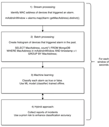
The workflow for alarm verification, shown in Figure 3, consisting of stream processing, batch processing and machine learning, can be characterized as follows.

The stream processing part identifies all devices that trigger an alarm within a certain observation period (the streaming window). As part of the batch processing part, all devices that triggered an alarm are analyzed in more detail by producing a histogram of the number of alarms starting from a specific time

t. Finally, for all the new alarms in the given time window, a machine learning algorithm verifies whether the alarm is true or false, based on a classifier trained periodically offline (for example, once per day during idle periods, such as after midnight).

Figure 4: System Architecture and Process Flow

4.2

System Architecture

An overview of the system we developed for handling the above mentioned workflow is shown in Figure 2. The four main com-ponents we developed are:

(1) Streaming Component. This component is responsible for transmitting and receiving alarms. The simplified format of an alarm sent by a Sitasys sensor through a Kafka stream is shown on the left hand-side of Figure 4. We chose Apache Kafka [21] for this component as it is the state-of-the-art distributed streaming platform, highly scalable and also easy to integrate with Spark. We coupled Spark with Kafka through Direct Dstreams [44], which offers exactly-once semantics "out-of-the-box". This is crucial in our case in order to ensure that we neither miss an alarm, nor process the same one multiple times. For more details refer to [22].

(2) Batch Component (Alarm History). This component is re-sponsible for long-term storage of alarms and for doing batch analytics on the history of alarms. For this com-ponent we chose to use MongoDB [33], both because of its flexibility (we can store alarms directly as JSON-like documents and query by fields, such as by location of the alarm in order to compute a histogram) and because of its scalability.

(3) Machine Learning Component (Verification Service). The reception of a new alarm through the stream immedi-ately triggers the computation of a classification (true/false alarm) and the associated probability (confidence), based on a machine learning model trained offline. The verifica-tions will be used by the Alarm Receiving Centers in order to prioritize incidents where an intervention (police or fire department) is highly likely to be required. We chose to implement this component using Apache Spark, first because it is easy to scale-out when required - for exam-ple, if more customers install alarm systems - and second, because of its fault tolerance guarantees. Coupling Kafka with Spark results in an exactly-once semantics streaming application.

(4) Hybrid Approach (Incident History). For the hybrid ap-proach we collect reports about fire and intrusion inci-dents in Switzerland. The inciinci-dents are reported as textual data, for example in RSS feeds, Twitter messages or web-pages (see Figure 5). The goal is to use this historical data in order to calculate an a-priori risk factor per each lo-cation (village or city in Switzerland) and incorporate it in the machine learning model. Our pipeline collects as many reports as possible and then filters those pertaining to relevant topics (fire and intrusion), based on a set of keywords defined in the pipeline. Each incident report is then annotated with a time and location, extracted directly

Figure 5: Schema of the incidents history pipeline. In a first step, reports from different sources, such as Twitter, RSS feeds and web pages are collected. Next, reports re-lated to relevant topics (e.g. fire, intrusion) are selected (fil-tered). The remaining relevant reports are annotated with a date, a location and a language and saved in MongoDB.

from the textual data or from the metadata (if available). Finally, similar to the alarm history, we store the incident history in MongoDB. The a-priori risk factors are defined as the number of incidents per capita on location level.

4.3

Reflection on Design Choices

One of the major design choices was the architecture and technol-ogy used for streaming processing, batch processing and machine learning. For stream processing the main options available were Apache Storm [39], Apache Kafka and Apache Spark Streaming [44]. We have decided for the combination of Apache Kafka and Spark Streaming due to the good integration and the scalability of both systems. Even though Storm allows topologic modelling of streaming tasks, we decided against it since our application does not have a complex dependency between tasks.

In order to combine stream and batch processing, the design choices would be either the more traditional Hadoop stack for batch processing combined with Storm for streaming processing, or the more recent, in-memory, Apache Spark technology. We have chosen the latter due to its tighter integration of function-ality (stream and batch processing as well as machine learning available in a single framework). This was an important advan-tage for our industry partner Sitays, in order to decrease the complexity of the overall system architecture, as well as to re-duce maintenance costs and required skills of their workforce.

At the start of our project, Spark Structured Streaming was marked experimental, therefore not yet production ready, hence we decided against it. Moreover, our industry partner has a large collection of alarm data stored in MongoDB which should be leveraged. After analyzing the integration of Spark with Mon-goDB, we decided for this design option since it allowed us to re-use technology already existing at our industrial partner and

to effectively combine it with state-of-the art stream process-ing. Moreover, MongoDB is flexible to schema changes, which makes it a better option for long-term storage than a traditional Relational Database, given that in our use case the structure of an alarm differs across sensor types and even across software updates. Using MongoDB allowed our industry partner to easily ingest data from new alarm installations, even when the structure of the new alarm data did not match the structure from previous installations. In our experiments we achieved satisfying scala-bility results of MongoDB queries for large datasets. For more details see Section 5.

Using Spark ML for machine learning was a natural choice since it is readily integrated within the Spark technology stack. However, since Spark ML did not provide deep learning algo-rithms at the start of our project, we used various other deep learning frameworks such as DeepLearning4J [15] as well as Theano [41] and Lasagne [28].

5

EVALUATION

In this section we first describe the alarm datasets we used for our experiments, namely from Sitasys, as well as from the cities of London and San Francisco. Next, we describe the incidents dataset we used for the hybrid approach to enrich the Sitasys alarm dataset. This is followed by a description of our machine learning experiments in order to classify false alarms and a description of our experiments using the hybrid approach in order to improve the machine learning pipeline. Finally, we present the end-to-end evaluation of our system, which includes stream processing, batch progressing, as well as machine learning. Our results show that using production data we can process 30K alarms per second with an accuracy of above 90%.

5.1

Alarm Datasets

In order to build and evaluate a model for false alarm verification, we started by analyzing the alarm data provided by our industrial partner, Sitasys. This data is presented in Section 5.1.1. First, we selected the set of features best suited for verification. We describe this in Section 5.3. Then, in order to evaluate how well we can extrapolate using this set of features for similar use cases, but also to see how well our algorithms scale, we looked for larger datasets available online. We identified two candidates, namely the London Fire Brigade Data and the San Francisco Fire Department Data. The most relevant features from all 3 datasets are shown in Table 1. In the next sections we describe each dataset in more detail.

5.1.1 Sitasys Production Data.Real alarm data from October 2015 to April 2016 was collected and anonymized by our indus-trial partner Sitasys, gathering a total of 350K alarms in roughly equal proportions of true and false alarms. The main types of in-formation provided are location (ZIP code), device address (MAC and IP address), timestamp, alarm duration, type of incident (fire, intrusion, etc.) and a few other sensor-specific information (type of sensor, software version, etc). The ObjectType feature classifies the type of supervised premise the alarm originates from: indus-trial, residential etc. The location information was anonymized (hashed) for privacy reasons. One important challenge we faced when using this data is the lack of real labels (i.e. indications about true and false alarms). These could not be provided to us in due time from the Alarm Receiving Centers that register them. However, in collaboration with Sitasys we have defined a heuristic to infer the labels, which is to consider the duration of

Dataset Location Time Type of Location Incident Type Label Sitasys ZIP code Timestamp ObjectType Alarm Type Alarm Duration London ZIP code Date/TimeOfCall PropertyType PropertyCategory Incident Group San Francisco Zip code Of Incident ReceivedDtTm - Call Type Call Final Disposition

Table 1: Features of the three data sets

Figure 6: London Fire Brigade Statistics

the alarm as a threshold - the more quickly the alarm was reset after being triggered, the higher the likelihood that the alarm was false, given that the customer was able to reset it in a short period of time. We chose several different values for the alarm reset duration threshold between 1 and 10 minutes. We used 50% of the alarms for training (roughly equal amount of true and false alarms) and the remaining 50% for testing. Moreover, we were interested in the response time for an incoming alarm on a data stream, therefore we also simulated a stream of new alarms from the testing data and tested the performance of our verification system. Details are given in Sections 5.3 and 5.5.

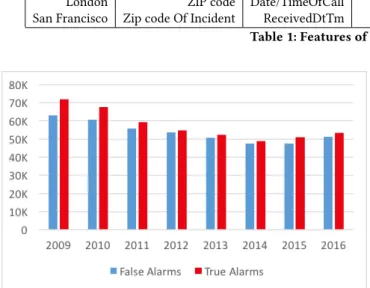
5.1.2 London Fire Brigade Data. The London Fire Brigade (LFB) is the busiest fire and rescue service in the United Kingdom and one of the largest firefighting and rescue organizations in the world. We used the open data of every incident reported since January 2009, available online1. The dataset provides information about the location, time and type of incident for all records.

Figure 6 shows the high-level statistics of incident groups between 2009 and 2016, as well as the ratio of false vs. true alarms recorded. In total, 885K incidents were recorded, out of which 430K (48%) were false. This dataset is therefore very convenient to use for our classification algorithms, because the true and false classes are almost equally balanced, which makes it suitable even for algorithms that are very sensitive to unbalanced data (e.g. Random Forest).

This dataset is useful for two purposes: first, it allows us to test hypotheses on a coarser time-scale, since the incidents are recorded from 2009 until today, meaning that for example we can try to draw statistics and make verifications based on the days of the year with peaks of incidents. Second, it serves as a scalability test as the number of incidents is twice as larger as those provided by our industrial partner.

1_{https://data.london.gov.uk/dataset/london-fire-brigade-incident-records}

5.1.3 San Francisco Fire Department Open Data.In an attempt to extend our study, we also considered the San Francisco Fire De-partment Dataset (available online2), which contains 4.3 million incidents from the city of San Francisco from the year 2000 until today. We found that, in contrast to the London Fire Brigade Data, the quality of the San Francisco dataset is lower, given that more than half of the records (2.5 million) are not properly labeled, the Call Final Disposition - which denotes the final classification of the incident - marked "other". Only 105K are explicitly labeled as "No Merit" (false alarm), i.e. less than our production data from Sitasys from 2015 and 2016 only. Moreover, as shown in Table 1, there is no entry in the dataset that indicates the type of property, which in our study of the Sitasys alarms proved to be an impor-tant feature for the classifier. An added problem is the diversity of the types of incidents recorded. For example, more than half of the entries are medical incidents, which are not present at all in the other two datasets. Around 1 million incidents are alarms and fire incidents and only a small fraction of these are properly labeled.

All in all, in our study we could only consider incidents of type "alarm" and "fire" that have a proper label indicating either true or false alarm. Unfortunately, this only results in around 12K incidents, much less than we initially expected. We report results from this small subset in the next section. Finally, we note that we have tried our classification algorithms againstallproperly labeled incidents (including medical, hazards etc) but for this purpose we did not obtain meaningful results - only around 53% accuracy.

5.2

Incidents Dataset

This dataset is a collection of reports about real fire and intru-sion incidents, gathered from online resources, such as RSS feeds, Twitter or relevant web pages (police, fire brigades etc.). This ex-ternal data is used in order to enrich the knowledge base provided by theSitasys Production Data. In particular, we annotate alarms with an a-priori risk factor, based on their location. Since the

Sitasys Production Dataonly consists of data from Switzerland, we focus on collecting reports about Swiss incidents. For exam-ple, we collected messages related to incidents from 50 different Twitter accounts (cantonal police, fire brigade departments and others) from January 2015 until end of October 2017. Our pipeline checks, for each message, whether it contains information about intrusions or fire (see Figure 5). Next, it identifies the language, the date and the location of the incident, either from the meta-data (if available) or directly from the textual meta-data (the message). However, since the metadata does not contain information about ZIP codes, the granularity of each location is either a city or a village. In turn, the granularity of our alarm data set is slightly more detailed, namely, at the level of ZIP codes. For example, some larger cities, such as Basel and Zurich, have multiple ZIP codes for different districts of the city. Since the incidents dataset does not have the same level of granularity as the alarms dataset,

2_{https://data.sfgov.org/Public-Safety/Fire-Department-Calls-for-Service/}

nuek-vuh3/data

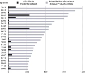
Figure 7: Discrepancy between the amount of incidents and amount of true fire and intrusion alarms in the two data sets.

Figure 8: Screenshot of the security map with focus on Zurich (Switzerland). Red areas imply a higher risk level.

we can only approximate an aggregated risk over all districts of a large city with several ZIP codes (see Table 2).

The dataset contains 5,056 descriptions of incidents, out of which 2,743 are in German, 1,516 in French and 797 in English. The corresponding incidents are located in 1,027 distinct cities and villages of Switzerland, covering around 1/4 of all cities and villages in Switzerland. The discrepancy between the number of incidents in the dataset and true fire and intrusion alarms in theSitasys Production Datais shown in Figure 7. For example, the first entry in Figure 6 shows the number of true fire and intrusion alarms for the location with ZIP code 3013 provided from theSitasys Production Data(lower bar shown in light gray). However, the number of reports about fire and intrusion incidents is significantly smaller (upper bar shown in black).

Finally, we use the incidents dataset to build and display a security map of Switzerland, shown here in Figure 8. The fig-ure shows the risk of different areas in the canton of Zurich, Switzerland. Green areas indicate safe regions, whereas yellow indicate medium-risk and finally, red implies higher risk. For a detailed discussion on the calculations of the risk levels we refer to Section 5.4.

#-true-alarms #-incidents ZIP codes Basel intrusion fire intrusion fire

4001 43 3 [unknown] 4051 142 3 [unknown] 4057 304 0 [unknown] 4058 0 55 [unknown] Total for city of Basel 489 61 10 464 Table 2: Divergence between the number of true alarms in different districts in Basel (Switzerland) in the Sitasys Production Data and the number of incidents collected in the Incident Data. The Incidents Data only contains loca-tion informaloca-tion at a coarser granularity (per city / village) than the Sitasys alarm data (per ZIP code).

5.3

Machine Learning

We chose 4 of the most commonly used algorithms for ma-chine learning: Random Forest, Support Vector Mama-chine, Logistic Regression and Deep Neural Networks (DNN). For the first 3 we used the readily available implementations from Spark ML, whereas for DNNs we developed an application using DeepLearn-ing4J [15] as well as Theano [41] and Lasagne [28].

For feature selection we first evaluated which of the alarm fields best separate true from false alarms. We used the Pear-son correlation inspired by [36] to find dependencies between features and labels as well as dependencies among features. In addition, we ran a grid search for each algorithm, varying the features used to train the models, and finally selected the follow-ing most promisfollow-ing features: location (for privacy reasons we only received hashed location information), day of week, hour of day, alarm type and property type.

Although in our experimental evaluation we only take into account accuracy in terms of number of correct verifications, we note here that, given that our main use case is a decision support system for human operators in the Alarm Receiving Centers, not only is the verification important, but also the probability (confidence) associated with it, as the human operator will likely take a decision according to this metric rather than just the verification.

For our experiments we used the following hardware setup:

• For initial experiments using a single Producer, single Consumer workflow, described in Section 5.5, we used two Intel Xeon E5-2620 machines at 2.4 GHz with 8 GB RAM.

• For multi-node Spark experiments we used a cluster of 4 Intel Xeon E5-2640 CPUs at 2.5 GHz with 16 GB of RAM each.

• For the DNN experiments we used 1 Intel Xeon E5-2650 with 1 Titan X GPU.

5.3.1 Accuracy.As our main use case is to verify false alarms based on the alarm data from our industrial partner, we focused on extracting the features that best separate true from false alarms in the Sitasys dataset. We then investigated how well the equiva-lent set of features in the open data sets from London and San Francisco can be used to verify false alarms. We show in the next subsections that our approach can be easily transfered to these 2 similar use cases with good accuracy results.

5.3.2 Parameter Tuning. The first important parameter we investigated for the Sitasys alarm dataset was the threshold for

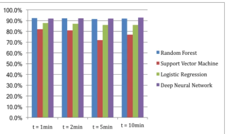
Figure 9: Verification Accuracy vs.∆t (Sitasys Dataset)

the alarm duration. This parameter is used as a heuristic to deter-mine whether the alarm is true or false. For example, when using a threshold of 1 minute, all alarms with a duration smaller than 1 minute are considered false. The intuition is that an alarm that was reset (turned off) within a very short time is likely false (the owner immediately shut it off). In order to evaluate the effective-ness of our machine learning approach, we experimented with various values for delta t ranging between 1 and 10 minutes. The goals of our evaluation were as follows: (1) Evaluate the accu-racy of four different machine learning algorithms. (2) Study the impact of various deltas t on the verification accuracy. The idea was to show that the results are stable with respect to changes in the choice of delta t. The results are shown in Figure 9. We can see that on average the best classification quality among all algorithms is achieved with the smallest threshold, of 1 minute, and that moreover in all cases Random Forest and Deep Neural Networks achieve the best performance, of over 90% accuracy, independent of the choice of delta t, which means the accuracy results are stable across changes in the choice of this parameter. Next, the selection of hyper parameters for each of the learning algorithms (e.g. architecture of neural network) was essential for the verification accuracy. We used grid search to tune the hyper parameters. Tables 3, 4, 5, 6 and 7 show the best ones for each of the 4 algorithms we tested.

Parameter Value Maximum depth of a tree 30 Number of trees to train 50 Table 3: Parameters for Random Forest

Parameter Value Maximum number of iterations 2,000 Step size 1.0 Mini batch fraction 0.2 Regularization parameter 1e-2 Kernel Linear Update Function Squared L2 Table 4: Parameters for Support Vector Machine

5.3.3 Training Time.One important factor we investigated to ensure that our prototype is usable in practice is the train-ing time. Essentially, this determines how fast we are able to

Parameter Value Maximum number of iterations 500 Convergence tolerance of iterations 1e-6 Table 5: Parameters for Logistic Regression

Parameter Value Maximum number of epochs 10,000 Mini batch size 200 Loss function Cross Entropy Update function Nesterov Momentum Learning rate 0.1

Momentum 0.9

Table 6: Parameters for Deep Neural Network

Layer #Nodes Type Activation Function Input 803 Nodes

Hidden 1 50 Nodes Fully connected ReLU Hidden 2 2 Nodes Fully connected ReLU Output 2 Nodes Fully connected Softmax Table 7: Architecture of Deep Neural Network

rebuild our models, a step that is required periodically (ideally, upon reception of a large enough number of new events, for example once per day). Table 8 shows the training times for our classification algorithms, using the 3 datasets: Sitasys, London Fire Brigade (LFB) and San Francisco Fire Department (SF). The short training time for the San Francisco dataset is explained by the fact that we can only use around 12K incidents properly labeled from the alarm and fire categories. Another observation is that for all the datasets, the smallest training time is required for Logistic Regression, while Deep Neural Networks take much longer to train. Moreover, we use the One Hot Encoding for this algorithm, which means we end up with twice as many input features (around 800) for the Sitasys dataset than for the oth-ers (around 300), given that we also use some sensor-specific categorical features in the case of Sitasys (each of the values of these attributes becomes a separate feature when using One Hot Encoding).

Algorithm Sitays LFB SF Random Forest 600 1200 75 Support Vector Machine 200 480 20 Logistic Regression 100 60 10 Deep Neural Network 5100 2460 60

Table 8: Training Time [sec] for Machine Learning Algo-rithms

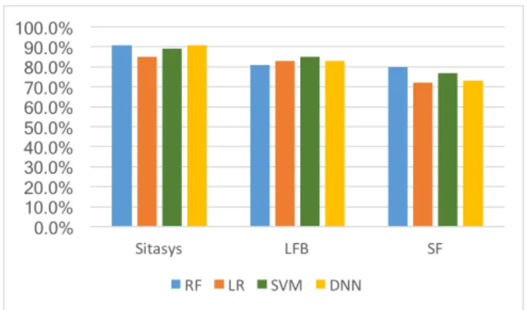
5.3.4 Accuracy Results.Figure 10 presents a comparison of the accuracy obtained for the 3 datasets we tested. We can see that the best results are obtained for the Sitasys dataset with a classification accuracy of up to 92% for Random Forest. The promising results can be explained by the fact that, apart from the generic features (Location, Property Type, DayOf Week and HourOfDay), the Sitasys dataset contains a few other features that can identify technical faults more easily (sensor-specific in-formation), which allows the algorithms to better classify false alarms. By contrast, for the LFB and SF datasets we could only use

Figure 10: Verification accuracy comparison using four different machine learning algorithms for three Sitasys, London Fire Brigade (LFB) and San Francisco Fire Depart-ment (SF) Datasets. RF = Random Forest, LR = Logistic Regression, SVM = Support Vector Machine, DNN = Deep Neural Network

the generic features. However, it is interesting to note that this still results in fairly good accuracy, of around 85%, for the LFB dataset (best result is obtained for the Support Vector Machine) and 80% for the SF dataset (Random Forest). As mentioned pre-viously, the San Francisco dataset does not contain information regarding the type of property an alarm originates from, which could explain the lower accuracy. Furthermore, the volume of the training data we could select from the SF dataset is generally too low (only around 12K alarms).

Another interesting result is that, although there are some differences among the accuracy results for the 4 algorithms we tested, they are never higher than 5%. This is encouraging for two reasons. First, because some algorithms require less training time and less resources to run (Logistic Regression), therefore they could be chosen over the others in case response time is more crucial than accuracy. Second, because more generally this validates our approach, given that the good accuracy is not an artifact of a particular choice of machine learning algorithm, but rather a consequence of the feature selection, which accurately describes the problem we aim to solve. On the other hand, a 5% improvement in classification accuracy (from 85% to 90%) effectively means reducing the error rate by 50%, which means the best algorithms perform significantly better.

5.4

Hybrid Approach

For the hybrid approach we collected descriptions of fire and in-trusion incidents from different online resources, such as Twitter, RSS feeds, or web pages collected through a provider of web-based data feeds, webhose.io. Each incident is annotated with the time and location, extracted from the original message or web page. We use this information to calculate an a-priori risk factor for intrusion and fire alarms, based on the number of incidents that happened in a certain location (village or city), normalized by the population size. Next, we evaluate the impact of the in-clusion of a-priori risk factors on the accuracy of the machine learning model.

We chose three different ways to include the a-priori risk factors into our machine learning pipeline:

(1) absolute risk factor (2) normalized risk factor

(3) binary risk factor

(1) The absolute risk factor is calculated by dividing the num-ber of incidents found in various resources by the population in the annotated location. (2) The normalized risk factor has a range of 0 to 1, and is calculated asx′= x−min(x)

max(x)−min(x), wherexis

the absolute risk factor of a location. (3) The binary risk factors are either 0 or 1. The risk factor is 1, if the incident is in the most frequent 25% locations, otherwise the risk factor is 0.

Our efforts for the hybrid approach are still in the early stages, and the data we have collected so far is limited. As a consequence, for the evaluation we only use alarms with a ZIP code where we have corresponding reports about incidents. This reduces the number of alarms from about 350,000 to 130,958 (see Figure 7). As mentioned previously, the granularity of the alarm data is on ZIP code level, while the granularity of external reports about incident data is on city or village level. To analyze the influence of this discrepancy in granularity, we run additional experiments where we only select alarms about small cites or villages that have one ZIP code rather than multiple ones. This reduces the number of alarms from around 130,958 to 37,241 and further the number of incidents from 5,056 to 4,379 (see Table 9). Moreover, theSitasys Production Dataprovides more alarm types than fire and intrusion. Hence, we needed to filter only those alarms that are triggered due to fire or intrusion.

Table 9 shows the experimental results for alarm classification of four different scenarios (a-d) and three different a-priori risk factors, compared to a baseline approach. The baseline shows the alarm classification accuracy without a-priori risk factors (as reported in Section 5.3). The results are averaged over 10 runs for each experiment. In the scenario (a), using all locations and all alarms, we have around 130,958 alarms. This scenario only shows a small increase of 0.04% of the classification accuracy using the normalized risk factor. Scenario (b) uses all locations, but only the fire and intrusion alarms, which reduces the training data to 24,934 alarms. In this scenario, the results show that the absolute risk factor leads to an increase of 0.22% in accuracy compared to the baseline.

The scenarios (c) and (d) use only locations with a single ZIP code attached. Therefore we make sure that the a-priori risk fac-tor does not contribute wrong information to larger cities with multiple ZIP codes. Out of the total of 130,958 alarms, 37,241 refer to cities with single ZIP codes. This implies that around 2/3 of the alarms are located in larger cities. The results of scenario (c) show an improvement of 0.4% for the absolute risk factor, compared to the baseline. The normalized and binary risk factors also have a slight positive impact. Finally, scenario (d) uses only fire and intrusion alarms for cities with single ZIP codes. There-fore, the number of alarms is reduced to about 10,000 alarms. In this scenario, the impact of applying a-priori risk factors is the strongest, with an increase of 1% compared to the baseline.

Overall, the results obtained by including the external, unstruc-tured data are still preliminary. The scarcity of this data, coupled with an uneven distribution of the reported incidents makes it difficult to measure a significant impact. We still consider the re-sults promising, as they show a) that adding in potentially noisy textual information from third-party sources does not degrade the results even though we are using a limited set of collection and filtering approaches and b) that a small positive impact can al-ready be seen when focusing the analysis on the subset of alarms for which we have matching unstructured data.

all locations single ZIP code locations all types F/I alarms all types F/I alarms scenario (a) (b) (c) (d) baseline 89.35 85.73 87.16 86.56 ARF 89.29 85.95 87.56 87.45 NRF 89.39 85.67 87.41 87.56 BRF 89.31 85.79 87.51 87.48 #-incidents 5,056 4,379 #-alarms 130,958 24,934 37,241 10,036 Table 9: Accuracy of alarm classification using three dif-ferent a-priori risk factors and four scenarios: (a) all loca-tions, all alarm types, (b) all localoca-tions, only fire & intru-sion alarms, (c) single ZIP code locations, all alarm types and (d) single ZIP code locations, only fire & intrusion alarms. ARF = absolute risk factor, NRF = normalized risk factor, BRF = binary risk factor.

5.5

End-to-End Data Processing

Once we have trained and tested the machine learning algorithms, the next step was to build the end-to-end pipeline to integrate machine learning into stream and batch processing. In particu-lar, as soon as an alarm arrives, a machine learning algorithm classifies in real-time whether the alarm is true or false. In ad-dition, historical data analysis is performed on the sensors that triggered the new alarms. The goal of our experiments was to evaluate the maximum throughput of our system, identify poten-tial bottlenecks and to derive lessons learned from building such a production system.

5.5.1 Setup of Streaming System. In order to test the scal-ability of our prototype, we handcrafted a Producer application, which simulates a stream of new alarms. The stream is created by randomly selecting alarms from the test set (alarms from our production data, that have not been used for training the machine learning model) and writing them into Kafka, at a controlled rate (alarms per second). We aim to to evaluate the response time of our system, which runs as a Consumer application.

First, we are interested in measuring the maximum through-put (number of verified alarms per second) on the consumer side. We assume that the training phase has already been completed offline and the model is readily available for computing classfica-tions. Second, we must take into account the maximum latency (system response time) per alarm, as it is critical to ensure that a human operator in the Alarm Receiving Center can get a timely verification result. Currently we set the goal of responding in at most 10 seconds since the reception of the alarm at the ARC.

5.5.2 Identifying Bottlenecks.

Throughput of Producer-Consumer. With a setup as simple as just one producer and one consumer application (running each on a separate machine connected through a 1 GB Ethernet network), we were able to identify several bottlenecks in our system. First, our tests showed that both the producer and the consumer were processing events at an unexpectedly low rate (about 12K alarms produced per second, where one alarm is less than 1KB in size), even if Kafka benchmarks made us expect much higher throughputs. After further investigation we found that the bottleneck in both applications was in fact the serializer used for writing alarms into, and reading them from, the Kafka stream. At first, our implementation used the Jackson serializer, which turned out to be a poor choice for small objects [18], where the Gson serializer is more appropriate. We were surprised to find

Figure 11: Scalability Jackson vs Gson serializer

that just replacing this led to a 2x speedup in both applications. Figure 11 shows the results. We can see that by switching from the Jackson serializer to the Gson serializer the throughput of the producer more than doubled to about 25K alarms per second. On the consumer side, the increase was slightly less than double. This is due to the fact that the consumer has a higher computing load than the producer.

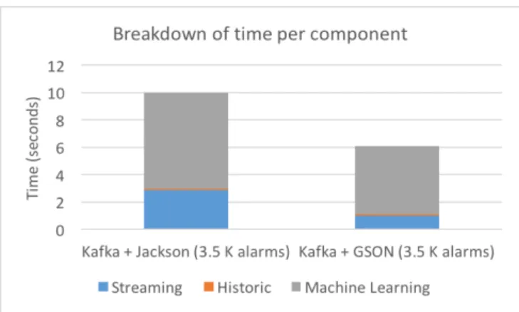
Detailed Analysis of Consumer. Next we analyzed the com-puting time of the consumer in more detail (Figure 12). In particu-lar we were interested in the time contribution of stream process-ing (Spark Streamprocess-ing), batch processprocess-ing (MongoDB query) and machine learning (Spark ML). The breakdown of time per compo-nent using a 10 second window of alarms shows that the majority of time is spent in the machine learning part (around 80% of the total time) to classify. We also notice that an insignificant fac-tor goes to the hisfac-toric component (retrieving the histogram of alarms originating from the same addresses as those in the time window). The remaining time goes to the streaming component: first, for deserializing alarms into the native Spark data format, RDDs (Resilient Distributed Datasets [43]), then for extracting all distinct addresses from the RDD etc.

Kafka Optimization. After this step, we further noticed that although our consumer machine has 8 cores, none of the compu-tations were parallelized, although Spark was configured to use all the cores on the local machine. After investigating this we found that by default, Kafka streams are not partitioned, mean-ing that all RDDs will be processed on a smean-ingle execution thread. To fix this, there are 2 options available: first, creating multiple streams and reading from them in parallel - this would be useful for the case where, for instance, different customers would be registering alarms to different Kafka streams. However, since for the moment we collect all alarms on the same stream and aim to test per-stream scalability, we chose the second option, which is to configure the repartition number of the Kafka stream, when creating it from the Spark application. In order to test the maximum throughput on the Consumer side, we created multiple threads in the Producer application (to make sure that this does not become the bottleneck) and were in this way able to reach a maximum throughput per consumer of around 30K alarms per second.

6

LESSONS LEARNED

In this paper we have presented an end-to-end system for veri-fying false alarms in real-time based on a combined stream and batch processing approach. Our results demonstrated that for

Figure 12: Breakdown of time per component in the Con-sumer Application

the real production data our machine learning algorithms gained an accuracy of more than 90%. However, even a 99% verification accuracy might not be good enough and could potentially result in missing a fire that burns down a building when no intervention force is deployed. For our industry partner this was the major issue about accepting our approach in a real-world setting. In order to overcome this problem, we introduced the following solutions: (1) The end user (property owner) is in the loop to verify alarms. For instance, before an alarm is sent to the alarm receiving center, the end user can verify it. As an example, let us assume apartment X systematically triggers fire alarms after mid-night. A closer inspection shows that the alarms were triggered by the kids since the family has forgotten to de-activate the alarm during the periods the kids went to the bathroom. In this case, the property owner could verify the false alarm and hence no in-tervention force would be sent. (2) Every alarm is prioritized and evaluated by a human operator. This gives the human operator more time to react to the most critical alarms first and has the potential to drastically decrease human error due to information overload within a short time interval. (3) We provide histograms about historic alarms that help identify recurring problems.

In the next few sections we will report on further lessons learned in the areas of machine learning and Spark processing.

6.1

Machine Learning

•Provide probability of verification

Although in our experimental evaluation we only take into account accuracy in terms of number of correct classifica-tions, given that our main use case is a decision support system for human operators in the Alarm Receiving Cen-ters, not only is the verification important, but also the probability (confidence) associated with it. This allows hu-man operators to take a decision according to this metric rather than just the classification. Luckily, most imple-mentations of machine learning (classification) algorithms provide this confidence factor by default. We used the probabilities associated with verifications for the Random Forest or Logistic Regression classifiers from Spark ML as well as for the Neural Networks implementation from the Theano library. Moreover, we provide operators a way to analyze the history of the sensors that triggered alarms in order to get a better understanding about the nature of the new incoming alarms.

•Keep it simple

Our experience in testing different machine learning algo-rithms proved that, while the accuracy was similar for all 4 algorithms we tested, there was a big difference in the training time (from a couple of minutes for Logistic Regres-sion to more than 1.5 hours for Deep Neural Networks). It is therefore crucial to always try out the simplest hypothe-ses first (even when new advances in the field make it tempting to start with the latest, but much more complex algorithms). This is even more so the case in time-critical applications, where it could be desirable to trade off some accuracy in order to gain in response time.

• Design for reusability

While evaluating our prototype we found it extremely use-ful to have a generic data type that describes our problem, e.g.LabeledAlarm, that would not be tied to our particular use case (the data set from Sitasys). We therefore crafted a generic class with categorical features like Location, Property Type, HourOfDay, DayOf Week, which generally describe alarms (and which can be enriched with other features by extending the class if needed). This minimized the efforts required to adapt and validate the algorithms for new, similar, datasets such as the London Fire Brigade or the San Francisco dataset. Moreover, even if you do not foresee using the algorithms in a new context, it is very likely that the structure of the input data from the initial use case will change over time (in fact, this happened dur-ing our project’s lifespan), either because of technology changes, software updates or because new components are added in the system (e.g. new types of sensors). There-fore having code that describes the problem in a generic way allows for reusability and adaptability whenever the structure of the input data changes.

6.2

Spark Processing

Although Spark can be very convenient to use, allowing for rapid productivity thanks to its integration of different components in a single platform, it may also lead to suboptimal performance when misconfigured or improperly used. When using Spark we found the following considerations useful:

• Cache data that will be reused

Spark’s lazy evaluation leads to unnecessary re-computations for data that is not explicitly cached. This side effect is not apparent by just reading the code. We first noticed this problem when evaluating the deserialization mechanism on the consumer side - not only did we notice this step was too slow, it was also executedtwice, because we reused the input streaming data for both machine learning and for querying historic data, without explicitly caching it.

• Make use of the monitoring UI

Spark provides an extremely useful set of statistics, both for batch and streaming, which makes it easy to monitor the application while it is running. The most important statistics we used were the level of parallelism for batch computations and the average delays for stream process-ing. Both offered insights into points in the application that performed suboptimaly.

• Make sure the parallelism level is the expected one One of the problems we noticed by examining the stats in the Spark UI was that input data read from Kafka was always processed serially instead of in parallel. After read-ing through the documentation, we found that by default,

Kafka streams are not partitioned. Therefore, Spark will not process incoming data in parallel, unless explicitly configured in the code when setting up the Kafka stream.

6.3

Hybrid Approach

The lessons we can draw from our experiments with the hybrid approach are still limited. We believe there is great potential in integrating information from third-party sources into the verifi-cation, but to fully leverage this potential, substantial additional research is needed. In this spirit, the following lessons should be read more as suggestions on how to improve on our initial approach:

•Integrate as many external sources as possible Thus making sure the sources cover the alarms as broadly as possible. We have shown that the highest impact can be measured when restricting analysis on the alarms that have corresponding incidents in the external sources. More-over, our preliminary results show that this has the poten-tial to positively impact classification accuracy.

•Localize incidents with finer granularity

This will allow combining incidents and alarms more di-rectly, which should be especially beneficial in heavily populated (urban) areas, where a-priori risks for incidents such as intrusions may vary significantly from one area (neighborhood) to the next.

7

CONCLUSIONS

In this paper we presented the design and evaluation of an alarm verification system using real data from an industry application. The problem is very challenging since it requires a combination of stream processing, batch processing and machine learning. We have built the system using Spark Streaming (stream processing), MongoDB (batch processing) and Spark ML (machine learning). Our experiments with various machine learning algorithms show that the system can classify alarms with an accuracy of more than 90% at a streaming rate of about 30K alarms per second, including historical data analysis. To further extend our system, we also presented preliminary results of an integration of unstructured data to increase the classification accuracy. We concluded with an extensive list of lessons learned that give insights for both academics and practitioners who want to build a similar system.

8

ACKNOWLEDGMENTS

The work was supported by the Swiss Commission for Technol-ogy and Innovation (CTI) under grant 18602.1 PFESES. We also want to thank our collaborators Jan Stampfli (formerly at ZHAW), Ilya Kluev (Sitasys), Alexander Gromov (Sitasys), Pascal Hulalka (Sitasys), Markus Prölss (Sitasys) and Jürg Denecke (formerly at Sitasys) for valuable inputs to this paper.

REFERENCES

[1] D. J. Abadi, M. Balazinska, M. Cherniack et al., The Design of the Borealis Stream Processing Engine,CIDR, 2005

[2] D. J. Abadi, U. Cetintemel, M. Cherniack et al., Aurora: A New Model and Architecture for Data Stream Management,VLDBJ, 12(2):120-139, 2003 [3] R. Adonailo, T. Li, and D. Zakrewski. False alarm reduction in security systems

using weather sensor and control panel logic, May 15 2007. US Patent 7,218,217. [4] A. Alharby and H. Imai. Ids false alarm reduction using continuous and

dis-continuous patterns. InACNS, pages 192–205. Springer, 2005. [5] Apache Flink project. http://flink.apache.org/. Accessed: 2017-07-28. [6] M. Balazinska, Y Kwon, N. Kuchta et al., Moirae. History-Enhanced Monitoring,

CIDR, 2007

[7] P. Carbone, S. Ewen, S. Haridi, A. Katsifodimos, V. Markl, and K. Tzoumas. Apache Flink: Stream and Batch Processing in a Single Engine.Data Engineering, 2015.

[8] C.-Y. Chiu, Y.-J. Lee, C.-C. Chang, W.-Y. Luo, and H.-C. Huang. Semi-supervised learning for false alarm reduction.Advances in Data Mining. Applications and Theoretical Aspects, pages 595–605, 2010.

[9] D. Carney,U. Cetintemel and M. Cherniack et al., Monitoring Stream - A New Class of Data Management Applications,VLDB, 2002

[10] S. Chaudhuri, U. Dayal, An Overview of Data Warehousing and OLAP Tech-nology,SIGMOD Record, 26(1):65-74, 1997

[11] Presentation by reto fiechter, certas ag, leiter geschaftstelle zurich at alarm management symposium 2017, https://save.ch/001/events/alarmmanagement-2017-plus/.

[12] C.-Y. Chiu, Y.-J. Lee, C.-C. Chang, W.-Y. Luo, and H.-C. Huang. Semi-supervised learning for false alarm reduction.Advances in Data Mining. Applications and Theoretical Aspects, pages 595–605, 2010.

[13] C. D. Cranor, T. Johnson and O. Spatschek et al., Gigascope: A Stream Database for Network Applications,SIGMOD, 2003.

[14] N. Dindar, B. Gc, P. Lau et al., DejaVu: Declarative Pattern Matching over Live and Archived Streams of Events,SIGMOD, 2009

[15] DeepLearning4J, https://deeplearning4j.org/, Accessed: 2017-07-19 [16] EsperTech Inc., Esper: Event Processing for Java,

http://espertech.com/products/esper.php, Accessed: 2017-07-19

[17] L. Golab, T. Johnson, J. S. Seidel, et al., Stream Warehousing with DataDepo, SIGMOD, 2009

[18] J. Dreyfuss. Benchmarking json libraries, available online: http://blog.takipi.com/the-ultimate-json-library-json-simple-vs-gson-vs-jackson-vs-json/, may 28, 2015.

[19] Honeywell, Honeywell Adds Video Alarm Ver-ification To Key Connected Building Offerings https://www.honeywell.com/newsroom/pressreleases/2017/02/ honeywell-adds-video-alarm-verification-to-key-connected-building-offerings, Accessed: 2017-07-19

[20] Intel, Streaming SQL for Apache Spark, https://github.com/Intel-bigdata/spark-streamingsql, Accessed: 2017-07-19

[21] Apache Kafka, A High-Throughput Distributed Messaging System, http://kafka.apache.org/, Accessed: 2017-07-19

[22] Kafka-spark streaming integration guide, available on-line: https://spark.apache.org/docs/2.0.0/streaming-kafka-integration.html#approach-2-direct-approach-no-receivers.

[23] A. Kipf, V. Pandey, J. Bttcher et al., Analytics on Fast Data: Main-Memory Database Systems versus Modern Streaming SystemsEDBT, 2017

[24] S. Krishnamurthy, M. J. Franklin, J. Davis et al., Continuous Analytics over Discontinuous Streams,SIGMOD, 2010

[25] W. Lam, L. Liu, S. Prasad et al., Muppet. MapReduce-style Processing of Fast Data,PVLDB, 5(12):1814-1825, 2012

[26] T. Lane and C. E. Brodley. An application of machine learning to anomaly detection. InProceedings of the 20th National Information Systems Security Conference, volume 377, pages 366–380. Baltimore, USA, 1997.

[27] K. Law and L. Kwok. Ids false alarm filtering using knn classifier.Information Security Applications, pages 114–121, 2005.

[28] Lasagne, http://lasagne.readthedocs.io/en/latest/index.html, Accessed: 2017-07-19

[29] B. Li, E. Mazur, Y. Diao et al., SCALLA: A Platform for Scalable One-Pass Analytics Using MapReduce,IACM TODS, 37(4):27, 2012

[30] A. Longheu, V. Carchiolo, M. Malgeri, and G. Mangioni. An intelligent and pervasive surveillance system for home security. International Journal of Computers Communications & Control, 7(2):312–324, 2014.

[31] Nathan Marz, James Warren. Big Data: Principles and best practices of scalable realtime data systems.Manning Publications, 1st edition, October 2013. [32] Y. Meng and L.-f. Kwok. Adaptive false alarm filter using machine learning in

intrusion detection.Practical applications of intelligent systems, pages 573–584, 2012.

[33] MongoDB, https://www.mongodb.com/, Accessed: 2017-07-19

[34] Quadragard Einbruchschutz, https://testseitequadragard.jimdo.com/wissen/ einbruchschutz-1/, Accessed: 2017-07-19

[35] F. Reiss, K. Stockinger, K. Wu, A. Shoshani, J.M. Hellerstein Enabling real-time querying of live and historical stream data.SSDBM, 2007

[36] L. Rettigy, M. Khayatiy, P. Cudre-Mauroux et al. Online Anomaly Detection over Big Data Streams,IEEE Big Data, 2015

[37] J. Stampfli and K. Stockinger Applied data Science: Using Machine Learning for Alarm Verification: A novel alarm verification service applying various machine learning algorithms can identify false alarms.ERCIM News, 107:10, 2016

[38] Apache Spark, https://spark.apache.org/, Accessed: 2017-07-19 [39] Apache Storm project. http://storm.apache.org/. Accessed: 2017-07-19 [40] StreamBase Inc., StreamBase: Real-Time, Low Latency Data Processing with a

Stream Processing Engine, http://www.streambase.com, Accessed: 2017-07-19 [41] Theano, http://deeplearning.net/software/theano/, Accessed: 2017-07-19 [42] VSO Security yearbook, published by the Verband der Sicherheitsunternehmen

Osterreichs (VSO): https://vsoe.at/files/1_jahrbuch_sicherheit_doppelseitig.pdf. [43] M. Zaharia, M. Chowdhury, T. Das et al., Resilient Distributed Datasets: A Fault-tolerant Abstraction for In-memory Cluster Computing,USENIX, 2012 [44] M. Zaharia, T. Das, H. Li, et al., Discretized streams: Fault-tolerant Streaming

Computation at Scale.ACM SOSP, 2013.