Efficient Methods for Distributed Machine Learning and Resource Management in the Internet-of-Things

(1)

Efficient Methods for Distributed Machine Learning and

Resource Management in the Internet-of-Things

A DISSERTATION

SUBMITTED TO THE FACULTY OF THE GRADUATE SCHOOL OF THE UNIVERSITY OF MINNESOTA

BY

Tianyi Chen

IN PARTIAL FULFILLMENT OF THE REQUIREMENTS FOR THE DEGREE OF

DOCTOR OF PHILOSOPHY

Advisor: Georgios B. Giannakis

(2)

c

Tianyi Chen

(3)

Acknowledgments

There are so many people to whom I wish to thank for making my past years at the University of Minnesota (UMN) the most enjoyable journey of my life.

My deepest gratitude goes to my advisor Prof. Georgios B. Giannakis. His advice on promising research directions, and feedback on research presentations has been extraordinary to me by all means. His invaluable guidance as well as constant encouragement through dedicating extensive amounts of time has not only made me a better researcher, but also a better person. His vision and enthusiasm about innovative research and beyond, his broad and deep knowledge, and his unbounded energy have constantly been a true inspiration for me. More importantly, he has also offered his friendship to help me build up research collaborations, which I am truly grateful.

Special thanks also go to my thesis committee members Profs. Arindam Banerjee, Mingyi Hong, Na Li, and Zhi-Li Zhang, for their patience on coordinating the date of final defense, as well as for their time of attending the defense. Their insightful comments, valuable criticism, and constant encouragement considerably improved the quality of my research. I am doubly grateful to Prof. Na Li for traveling from Boston to attend my Ph. D. thesis defense.

During my PhD studies, I had the opportunity to collaborate with several excellent individuals, and I have greatly benefited from their critical thinking, brilliant ideas, and vision. Particularly, I would like to express my gratitude to Prof. Xin Wang who was patient enough to collaborate with me during my first year at UMN. I would also like to extend due credit and warmest thanks to Prof. Sergio Barbarossa, Prof. Tamer Bas¸ar, Prof. Longbo Huang, Prof. Na Li, Prof. Qing Ling, Dr. Aryan Mokhtari, Dr. Tao Sun, Prof. Wotao Yin, Kaiqing Zhang, and Prof. Zhi-Li Zhang for their insightful input to our fruitful collaborations. The material in this thesis has also benefited from discussions with current and former members of the SPiNCOM group at UMN: Dimitris Berberidis, Dr. Jia Chen, Vassilis Ioannidis, Georgios V. Karanikolas, Donghoon Lee, Prof. Geert Leus, Bingcong Li, Meng Ma, Dr. Morteza Mardani, Prof. Antonio G. Marqu´es, Prof. Gonzalo Mateos, Dr. Athanasios Nikolakopoulos, Prof. Alejandro Ribeiro, Prof. Daniel Romero, Alireza

(4)

Prof. Yu Zhang. I am truly grateful to these people for their continuous help.

Last but not least, I would also like to thank my family for all their unconditional support along the way. Particularly, I thank my mother, father, and grandmother for educating me to be energetic, determinant, ambitious, and persistent in pursuing those dreams deeply rooted in my soul. As a closing comment, I want to remind myself that: I have a dream; always believe in the power of having a dream; always trust the power of consistently pursuing one’s dream; and never doubt that something wonderful is about to happen.

Tianyi Chen

Minneapolis, January 2019

(5)

Dedication

This dissertation is dedicated to my family for their unconditional love and support.

(6)

Abstract

Undoubtedly, this century evolves in a world of interconnected entities, where the notion of Internet-of-Things (IoT) plays a central role in the proliferation of linked devices and objects. In this context, the present dissertation deals with large-scale networked systems including IoT that consist of heterogeneous components, and can operate in unknown environments. The focus is on the theoretical and algorithmic issues at the intersection of optimization, machine learning, and networked systems. Specifically, the research objectives and innovative claims include:

(T1)Scalable distributed machine learning approaches for efficient IoT implementation; and,

(T2)Enhanced resource management policies for IoT by leveraging machine learning advances. Conventional machine learning approaches require centralizing the users’ data on one machine or in a data center. Considering the massive amount of IoT devices, centralized learning becomes computationally intractable, and rises serious privacy concerns. The widespread consensus today is that besides data centers at the cloud, future machine learning tasks have to be performed starting from the network edge, namely mobile devices. The first contribution offers innovative distributed learning methods tailored for heterogeneous IoT setups, and with reduced communication overhead. The resultant distributed algorithm can afford provably reduced communication complexity in distributed machine learning. From learning to control, reinforcement learning will play a critical role in many complex IoT tasks such as autonomous vehicles. In this context, the thesis introduces a distributed reinforcement learning approach featured with its high communication efficiency.

Optimally allocating computing and communication resources is a crucial task in IoT. The second novelty pertains to learning-aided optimization tools tailored for resource management tasks. To date, most resource management schemes are based on a pure optimization viewpoint (e.g., the dual (sub)gradient method), which incurs suboptimal performance. From the vantage point of IoT, the idea is to leverage the abundant historical data collected by devices, and formulate the resource management problem as an empirical risk minimization task — a central topic in machine learning research. By cross-fertilizing advances of optimization and learning theory, a learn-and-adapt resource management framework is developed. An upshot of the second part is its ability to account for the feedback-limited nature of tasks in IoT. Typically, solving resource allocation problems necessitates knowledge of the models that map a resource variable to its cost or utility. Targeting scenarios where models are not available, a model-free learning scheme is developed in this thesis, along with its bandit version. These algorithms come with provable performance guarantees, even when knowledge about the underlying systems is obtained only through repeated interactions with the environment.

The overarching objective of this dissertation is to wed state-of-the-art optimization and machine learning tools with the emerging IoT paradigm, in a way that they can inspire and reinforce the development of each other, with the ultimate goal of benefiting daily life.

(7)

List of Tables

2.1 A comparison of communication, computation and memory requirements. PS

denotes the parameter server,WKdenotes the worker,PS→WKmis the commu-nication link from the server to workerm, andWKm_→PSis the communication

link from workermto the server. . . 11

2.2 A comparison of LAG-WK and LAG-PS. . . 14

2.3 A summary of real datasets used in the linear regression tests. . . 20

2.4 A summary of real datasets used in the logistic regression tests. . . 21

2.5 Communication complexity (= 10−8) under different number of workers. . . . 24

3.1 A comparison of PG and LAPG for DRL. . . 47

5.1 A summary of related works on discrete time OCO . . . 103

6.1 A summary of related works on OCO/BCO . . . 136

(12)

List of Figures

2.1 LAG for distributed machine learning in a parameter server setup. . . 10 2.2 Communication events of workers1,3,5,7,9over1,000iterations. Each stick is

an upload. An example withL1< . . . < L9. . . 17

2.3 Iteration and communication complexity in synthetic datasets with increasingLm. 22

2.4 Iteration and communication complexity in synthetic datasets with uniformLm. . 22

2.5 Iteration and communication complexity for linear regression in real datasets. . . 23 2.6 Iteration and communication complexity for logistic regression in real datasets. . 23 2.7 Iteration and communication complexity in Gisette dataset. . . 24 2.8 The area of the light blue polygon lower bounds the quantity∆¯C(h;ξ)in (2.59).

It is generated according toγd:= 1/(dγ1)andD= 10. . . 32

3.1 LAPG for communication-efficient distributed reinforcement learning. . . 45 3.2 Multi-agent cooperative navigation task used in the simulation. Specifically, the

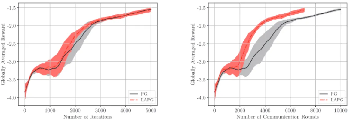
blue circles represent the agents, the stars represent the landmarks, the green arrows represent the agent-cloud communication links, and the gray arrows direct the target landmark each agent aims to cover. . . 52 3.3 Iteration and communication complexity in a heterogeneous environment (Non

momentum). The shaded region in all the figures represents the globally averaged reward distribution of each scheme within the half standard deviation of the mean. 53 3.4 Iteration and communication complexity in a heterogeneous setting (Momentum). 53 3.5 Iteration and communication complexity in a homogeneous setting (Momentum). 54 3.6 Iteration and communication complexity in a five-agent setting (RELU activation). 54 3.7 Iteration and communication complexity in a five-agent setting (Softplus). . . 55

(13)

4.1 A diagram of online geographical load balancing. Per timet, mapping nodej

has an exogenous workloadcj_t plus that stored in the queueqj_t, and schedules workloadxjk_t to data centerk. Data centerkserves an amount of workloadxk0 t

out of all the assignedxjk_t as well as that stored in the queueqk

t. The thickness of

each edge is proportional to its capacity. . . 72

4.2 Comparison of time-averaged network costs. . . 87

4.3 Instantaneous queue lengths summed over all nodes. . . 87

4.4 The evolution of stochastic multipliers at mapping node 1 (µ= 0.2). . . 88

4.5 Comparison of steady-state network costs (after106_{slots). . . .} ₈₈

4.6 Steady-state queue lengths summed over all nodes (after106_{slots). . . .} ₈₉

5.1 A diagram of online network resource allocation. Per timet, mapping node j has an exogenous workloadbj_t plus that stored in the queueq_tj, and schedules workloadxjk_t to data centerk. Data centerkserves an amount of workloadyk t out of the assignedPJ_j=1xjk_t as well as that stored in its queueq_tJ+k. The thickness of each edge is proportional to its capacity. . . 118

5.2 Time-average cost for Case 1. . . 124

5.3 Dynamic regret for Case 1. . . 125

5.4 Dynamic fit for Case 1. . . 125

5.5 Time-average cost for Case 2. . . 126

5.6 Dynamic regret for Case 2. . . 126

5.7 Dynamic fit for Case 2. . . 127

6.1 A diagram of hierarchical fog computing framework. . . 139

6.2 A comparison of OCO with full/partial-bandit feedback. . . 142

6.3 Effect of sampling schemes and number of feedback on dynamic fit. Solid lines: BanSaP with uniformly sampling from a unit sphere (uniform sampling). Dashed lines: BanSaP with randomly sampling from standard basis (coordinate sampling). 153 6.4 Effect of sampling schemes and number of feedback on average cost. Solid lines: BanSaP with sampling from a unit sphere (uniform sampling). Dashed lines: BanSaP with randomly sampling from standard basis (coordinate sampling). . . . 154

6.5 Comparison based on dynamic fit. . . 155

6.6 Comparison of average costs. The shaded region represents the cost distribution of each scheme within one standard deviation of the mean. . . 155

6.7 Impact of network size on dynamic fit per fog node. . . 156

6.8 Impact of network size on average network cost. . . 156

(14)

Chapter 1

Introduction

1.1 Motivation and context

The past decade has witnessed a proliferation of connected devices and objects, where the no-tion of Internet-of-Things (IoT) plays a central role in the envisioned technological advances. Conceptually speaking, IoT foresees an intelligent network infrastructure with ubiquitous smart devices - home automation, interactive healthcare, and self-driving connected vehicles, are typical in IoT [7, 177]. Today, a number of IoT applications have already brought major benefits to many aspects of our daily life. The current generation of IoT can already afford an increasing amount of real-time automation, and thus intelligence toward the vision of real-time IoT. However, despite the popularity of IoT, several critical challenges must be addressed before embracing its full potential [151, 4]. To this end, we highlight three key challenges that are arguably expected to be at the epicenter of emerging IoT research fields.

Extreme heterogeneity. The computational and communication capacities of connected devices differ due to differences in hardware (e.g., CPU frequency), communication protocol (e.g., ZigBee, WiFi), and energy availability (e.g., battery level) [176]. The tasks carried out on various devices are often considerably diverse, e.g., motion sensors monitor human behavior in a smart home [102], while cameras are responsible for recognizing a suspicious behavior in a crowded environment, or, vehicle plates in a parking garage.

Unpredictable dynamics. Unlike many existing communication, computing and networking platforms, the IoT dynamics can stem from multiple sources, whereadaptivityis not only critical but also essential in designing hardware and management protocols. Such sources entail human-in-the-loop dynamics in addition to physical objects [102], demand response in energy systems [56],

(15)

2 and intelligent automotive operations [101]. In these applications, IoT dynamics are intertwined with or even partially determined by human behavior [113, 121, 47] - as such, high degree of adaptivity in the algorithm and hardware design is needed.

Scalability at the core. IoT entails an intelligent network infrastructure with a massive number of devices. It is estimated that by 2020, there will be more than 50 billion devices connected through the Internet [54], which highlightsscalabilityas a key challenge for IoT [151, 7]. Scalability is not only about computational efficiency, but also about lower communication overhead (e.g., how often a device needs to communicate with the remote cloud center), as well as reduced information needed (e.g., what type of information a device needs before making sensible decisions).

Faced with these major IoT challenges, innovations in theoretical foundations and algorithmic designs for machine learning and resource management tasks in IoT are desired to enable efficient large-scale operations, and seamless co-existence of humans with things [38]. Consequently, it is imperative to develop new tools for learning and management that tap into diverse inference, signal processing, communications, and networking techniques, by drawing from fields such as machine learning, and optimization. The novel expertise gleaned from these research areas, coupled with solid analytical approaches, are the best credentials for succeeding in IoT research [151].

From a network architecture perspective, to ensure the desired user experience and meet heterogeneous service requirements, IoT tasks nowadays are no longer solely supported by the cloud data centers, but also through a promising new architecture termededge computing. This architecture distributes computation, communication, and storage closer to the end IoT devices and users, along the cloud-to-things continuum [38, 9, 10, 105, 167, 103]. In this way, delay-sensitive applications launched by a mobile device can be offloaded to the nearest mobile edge host, and the most popular contents can also be cached to minimize downloading time [40, 39].

From the algorithmic design perspective, a large volume of data is being generated from diverse IoT systems such as transportation, electric power, and computer networks, as well as the future urban infrastructure with ubiquitous smart devices. At the same time, the proliferation of optimization and machine learning advances motivates a systematic and efficient way to uncover “hidden insights” through learning from historical relationships and trends in massive datasets [164]. Learning from dynamic and large volumes of IoT data is expected to bring major science and engineering advances along with consequent improvements in quality of human life [110, 30].

(16)

1.2 Research overview

In this context, this dissertation is at the intersection of IoT, optimization, machine learning, and networking. The research presented in this dissertation focuses on building fundamental connections between methodologies from the optimization, machine learning and networking communities, and developing inter-disciplinary approaches for IoT.

It contributes answers to the following two intertwined questions.

(Q1)How can we scale up machine learning approaches for efficient IoT implementation? (Q2)How learning advances can be leveraged to enhance resource management for IoT?

The overarching objective is to wed state-of-the-art optimization and machine learning tools with the emerging IoT paradigm, in a way that they can inspire and reinforce the development of each other, with the ultimate goal of benefiting our daily life.

1.2.1 Scale up machine learning approaches for IoT

It is estimated that by 2020, there will be more than 50 billion devices connected through the Internet. To tackle(Q1), it is evident thatscalabilityandheterogeneityare two key challenges for IoT [30]. Scalability is not only about computational efficiency, but also about communication overhead of running learning algorithms at the network edge; while heterogeneity comes from both the wide range of hardware devices, as well as the diversity of tasks offered by each device. The first part of the dissertation, consisting of Chapters 2 and 3, will primarily tackle these issues. • Federated learning at the network edge. Conventional machine learning approaches require centralizing the users’ data on one machine or in a data center. Considering the massive amount of IoT devices, centralized learning becomes computationally intractable, and rises serious privacy concerns. To date, the widespread consensus is that besides data centers at the cloud, future machine learning tasks have to be performed starting from the network edge, namely mobile devices. This is the overarching goal ofedge computing, also known asfederated learning[109]. Towards this goal, this research is centered on reducing the communication overhead during the federated learning processes [31], and enhancing the robustness of learning under adversarial attacks [89]. Our learning method with adaptive communication mechanism [31] has been selected as the spotlight presentation in NeurIPS, which establishes a provably reduced communication complexity in federated learning. This part of research will be presented inChapter 2. Challenges of distributed learning also lie in asynchrony and delay introduced by e.g., IoT mobility and heterogeneity. In this context, we have developed algorithms for delayed online learning that can

(17)

4 be run asynchronously on edge devices; see our recent paper [87].

• Federated reinforcement learning over networked agents. From learning to control, reinforcement learning (RL) will play a critical role in many complex IoT tasks. Popular RL algorithms are originally developed for the single-agent tasks, but a number of IoT tasks such as autonomous vehicles and coordination of unmanned aerial vehicles (UAV), involve multiple agents operating in a distributed fashion. Today, a group of coordinated UAVs can perform traffic control, food delivery, rescue and search tasks. To coordinate agents distributed over a network however, information exchange is necessary, which requires frequent communication among agents. For resource-limited devices (e.g., battery-powered UAVs), communication is costly and the latency caused by frequent communication becomes the bottleneck of the overall performance. In this context, we have studied the distributed RL (DRL) problem that covers multi-agent collaborative RL and parallel RL. Generalizing theory and algorithms for supervised learning, an exciting communication-efficient algorithm (LAPG) is developed for DRL [29], which builds on the policy gradient (PG) method. Remarkably, the new DRL method can achieve the same order of convergence rates as plain-vanilla policy gradient under standard conditions; and, ii) reduce the communication rounds required to achieve a targeted learning accuracy, when the distributed agents are heterogeneous. Results in this line of research have been presented as part of a tutorial we delivered at MILCOM 2018, which will be presented inChapter 3.

• Scalable function approximation with unknown dynamics. Function approximation emerges at the core of machine learning tasks such as regression, classification, dimensionality re-duction, as well as reinforcement learning. Kernel methods exhibit well-documented performance in function approximation. However, the major challenges of implementing existing methods to IoT come from two sources: i) the “curse” of dimensionality in kernel-based learning; and, ii) the need to track time-varying functions with unknown dynamics. In this context, a scalable multi-kernel learning scheme has been developed to obtain the sought nonlinear learning function ‘on the fly.’ To further boost performance in unknown environments, an adaptive learning scheme has been introduced, which accounts for the unknown dynamics. So far, results in this direction have appeared in [146] and [147].

1.2.2 Rethink resource management for IoT via learning

Optimally allocating limited computing and communication resources is a crucial task in IoT. The focus of the second part in this dissertation, namely Chapters 4-6, is to tackle(Q2)by providing affirmative answers to the following intermediate questions:

(18)

(Q2a)can we learn from historical data to improve the existing resource management schemes; (Q2b)can we develop resource management schemes when the underlying models are not known?

The key novelty here is innovative statistical and interactive learning tailored for resource management tasks in IoT.

•Statistical learning viewpoint of resource management.To date, most resource manage-ment schemes for IoT are based on a pureoptimizationviewpoint (e.g., the dual (sub)gradient method), which incur large queueing delays and slow convergence. From the vantage point of IoT, the fresh idea here is to leverage the abundant historical data collected by devices, and formulate the resource management problem as an empirical risk minimization (ERM) — a central topic of statistical machine learning research [164]. In this context, we have developed a fast convergent algorithm. By cross-fertilizing advances of learning theory, we have also established the sample complexity of learning a near-optimal resource management policy [26]. To boost performance in dynamic settings, we further introduced a learn-and-adapt resource management framework [32] that will be presented inChapter 4, which capitalizes on the following features: (f1) it learns from historical data using advanced statistical learning tools; and, (f2) it efficiently adapts to IoT dynamics, and thus enables operational flexibility. Our proposed algorithms have been published in top signal processing and network optimization journals [32, 26], where we have analytically shown that this novel algorithmic design can provably improve the emerging performance tradeoff by an order of magnitude. To demonstrate the impact of this work, we have applied it to mobile computing and smart grid tasks [36, 88].

•Model-free resource management for edge computing. Typically, solving resource allo-cation problems necessitates knowledge of the models that map a resource alloallo-cation decision to its cost or utility; e.g., the model that maps transmit-power to the bit rate in communication systems. However, such models may not be available in IoT, because i) the utility function capturing e.g., service latency or reliability in edge computing, can be hard to model; and, ii) even if modeling is possible, IoT devices with limited resources may not afford the complexity of running sophisticated inference algorithms. Hence, another important aspects investigated in this part of the thesis is the feedback limited nature of resource allocation tasks in IoT. To account for physical constraints, we have considerably generalized the interactive learning tools for unconstrained problems to solve challenging constrained resource allocation problems [25]. Tailored for edge computing scenarios, we further developed a model-free online learning scheme [25] that will be presented inChapter 5, along with its bandit version [34] that will be presented inChapter 6. These algorithms come with provable performance guarantees, even when knowledge about the underlying system models

(19)

6 can be obtained only through repeated interactions with the environment.

The dissertation is summarized, and interesting open problems are included in Chapter 7.

1.3 Notational conventions

The following notation will be used throughout the subsequent chapters. Lower- (upper-) case boldface letters denote vectors (matrices). Calligraphic letters are reserved for sets, e.g.,S. Symbol >stands for matrix/vector transposition. For vectors,_k·k2ork·krepresents the Euclidean norm,

whilek·k0denotes the`0pseudo-norm counting the number of nonzero entries. The floor (ceiling)

operation _bc_c(_dc_e) denotes the largest integer no greater (the smallest integer but no smaller) than the given numberc >0;|S|counts the number of entries inS. LetN(µ,Σ)be the vector Gaussian distribution with meanµand covariance matrixΣ.

(20)

Chapter 2

Federated learning at the network edge

2.1 Introduction

In this paper, we develop communication-efficient algorithms to solve the following problem

min

θ∈Rd L

(θ) with _L(θ) := X

m∈M

Lm(θ) (2.1)

whereθ∈Rdis the unknown vector,Land{Lm, m∈M}are smooth (but not necessarily convex)

functions with_M:=_{1, . . . , M_}. Problem (2.1) naturally arises in a number of areas, such as multi-agent optimization [115], distributed signal processing [57, 136], and distributed machine learning [44]. Considering the distributed machine learning paradigm, eachLm is also a sum of

functions, e.g.,Lm(θ) :=Pn∈Nm`n(θ), where`nis the loss function (e.g., square or the logistic

loss) with respect to the vectorθ(describing the model) evaluated at the training samplexn; that is,

`n(θ) :=`(θ;xn). While machine learning tasks are traditionally carried out at a single server, for

datasets with massive samples{xn}, running gradient-based iterative algorithms at a single server can be prohibitively slow; e.g., the server needs to sequentially compute gradient components given limited processors. A simple yet popular solution in recent years is to parallelize the training across multiple computing units (a.k.a. workers) [44]. Specifically, assuming batch samples distributedly stored in a total ofM workers with the workerm _{∈ M}associated with samples {xn, n∈ Nm}, a globally shared modelθwill be updated at the central server by aggregating

gradients computed by workers. Due to bandwidth and privacy concerns, each workermwill not upload its data{xn, n∈ Nm}to the server, thus the learning task needs to be performed by

iteratively communicating with the server.

(21)

8 We are particularly interested in the scenarios where communication between the central server and the local workers is costly, as is the case with the Federated Learning paradigm [109, 150], and the cloud-edge AI systems [153]. In those cases, communication latency is the bottleneck of overall performance. More precisely, the communication latency is a result of initiating communication links, queueing and propagating the message. For sending small messages, e.g., thed-dimensional modelθor aggregated gradient, this latency dominates the message size-dependent transmission latency. Therefore, it is important to reduce the number of communication rounds, even more so than the bits per round. In short, our goal is to find θ that minimizes (2.1) using as low communication overhead as possible.

2.1.1 Prior art

To put our work in context, we review prior contributions that we group in two categories.

Large-scale machine learning. Solving (2.1) at a single server has been extensively studied for large-scale learning tasks, where the “workhorse approach” is the simple yet efficient stochastic gradient descent (SGD) [131, 18, 19]. For learning beyond a single server, distributed parallel machine learning is an attractive solution to tackle large-scale learning tasks, where the parameter server architecture is the most commonly used one [44, 91]. Different from the single server case, parallel implementation of the batch gradient descent (GD) is a popular choice, since SGD that has low complexity per iteration requires a large number of iterations thus communication rounds [110]. For traditional parallel learning algorithms however, latency, bandwidth limits, and unexpected drain on resources, that delay the update of even a single worker will slow down the entire system operation. Recent research efforts in this line have been centered on understanding asynchronous-parallel algorithms to speed up machine learning by eliminating costly synchronization; e.g., [23, 156, 126, 129, 96].

Communication-efficient learning. Going beyond single-server learning, the high communica-tion overhead becomes the bottleneck of the overall system performance [110]. Communicacommunica-tion- Communication-efficient learning algorithms have gained popularity [73, 182]. Distributed learning approaches have been developed based on quantized (gradient) information, e.g., [157], but they only reduce the required bandwidth per communication, not the rounds. For machine learning tasks where the loss function is convex and its conjugate dual is expressible, the dual coordinate ascent-based approaches have been demonstrated to yield impressive empirical performance [150, 72, 104]. But these algorithms run in a double-loop manner, and the communication reduction has not

(22)

been formally quantified. To reduce communication by accelerating convergence, approaches leveraging (inexact) second-order information have been studied in [144, 183]. Roughly speaking, algorithms in [150, 72, 104, 144, 183] reduce communication by increasing local computation (relative to GD), while our method does not increase local computation. In settingsdifferentfrom the one considered in this paper, communication-efficient approaches have been recently studied with triggered communication protocols [98, 83]. Except for convergence guarantees however, no theoretical justification for communication reduction has been established in [98]. While a sublinear convergence rate can be achieved by algorithms in [83], the proposed gradient selection rule is nonadaptive and requires double-loop iterations.

2.1.2 Our contributions

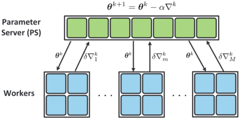
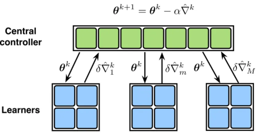
Before introducing our approach, we revisit the popular GD method for (2.1) in the setting of one parameter server andM workers: At iterationk, the server broadcasts the current modelθk_to_all

the workers; every workerm ∈ Mcomputes∇Lm θk

and uploads it to the server; and once receiving gradients from all workers, the server updates the model parameters via

GD iteration θk+1=θk₋α_∇k_GD with _∇k_GD:= X m∈M

∇Lm θk

(2.2)

whereαis a stepsize, and_∇k_GDis an aggregated gradient that summarizes the model change. To implement (2.2), the server has to communicate withallworkers to obtain fresh{∇Lm θk

}. In this context, the present paper puts forward a new batch gradient method (as simple as GD) that canskipcommunication at certain rounds, which justifies the termLazilyAggregated

Gradient (LAG). With its derivations deferred to Section 2.2, LAG resembles (2.2), given by

LAG iteration θk+1=θk−α∇k _with _∇k_:= X m∈M

∇Lm θˆkm

(2.3)

where each∇Lm(ˆθk_m)is either∇Lm(θk), whenˆθk_m =θk, or an outdated gradient that has been computed using an old copyθˆk_m ₆=θk. Instead of requesting fresh gradient from every worker in (2.2), the twist is to obtain∇k_{by refining the previous aggregated gradient}_∇k−1_{; that is, using}

only the new gradients from theselectedworkers inMk_{, while reusing the outdated gradients}

from the rest of workers. Therefore, withθˆk

(23)

10

Parameter Server (PS)

Workers

Figure 2.1: LAG for distributed machine learning in a parameter server setup.

(2.3) is equivalent to

LAG iteration θk+1=θk−α∇k _with _∇k₌_∇k−1

+X

m∈Mk

δ∇k

m (2.4)

whereδ_∇k

m :=∇Lm(θk)−∇Lm(ˆθk−1m )is the difference between two evaluations of∇Lmat the

current iterateθkand the old copyθˆk−1_m . If∇k−1_{is stored in the server, this simple modification}

scales down the number of communication rounds from GD’sMto LAG’s_|Mk_|.

We develop two different rules to selectMk_{. The first rule is adopted by the parameter server}

(PS), and the second one by every worker (WK). At iterationk,

LAG-PS: the server determinesMk_{and sends}_θk_{to the workers in}_Mk_{; each worker}_m_∈Mk

computes_∇Lm(θk)and uploadsδ_∇k

m; workers inMkdo nothing; the server updates via (2.4);

LAG-WK: the server broadcastsθkto all workers; every worker computes∇Lm(θk), and checks if it belongs to_Mk; only the workers in_Mkuploadδ_∇k

m; the server updates via (2.4).

See a comparison of two LAG variants with GD in Table 2.1.

Naively reusing outdated gradients, while saving communication per iteration, can increase the total number of iterations. To keep this number in control, we judiciously design our simple trigger rules so that LAG can: i) achieve the same order of convergence rates (thus iteration complexities) as batch GD under strongly-convex, convex, and nonconvex smooth cases; and, ii) requirereducedcommunication to achieve a targeted learning accuracy, when the distributed datasets are heterogeneous (measured by certain quantity specified later). In certain learning settings, LAG requires onlyO(1/M)communication of GD. Empirically, we found that LAG can reduce the communication required by GD and other distributed parallel learning methods by

(24)

Metric Communication Computation Memory Algorithm PS_→WKm WKm_→PS PS WKm PS WKm GD θk ∇Lm (2.2) ∇Lm θk / LAG-PS θk, ifm_∈Mk_δ ∇k m, ifm∈Mk (2.4), (2.15b)∇Lm, ifm∈Mk θk,∇k,{θˆkm} ∇Lm(ˆθkm) LAG-WK θk δ_∇k m, ifm∈Mk (2.4) ∇Lm,(2.15a) θk,∇k ∇Lm(ˆθkm)

Table 2.1: A comparison of communication, computation and memory requirements.PSdenotes the parameter server,WKdenotes the worker,PS_→WKmis the communication link from the server to workerm, andWKm→PSis the communication link from workermto the server. several orders of magnitude.

Notation. Bold lowercase letters denote column vectors, which are transposed by(_·)>_{. And}_k_x_k

denotes the`2-norm ofx. Inequalities for vectorsx>0is defined entrywise.

2.2 LAG: Lazily aggregated gradient approach

In this section, we formally develop our LAG method, and present the intuition and basic principles behind its design. The original idea of LAG comes from a simple rewriting of the GD iteration (2.2) as θk+1 ₌_θk₋_α X m∈M ∇Lm(θk−1)−α X m∈M ∇Lm θk − ∇Lm θk−1 . (2.5)

Let us view∇Lm(θk)−∇Lm(θk−1)as a refinement to∇Lm(θk−1), and recall that obtaining this refinement requires a round of communication between the server and the workerm. There-fore, to save communication, we can skip the server’s communication with the worker m if this refinement is small compared to the old gradient; that is, k∇Lm(θk)− ∇Lm(θk−1)k kP

m∈M∇Lm(θk−1)k.

Generalizing on this intuition, given the generic outdated gradient components{∇Lm(ˆθk−1_m )}

withθˆk−_m1=θk−1−τmk−1

m for a certainτmk−1≥0, if communicating with some workers will bring only

small gradient refinements, we skip those communications (contained in setMk

c) and end up with

θk+1 ₌_θk₋_α X m∈M ∇Lm θˆk−1m −α X m∈Mk ∇Lm θk − ∇Lm ˆθk−1m (2.6a) =θk−α∇L(θk)−α X m∈Mk c ∇Lm ˆθk−1m − ∇Lm θk (2.6b)

(25)

12 whereMk _and _Mk

c are the sets of workers that doanddo not communicate with the server,

respectively. It is easy to verify that (2.6) is identical to (2.3) and (2.4). Comparing (2.2) with (2.6b), whenMk

c includes more workers, more communication is saved, butθkis updated by a

coarser gradient.

Key to addressing this communication vs accuracy tradeoff is a principled criterion to select a subset of workers_Mk_c that do not communicate with the server at each round. To achieve this “sweet spot,” we will rely on the fundamental descent lemma. For GD, it is given as follows [119].

Lemma 1 (GD descent in objective). Suppose _L(θ) is L-smooth, and ¯θk+1 is generated by running one-step GD iteration(2.2)givenθk_{and stepsize}_α_{. Then the objective values satisfy}

L(¯θk+1)_{− L}(θk)_{≤ −} α₋α 2_L 2 k∇L(θk)_k2 := ∆k_GD(θk). (2.7) Likewise, for our wanted iteration (2.6), the following holds; its proof is given in the Supple-ment.

Lemma 2 (LAG descent in objective). Suppose_L(θ) isL-smooth, and θk+1 is generated by running one-step LAG iteration(2.4)givenθk_{. The objective values satisfy (cf.}_δ_∇k

min(2.4)) L(θk+1)−L(θk)≤−α₂ ∇L₍_θk₎ 2 +α 2 X m∈Mk c δ∇k m 2 + L 2− 1 2α θ k+1 −θk 2 := ∆kLAG(θ k ). (2.8)

Lemmas 1 and 2 estimate the objective value descent by performing one-iteration of the GD and LAG methods, respectively, conditioned on a common iterate θk_{. GD finds}_∆k

GD(θ

k

)by performingM rounds of communication with all the workers, while LAG yields∆k

LAG(θk)by

performing only|Mk_|_{rounds of communication with a selected subset of workers. Our pursuit is}

to selectMk_{to ensure that}_{LAG enjoys larger per-communication descent than GD}_{; that is}

∆k LAG(θ k₎ |Mk_| ≤ ∆k GD(θ k₎ M . (2.9)

If we choose the standardα= 1/Lin Lemmas 1 and 2, it follows that

∆k GD(θk) :=− 1 2L ∇L(θ k₎ 2 ∆k_LAG(θk) :=₋ 1 2L ∇L(θ k₎ 2 + 1 2L X m∈Mk c ∇Lm θˆk−1m − ∇Lm θk 2 . (2.10a) (2.10b)

(26)

Plugging (2.10) into (2.9), and rearranging terms, (2.9) is equivalent to X m∈Mk c ∇Lm θˆk−1m −∇Lm θk 2 ≤ M k c ∇L(θ k₎ 2. M. (2.11)

Note that since we have

X m∈Mk c ∇Lm θˆk−1m −∇Lm θk 2 ≤ M k c X m∈Mk c ∇Lm ˆ θk−1_m −∇Lm θk 2 (2.12)

if we can further show that

∇Lm ˆ θk−1_m −∇Lm θk 2 ≤ ∇L(θ k₎ 2. M2_, _∀_m_{∈ M}k c. (2.13)

then we can prove that (2.11) holds thus (2.9) also holds.

However, directly checking (2.13) at each worker is expensive since i) obtainingk∇L(θk)k2

requires information from all the workers; and ii) each worker does not know_Mk_c. Instead, we approximatek∇L(θk₎_k2_{in (2.13) by} ∇L(θ k₎ 2 ≈ 1 α2 D X d=1 ξd θ k+1−d −θk−d 2 (2.14)

where_{ξd}Dd=1are constant weights. The rationale here is that, asLis smooth,∇L(θk)cannot be

very different from the recent gradients or the recent iteratelags.

Building upon (2.13) and (2.14), we will include workermin_Mk_c of (2.6) if it satisfies

LAG-WK condition ∇Lm(ˆθ k−1 m )−∇Lm(θk) 2 ≤_α₂1_M₂ D X d=1 ξd θ k+1−d −θk−d 2 . (2.15a)

Condition (2.15a) is checked atthe worker sideafter each worker receivesθkfrom the server and computes its_∇Lm(θk). If broadcasting is also costly, we can resort to the followingserver side

rule: LAG-PS condition L2_m ˆ θk−1_m −θk 2 ≤ 1 α2_M2 D X d=1 ξd θ k+1−d −θk−d 2 . (2.15b)

(27)

14

Algorithm 1LAG-WK

1: Input:Stepsizeα >0, and_{ξd}.

2: Initialize:θ1,_{∇Lm(ˆθ0m),∀m}.

3: fork= 1,2, . . . , Kdo

4: Serverbroadcastsθkto all workers.

5: forworkerm= 1, . . . , Mdo 6: Workermcomputes_∇Lm(θk).

7: Workermcheckscondition (2.15a).

8: ifworkermviolates (2.15a)then 9: Workermuploadsδ∇k

m.

10: .Save_∇Lm(ˆθkm) =∇Lm(θk)

11: else

12: Workermuploads nothing.

13: end if

14: end for

15: Serverupdatesvia (2.4).

16: end for

Algorithm 2LAG-PS

1: Input:Stepsizeα >0,_{ξd}, andLm,∀m.

2: Initialize:θ1,_{θˆ0m,∇Lm(ˆθ0m),∀m}.

3: fork= 1,2, . . . , Kdo

4: forworkerm= 1, . . . , Mdo 5: Servercheckscondition (2.15b).

6: ifworkermviolates (2.15b)then 7: Serversendsθkto workerm.

8: .Saveθˆkm=θkat server

9: Workermcomputes_∇Lm(θk).

10: Workermuploadsδ∇k m.

11: else

12: No actions at server and workerm.

13: end if

14: end for

15: Serverupdatesvia (2.4).

16: end for

Table 2.2: A comparison of LAG-WK and LAG-PS.

The values of_{ξd}andDadmit simple choices, e.g., ξd = 1/D, ∀dwithD = 10used in the

simulations.

LAG-WK vs LAG-PS. To perform (2.15a), the server needs to broadcast the current modelθk, and all the workers need to compute the gradient; while performing (2.15b), the server needs the estimated smoothness constantLm for all the local functions. On the other hand, as it will be

shown in Section 2.3, (2.15a) and (2.15b) lead to the same worst-case convergence guarantees. In practice, however, the server-side condition is more conservative than the worker-side one at communication reduction, because the smoothness of_Lmreadily implies that satisfying (2.15b)

will necessarily satisfy (2.15a), but not vice versa. Empirically, (2.15a) will lead to a largerMk c

than that of (2.15b), and thus extra communication overhead will be saved. Hence, (2.15a) and (2.15b) can be chosen according to users’ preferences. LAG-WK and LAG-PS are summarized as Algorithms 1 and 2.

Regarding our proposed LAG method, two remarks are in order.

R1) With recursive update of the lagged gradients in (2.4) and the lagged iterates in (2.15), implementing LAG is as simple as GD; see Table 2.1. Both empirically and theoretically, we will further demonstrate that using lagged gradients even reduces the overall delay by cutting down costly communication.

(28)

gradient, Nesterov’s acceleration, dual coordinate ascent and second-order methods, LAG is not orthogonal to all of them. Instead, LAG can be combined with these methods to develop even more powerful learning schemes. Extension to the proximal LAG is also possible to cover nonsmooth regularizers.

2.3 Iteration and communication complexity

In this section, we establish the convergence of LAG, under the following standard conditions.

Assumption 1: Loss function_Lm(θ)isLm-smooth, andL(θ)isL-smooth.

Assumption 2:L(θ)is convex and coercive.

Assumption 3: _L(θ) isµ-strongly convex, or generally, satisfies the Polyak-Łojasiewicz (PL) condition with the constantµ; that is,2µ(L(θk)− L(θ∗))≤ k∇L(θk)k2_.

Note that the PL condition in Assumption 3 is strictly weaker than the strongly convexity (or even convexity), and it is satisfied by a wider range of machine learning problems such as least squares for underdetermined linear systems and logistic regression; see details in [77]. While the PL condition is sufficient for the subsequent linear convergence analysis, we will still use the strong convexity for the ease of understanding by a wide audience.

The subsequent analysis critically builds on the followingLyapunov function:

Vk:=_L(θk)_{− L}(θ∗) + D X d=1 βd θ k+1−d −θk−d 2 (2.16)

whereθ∗is the minimizer of (2.1), and_{βd}are constants that will be determined later.

We will start with the sufficient descent of ourVkin (2.16).

Lemma 3(descent lemma). Under Assumption 1, ifαand_{ξd}are chosen properly, there exist

constantsc0,· · ·, cD ≥0such that the Lyapunov function in(2.16)satisfies

Vk+1₋Vk_{≤ −}c0 ∇L(θ k₎ 2 − D X d=1 cd θ k+1−d −θk−d 2 (2.17)

which implies the descent in our Lyapunov function, that is,Vk+1_≤Vk.

Lemma 3 is a generalization of GD’s descent lemma. As specified in the supplementary material, under properly chosen_{ξd}, the stepsizeα∈(0,2/L)includingα = 1/Lguarantees

(29)

16 (2.17), matching the stepsize region of GD. WithMk ₌_M_and_β

d= 0,∀din (2.16), Lemma 3

reduces to Lemma 1.

2.3.1 Convergence in strongly convex case

We first present the convergence under the smooth and strongly convex condition.

Theorem 1(strongly convex case). Under Assumptions 1 and 3, the iterates_{θk}generated by LAG-WK or LAG-PS satisfy

L θK

− L θ∗

≤ 1₋c(α;_{ξd}) K

V0 (2.18)

whereθ∗is the minimizer of_L(θ)in(2.1), andc(α;{ξd}) ∈(0,1)is a constant depending on

α, _{ξd}and{βd}as well as the condition numberκ:=L/µthat are specified in the

supplemen-tary material.

Iteration complexity. The iteration complexity in its generic form is complicated sincec(α;{ξd})

depends on the choice of several parameters. Specifically, if we choose the parameters as follows

ξ1 =· · ·=ξD :=ξ < 1 D, α:= 1₋√Dξ L , β1 =· · ·=βD := D₋d+ 1 2αpD/ξ (2.19)

then, following Theorem 1, the iteration complexity of LAG in this case is

ILAG() =

κ

1₋√Dξ log

−1

. (2.20)

The iteration complexity in (2.20) is on the same order of GD’s iteration complexityκlog(−1), but has a worse constant. This is the consequence of using a smaller stepsize in (2.19) (relative toα= 1/Lin GD) to simplify the choice of other parameters. Empirically, LAG withα= 1/L

can achieve almost the same empirical iteration complexity as GD; see Section 2.4. Building on the iteration complexity, we study next thecommunication complexityof LAG. In the setting of our interest, we define the communication complexity as thetotal number of uploadsover all the workers needed to achieve accuracy. While the accuracy refers to the objective optimality error in the strongly convex case, it is considered as the gradient norm in general (non)convex cases.

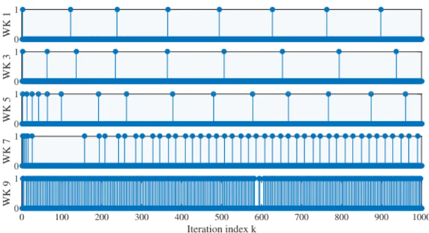
The power of LAG is best illustrated by numerical examples; see an example of LAG-WK in Figure 2.2. Clearly, workers with a small smoothness constant communicate with the server less frequently. This intuition will be formally treated in the next lemma.

(30)

0 1 WK 1 0 1 WK 3 0 1 WK 5 0 1 WK 7 0 100 200 300 400 500 600 700 800 900 1000 Iteration index k 0 1 WK 9

Figure 2.2: Communication events of workers1,3,5,7,9over1,000iterations. Each stick is an upload. An example withL1< . . . < L9.

Lemma 4(lazy communication). Define the importance factor of every workermas_H(m) :=

Lm/L. If the stepsizeαand the constants{ξd}in(2.15)satisfyξD ≤ · · · ≤ξd≤ · · · ≤ ξ1and

workermsatisfies

H2(m)_≤ξd

(dα2L2M2) :=γd (2.21)

then, until iterationk, workermcommunicates with the server at mostk/(d+ 1)rounds.

Lemma 4 asserts that if the workermhas a smallLm(a close-to-linear loss function) such that

H2₍_m₎_≤_γ

d, then under LAG, it only communicates with the server at mostk/(d+ 1)rounds.

This is in contrast to the total ofkcommunication rounds involved per worker under GD. Ideally, we want as many workers satisfying (2.21) as possible, especially whendis large.

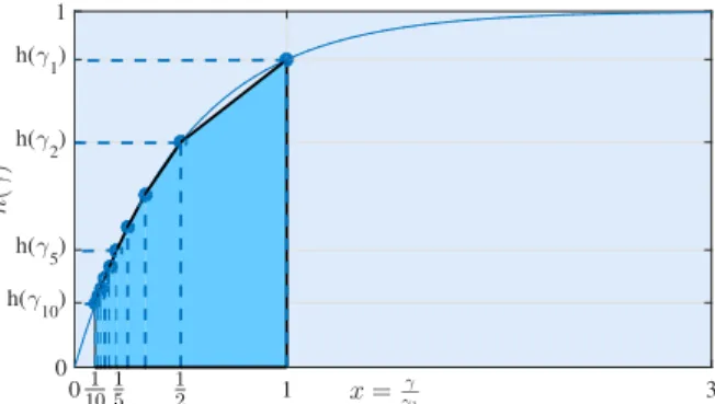
To quantify the overall communication reduction, we will rely on what we term the hetero-geneity score function, given by

h(γ) := 1

M

X

m∈M

1(H2(m)_≤γ) (2.22)

where the indicator1equals1whenH2(m)≤γholds, and0otherwise. Clearly,h(γ)is a nonde-creasing function ofγ, that depends on the distribution of smoothness constantsL1, L2, . . . , LM.

It is also instructive to view it as the cumulative distribution function of thedeterministicquantity

H2(m), implyingh(γ)_∈[0,1]. Putting it in our context, the critical quantityh(γd)lower bounds

the fraction of workers that communicate with the server at mostk/(d+ 1)rounds until thek-th iteration.

(31)

18

Proposition 1(communication complexity). Under the same conditions as those in Theorem 1, withγddefined in(2.21)and the functionh(γ)defined in(2.22), the communication complexity of

LAG denoted asCLAG()is bounded by

CLAG()_≤ 1₋ D X d=1 1 d− 1 d+ 1 h(γd) MILAG() := 1₋∆¯C(h;_{γd}) MILAG() (2.23)

where the constant is defined as∆¯C(h;{γd}) :=PD_d=1 1_d−_d+11

h(γd).

The communication complexity in (2.23) crucially depends on the iteration complexityILAG()

as well as what we call the fraction of reduced communication per iteration ∆¯C(h;_{γd}).

Simply choosing the parameters as (2.19), it follows from (2.20) and (2.23) that (cf. γd =

ξ(1₋√Dξ)−2_M−2_d−1₎

CLAG()≤ 1−∆¯C(h;ξ)

CGD()

1−pDξ

. (2.24)

where the GD’s complexity isCGD() = M κlog(−1). In (2.24), due to the nondecreasing

property ofh(γ), increasing the constantξyields a smaller fraction of workers1−∆¯C(h;ξ)that are communicating per iteration, yet with a larger number of iterations (cf. (2.20)). The key enabler of LAG’s communication reduction is a heterogeneous environment associated with a favorable

h(γ)ensuring that the benefit of increasing ξ is more significant than its effect on increasing iteration complexity. More precisely, for a givenξ, ifh(γ)guarantees∆¯C(h;ξ)>√Dξ, then we

haveCLAG()<CGD(). Intuitively speaking, if there is a large fraction of workers with small

Lm, LAG has lower communication complexity than GD. An example follows to illustrate this

reduction.

Example. ConsiderLm = 1, m 6= M, andLM = L ≥ M2 1, where we haveH(m) = 1/L, m6=M, H(M) = 1, implying thath(γ) ≥1− 1 M, ifγ ≥1/L2. ChoosingD ≥M and ξ =M2_D/L2 _<₁_/D_{in (2.19) such that}_γ D ≥1/L2in (2.21), we have (cf. (2.24)) CLAG() CGD()_≤ 1₋ 1₋ 1 D+ 1 1₋ 1 M _. 1₋M D/L_≈ M+D M(D+ 1) ≈ 2 M. (2.25) Due to technical issues in the convergence analysis, the current condition onh(γ)to ensure LAG’s communication reduction is relatively restrictive. Establishing communication reduction on a broader learning setting that matches the LAG’s intriguing empirical performance is in our research agenda.

(32)

2.3.2 Convergence in (non)convex case

LAG’s convergence and communication reduction guarantees go beyond the strongly-convex case. We next establish the convergence of LAG for general convex functions.

Theorem 2(convex case). Under Assumptions 1 and 2, ifαand_{ξd}are chosen properly, then

the iterates_{θk_}generated by LAG-WK or LAG-PS satisfy

L(θK)− L(θ∗) =O(1/K). (2.26) For nonconvex objective functions, LAG can guarantee the following convergence result.

Theorem 3(nonconvex case). Under Assumption 1, ifαand_{ξd}are chosen properly, then the

iterates_{θk_}generated by LAG-WK or LAG-PS satisfy

min 1≤k≤K θk+1−θk 2 =o(1/K) and min 1≤k≤K ∇L(θk) 2 =o(1/K). (2.27)

Theorems 2 and 3 assert that with the judiciously designed lazy gradient aggregation rules, LAG can achieve order of convergence rate identical to GD for general convex and nonconvex smooth objective functions. Furthermore, we next show that in these general cases, LAG still requires fewer communication rounds than GD, under certain conditions on the heterogeneity functionh(γ).

In the general smooth (possibly nonconvex) case however, we define the communication complexity in terms of achieving-gradient error; e.g.,mink=1,···,Kk∇L(θk)k2≤. Similar to

Proposition 1, we present the communication complexity as follows.

Proposition 2. 2[communication complexity] Under Assumption 1, with∆¯C(h;_{γd})defined as

in Proposition 1, the communication complexity of LAG denoted asCN−LAG()is bounded by

CN−LAG()≤ 1−∆¯C(h;{γd})

CN−GD()

(1₋PD_d=1ξd)

(2.28)

whereCN−GD()is the communication complexity of GD. Choosing the parameters as(2.19), if the heterogeneity functionh(γ)satisfies that there existsγ0_{such that}_γ0 _< h(γ0₎

(D+1)DM2, then we

have that

(33)

20 Along with Proposition 1, we have shown that for strongly convex, convex, and nonconvex smooth objective functions, LAG enjoys provably lower communication overhead relative to GD in certain heterogeneous learning settings. In fact, the LAG’s empirical performance gain over GD goes far beyond the above worst-case theoretical analysis, and lies in a much broader distributed learning setting, which is confirmed by the subsequent numerical tests.

2.4 Numerical tests

To validate the theoretical results, this section evaluates the empirical performance of LAG in linear and logistic regression tasks. All experiments were performed using MATLAB on an Intel CPU @ 3.4 GHz (32 GB RAM) desktop.

For linear regression task, consider the square loss function at workermas

Lm(θ) := X n∈Nm yn−x>nθ 2 (2.30)

where{xn, yn,∀n∈ Nm}are data at workerm.

Real datasets. Performance is tested on the following benchmark datasets [93]; see Table 2.3. • Housingdataset [63] contains 506samples(xn, yn) withyn representing the median value

of house price, which is affected by features in xnsuch as per capita crime rate and weighted

distances to five Boston employment centers.

•Body fatdataset contains252samples(xn, yn)withyndescribing the percentage of body fat,

which is determined by underwater weighing and various body measurements inxn.

•Abalonedataset contains417samples(xn, yn)withynfor the age of abalone andxnfor the

physical measurements of abalone, e.g., sex, height, and shell weight.

Dataset # features(d) # samples(N) worker index

Housing 13 506 1,2,3

Body fat 14 252 4,5,6

Abalone 8 417 7,8,9

Table 2.3: A summary of real datasets used in the linear regression tests.

For logistic regression, consider the binary logistic regression problem

Lm(θ) := X n∈Nm log1 + exp(−ynx>nθ) +λ 2kθk 2_. _(2.31)

(34)

Dataset # features(d) # samples(N) worker index

Ionosphere 34 351 1,2,3

Adult fat 113 1605 4,5,6

Derm 34 358 7,8,9

Table 2.4: A summary of real datasets used in the logistic regression tests.

whereλ= 10−3 is the regularization constant.

Real datasets. Performance is tested on the following datasets; see a summary in Table 2.4. •Ionospheredataset [148] is to predict whether it is a “good” radar return or not – “good” if the features inxnshow evidence of some structures in the ionosphere.

•Adultdataset [79] contains samples that predict whether a person makes over50Ka year based on features inxnsuch as work-class, education, and marital-status.

•Dermdataset [61] for differential diagnosis of erythemato-squaxous diseases, which is deter-mined by clinical and histopathological attributes inxnsuch as erythema, family history, focal hypergranulosis and melanin incontinence.

By default, we consider one server, and nine workers. Throughout the test, we use the optimality error in objective_L(θk₎_{− L}_(θ∗₎_{as figure of merit of our solution. To benchmark LAG,}

we consider the following approaches.

.Cyc-IAGis the cyclic version of the incremental aggregated gradient (IAG) method [16, 60] that resembles the recursion (2.4), but communicates with one worker per iteration cyclically.

.Num-IAGalso resembles the recursion (2.4), but it randomly selects one worker to obtain a fresh gradient per iteration with the probability of choosing workermequal toLm/Pm∈MLm.

.Batch-GDis the GD iteration (2.2) that communicates with all the workers per iteration. For LAG-WK, we chooseξd=ξ = 1/DwithD= 10, and for LAG-PS, we choose more

aggressiveξd=ξ = 10/DwithD= 10. Stepsizes for LAG-WK, LAG-PS, and GD are chosen as

α= 1/L; to optimize performance and guarantee stability, stepsizes for Cyc-IAG and Num-IAG are chosen asα = 1/(M L). For the linear regression task, no regularization is added; for the logistic regression task, the`2-regularization parameter is set toλ= 10−3.

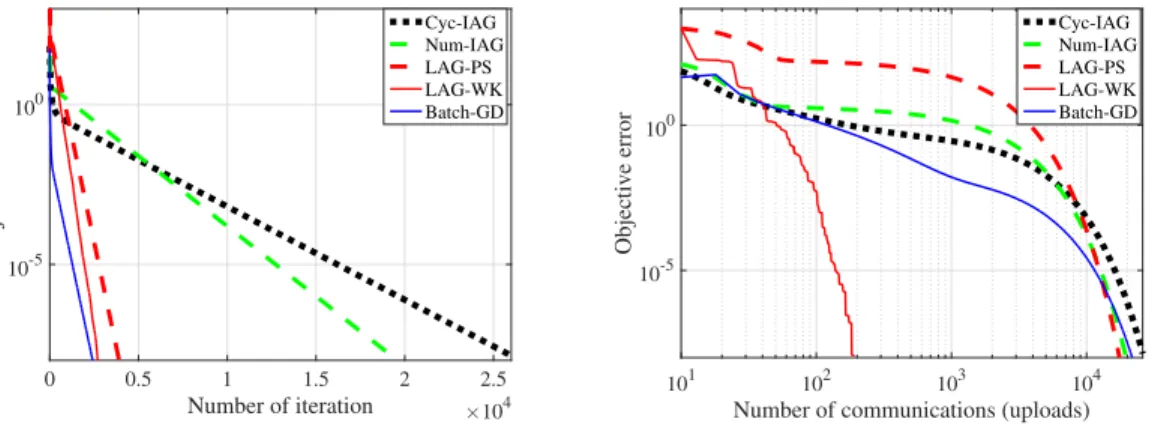
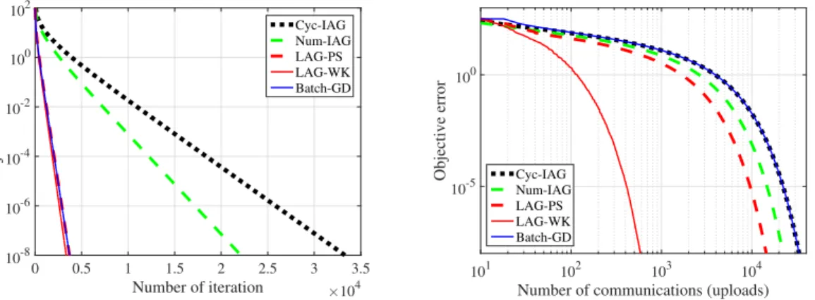
We consider twosynthetic datatests: a) linear regression with increasing smoothness con-stants, e.g., Lm = (1.3m−1 + 1)2,∀m; and, b) logistic regression with uniform smoothness

constants, e.g.,L1 =. . .= L9 = 4. For each worker, we generate 50 samplesxn ∈R50from

the standard Gaussian distribution, and rescale the data to mimic the increasing and uniform smoothness constants. For the case of increasingLm, it is not surprising that both LAG variants

(35)

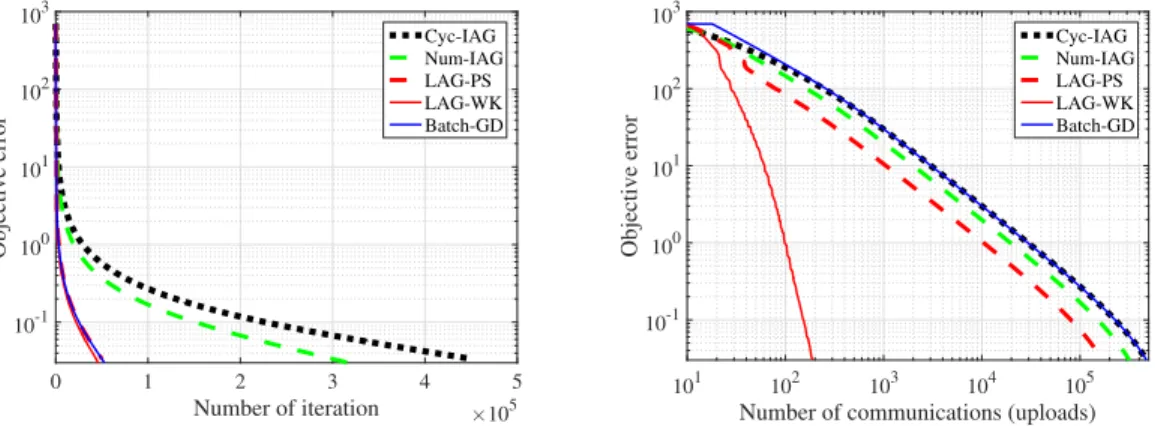
22 200 400 600 800 1000 Number of iteration 10-5 100 Objective error Cyc-IAG Num-IAG LAG-PS LAG-WK Batch-GD 101 102 103

Number of communications (uploads)

10-5

100

Objective error Cyc-IAGNum-IAG

LAG-PS LAG-WK Batch-GD

Figure 2.3: Iteration and communication complexity in synthetic datasets with increasingLm.

0 0.5 1 1.5 2 2.5 Number of iteration ×104 10-5 100 Objective error Cyc-IAG Num-IAG LAG-PS LAG-WK Batch-GD 101 102 103 104

10-5 100 Objective error Cyc-IAG Num-IAG LAG-PS LAG-WK Batch-GD

Figure 2.4: Iteration and communication complexity in synthetic datasets with uniformLm.

still has marked improvements on communication, thanks to its ability of exploiting thehidden

smoothness of the loss functions; that is, the local curvature ofLmmay not be as steep asLm; see

Figure 2.4.

Performance is also tested on thereal datasets[93]: a) linear regression usingHousing,Body fat,Abalonedatasets; and, b) logistic regression usingIonosphere,Adult,Dermdatasets; see Figures 2.5-2.6. Each dataset is evenly split into three workers with the number of features used in the test equal to the minimal number of features among all datasets. In all tests, LAG-WK outper-forms the alternatives in terms of both metrics, especially reducing the needed communication rounds by several orders of magnitude. Its needed communication rounds can be evensmallerthan the number of iterations, if none of workers violate the trigger condition (2.15) at certain iterations. Additional tests on real datasets under different number of workers are listed in Table 2.5. Under all the tested settings, LAG-WK consistently achieves the lowest communication complexity,

(36)

0 1000 2000 3000 4000 5000 Number of iteration 10-5 100 105 Objective error Cyc-IAG Num-IAG LAG-PS LAG-WK Batch-GD 101 102 103 104

10-5 100 105 Objective error Cyc-IAG Num-IAG LAG-PS LAG-WK Batch-GD

Figure 2.5: Iteration and communication complexity for linear regression in real datasets.

0 0.5 1 1.5 2 2.5 3 3.5 Number of iteration _×104 10-8 10-6 10-4 10-2 100 102 Objective error Cyc-IAG Num-IAG LAG-PS LAG-WK Batch-GD 101 102 103 104

10-5 100

Objective error Cyc-IAG Num-IAG LAG-PS LAG-WK Batch-GD

Figure 2.6: Iteration and communication complexity for logistic regression in real datasets.

which corroborates the effectiveness of LAG when it comes to communication reduction. Similar performance gain has also been observed in the test on a larger datasetGisette. The Gisette dataset was constructed from the MNIST data [85]. After random selecting subset of samples and eliminating all-zero features, it contains2000samplesxn∈R4837. We randomly split this dataset into nine workers. The performance of all the algorithms is reported in Figure 2.7 in terms of the iteration and communication complexity. Clearly, LAG-WK and LAG-PS achieve the same iteration complexity as GD, and outperform Cyc- and Num-IAG. Regarding communication complexity, two LAG variants reduce the needed communication rounds by several orders of magnitude compared with the alternatives.

(37)

24

Linear regression Logistic regression

Algorithm M = 9 M = 18 M = 27 M = 9 M = 18 M = 27 Cyclic-IAG 5271 10522 15773 33300 65287 97773 Num-IAG 3466 5283 5815 22113 30540 37262 LAG-PS 1756 3610 5944 14423 29968 44598 LAG-WK 412 657 1058 584 1098 1723 Batch GD 5283 10548 15822 33309 65322 97821

Table 2.5: Communication complexity (= 10−8) under different number of workers.

0 1 2 3 4 5 Number of iteration _×₁₀5 10-1 100 101 102 103 Objective error Cyc-IAG Num-IAG LAG-PS LAG-WK Batch-GD 101 102 103 104 105

10-1 100 101 102 103 Objective error Cyc-IAG Num-IAG LAG-PS LAG-WK Batch-GD

Figure 2.7: Iteration and communication complexity in Gisette dataset.

2.5 Proofs of lemmas and theorems

2.5.1 Proof of Lemma 2

Using the smoothness ofL(_·)in Assumption 1, we have that L(θk+1)_{− L}(θk)_≤D_∇L(θk),θk+1₋θkE+L 2 θ k+1 −θk 2 . (2.32) Plugging (2.6) into_∇L(θk),θk+1₋θk leads to (cf.θˆk_m = ˆθk−1_m ,_∀m_{∈ M}k c) D ∇L(θk),θk+1−θkE =₋α * ∇L(θk),_∇L(θk) + X m∈Mk c ∇Lm θˆkm − ∇Lm θk + =−α ∇L(θ k₎ 2 −α * ∇L(θk), X m∈Mk c ∇Lm ˆθkm − ∇Lm θk +

(38)

=₋α ∇L(θ k₎ 2 + * −√α_∇L(θk),√α X m∈Mk c ∇Lm θˆkm − ∇Lm θk + . (2.33)

Using2a>_b₌_k_a_k2₊_k_b_k2_{− k}_a₋_b_k2_{, we can re-write the inner product in (2.33) as} * −√α∇L(θk),√α X m∈Mk c ∇Lm θˆkm − ∇Lm θk + =α 2 ∇L(θ k₎ 2 +α 2 X m∈Mk c ∇Lm ˆθkm − ∇Lm θk 2 −1₂ √ α_∇L(θk) +√α X m∈Mk c ∇Lm θˆkm − ∇Lm θk 2 (a) =α 2 ∇L(θ k₎ 2 + α 2 X m∈Mk c ∇Lm θˆkm − ∇Lm θk 2 − 1 2α θ k+1₋_θk 2 (2.34)

where (a) follows from the LAG update (2.6).

Combining (2.33) and (2.34), and plugging into (2.32), the claim of Lemma 2 follows.

2.5.2 Proof of Lemma 3

Using the definition ofVk_{in (2.16), it follows that}

Vk+1₋Vk=_L(θk+1)_{− L}(θk) + D X d=1 βd θ k+2−d −θk+1−d 2 − D X d=1 βd θ k+1−d −θk−d 2 (a) ≤ − α 2 ∇L(θ k₎ 2 +α 2 X m∈Mk c ∇Lm θˆkm −∇Lm θk 2 + D X d=2 βd θ k+2−d −θk+1−d 2 + L 2 − 1 2α +β1 θ k+1₋_θk 2 − D X d=1 βd θ k+1−d −θk−d 2 (2.35)

where (a) uses (2.8) in Lemma 2. Decomposing the square distance as

θ k+1₋_θk 2 = α∇L(θk) +α X m∈Mk c ∇Lm ˆθkm − ∇Lm θk 2 (2.36)

(39)

26 (b) ≤(1 +ρ)α2 ∇L(θ k₎ 2 + 1 +ρ−1 α2 X m∈Mk c ∇Lm θˆkm −∇Lm θk 2

where (b) follows from Young’s inequality. Plugging (2.36) into (2.35), we arrive at

Vk+1₋Vk_≤ L 2 − 1 2α +β1 (1 +ρ)α2₋α 2 ∇L(θ k₎ 2 + D−1 X d=1 (βd+1−βd) θ k+1−d −θk−d 2 −βD θ k+1−D −θk−D 2 + L 2 − 1 2α +β1 1 +ρ−1 α2+ α 2 X m∈Mk c ∇Lm θˆkm −∇Lm θk 2 . (2.37) Using(PN_n=1an)2_≤_NPN n=1a2n, it follows that X m∈Mk c ∇Lm ˆθkm − ∇Lm θk 2 ≤ M k c X m∈Mk c ∇Lm θˆ k m − ∇Lm θk 2 (2.38a) (c) ≤ M k c X m∈Mk c L2_m ˆ θk_m−θk 2 (2.38b) (d) ≤ |M k c|2 α2_|M|2 D X d=1 ξd θ k+1−d −θk−d 2 (2.38c)

where (c) follows the smoothness condition in Assumption 1, and (d) uses the trigger condition (2.15a) if we derive from (2.38a) to (2.38c), uses (2.15b) if we derive from (2.38b) to (2.38c).

Plugging (2.38) into (2.37), we have

Vk+1₋Vk ≤ L 2 − 1 2α +β1 (1 +ρ)α2₋α 2 ∇L(θ k₎ 2 + D−1 X d=1 L 2 − 1 2α +β1 1 +ρ−1 α2+α 2 ξd Mk_c 2 α2_|M|2 −βd+βd+1 ! θ k+1−d −θk−d 2 + L 2 − 1 2α +β1 1 +ρ−1 α2+α 2 ξD Mk_c 2 α2_|M|2 −βD ! θ k+1−D −θk−D 2 . (2.39)