Parameter estimation algorithm for multivariable controlled autoregressive
autoregressive moving average systems
Qinyao Liua, Feng Dinga,b,∗
, Erfu Yangc a
Key Laboratory of Advanced Process Control for Light Industry (Ministry of Education), School of Internet of Things Engineering, Jiangnan University, Wuxi 214122, PR China
b
College of Automation and Electronic Engineering, Qingdao University of Science and Technology, Qingdao 266061, PR China c
Space Mechatronic Systems Technology Laboratory, University of Strathclyde, Glasgow G1 1XJ, Scotland, United Kingdom
Abstract
This paper investigates parameter estimation problems for multivariable controlled autoregressive autore-gressive moving average (M-CARARMA) systems. In order to improve the performance of the standard multi-variable generalized extended stochastic gradient (M-GESG) algorithm, we derive a partially coupled generalized extended stochastic gradient algorithm by using the auxiliary model. In particular, we divide the identification model into several subsystems based on the hierarchical identification principle and estimate the parameters using the coupled relationship between these subsystems. The simulation results show that the new algorithm can give more accurate parameter estimates of the M-CARARMA system than those of the M-GESG algorithm. Keywords: Coupling identification, Parameter estimation, Stochastic gradient, Auxiliary model, Multivariable system
1. Introduction
Parameter estimation has wide application in many areas such as controller designs [1, 2] and stochastic systems [3, 4], signal processing [5, 6, 7, 8] and other practical projects [9, 10]. Exploring valid methods is the eternal theme of the parameter estimation [11, 12, 13, 14]. Recently, Torres et al. proposed an approach based on state observers to identify the parameters of an unknown periodic force exerted on a mechanical system [15]. The approach can be described as two stages, the one is to obtain the estimates of the coefficients of a Fourier series that approximates the periodic force, and the other one is to get the frequencies of the signal. By eliminating the linear parameters through the orthogonal projection, Gan et al. presented a variable projection algorithm for the radial basis function network-based autoregressive with exogenous inputs model [16].
In recent years, multivariable systems, i.e., MIMO systems, have garnered widespread attentions [17, 18], resulting in a rich collection of studies [19, 20] and further interests in system identification for MIMO systems [21, 22, 23]. For MIMO systems with unknown inner variables, an auxiliary model based algorithm was studied by means of the iterative search principle [24]. Like the least squares approach [25, 26, 27], the stochastic gradient (SG) has been widely used in the parameter estimation [28, 29]. Recently, Cheng et al. studied the identification problem for Hammerstein nonlinear ARMAX systems and proposed a multi-innovation fractional order stochastic gradient algorithm [30]. In addition, they introduced a forgetting factor on the step size and a variable gradient order for the purpose of improving the convergence performance. Since the SG algorithm is a kind of recursive algorithm, it will produce the data saturation with the time length increasing [31, 32]. Parameter estimation methods can be applied to many areas [33, 34, 35, 36], including bilinear systems [37] and bilinear-parameter systems [38].
This paper studies the parameter estimation problems for multivariable systems. As we all know, multivari-able systems are high-dimensional and have many parameter matrices to be dealt with [39]. Generally, we divide a multivariable system into several subsystems according to the number of the outputs by using the hierarchical
IThis work was supported by the National Natural Science Foundation of China (No. 61472195), the Taishan Scholar Project
Fund of Shandong Province of China and and the 111 Project (B12018).
∗Corresponding author
Email addresses: [email protected](Qinyao Liu),[email protected] (Feng Ding),[email protected](Erfu Yang)
*Manuscript
identification principle [40, 41]. However, each subsystem contains a same parameter vector after the decom-position. In order to cut down the redundant computation, the coupling identification concept is employed to estimate the parameters [42]. With regard to the unknown variables, we establish the auxiliary models and replace the unknown variables with the outputs of the auxiliary models [43, 44]. The main contributions of this paper lie in the following aspects.
• This paper decomposes a multivariable controlled autoregressive autoregressive moving average (M-CARARMA) system into several subsystems by means of the hierarchical identification principle.
• A partially coupled generalized extended stochastic gradient (PC-GESG) algorithm is derived for M-CARARMA systems by using the coupling concept and the auxiliary model.
• The proposed PC-GESG algorithm has a higher computational efficiency than the multivariable general-ized extended stochastic gradient (M-GESG) algorithm.
• The parameter estimates given by the PC-GESG algorithm are more accurate than those given by the M-GESG algorithm under the same noise level. In addition, the forgetting factor partially generalized extended stochastic gradient (FF-GESG) algorithm can achieve better performance than the PC-GESG algorithm.
The rest of this paper is organized as follows. In Section 2, we give some definitions and the identification model for the M-CARARMA system. Section 3 proposes the M-GESG algorithm for comparison. Section 4 divides the system into several subsystems and presents the PC-GESG algorithm by employing the coupling concept. Section 5 shows the results of numerical simulations to assess the performance of the proposed methods. Finally, we offer some concluding remarks in Section 6.
2. Problem formulation
Let us introduce some symbols. “A=:X” or “X :=A” stands for “Ais defined as X”; the superscript T stands for the vector/matrix transpose; the symbolImdenotes an identity matrix of sizesm×m;1mstands for
anm-dimensional column vector whose elements are 1;1m×nrepresents a matrix of sizem×nwhose elements
are 1; the symbol ⊗ represents the Kronecker product, for example, A := aij ∈ Rm×n, B := bij ∈ Rp×q,
A⊗B = [aijB] ∈ R(mp)×(nq), in general, A⊗B 6= B⊗A; col[X] is defined as the vector formed by all
columns of matrixX arranged in order, for example,X:= [x1,x2,· · ·,xn]∈Rm×n,xi∈Rm(i= 1,2,· · ·, n),
col[X] := [xT 1,x T 2,· · · ,x T n] T
∈Rmn; ˆθ(t) denotes the estimate ofθat timet; the norm of a matrix (or a column vector)X is defined bykXk2:= tr[XXT
].
A multiple-input multiple-output (MIMO) system with the colored noise is given by
A(z)y(t) =B(z)u(t) +w(t), (1)
where y(t) := [y1(t),y2(t), · · ·, ym(t)]T∈Rmrefers to the m-dimensional output vector,u(t) := [u1(t),u2(t), · · ·, ur(t)]T ∈ Rr denotes ther-dimensional input vector, A(z) andB(z) are matrix polynomials in the unit
backward shift operatorz−1 [z−1u(t) =u(t−1)], and
A(z) :=Im+A1z−1+A2z−2+· · ·+Anaz −na , Ai∈Rm×m, B(z) :=B1z−1+B2z−2+· · ·+Bnbz −nb, Bi∈Rm×r, w(t) := [w1(t), w2(t), · · ·, wm(t)] T
∈Rm is taken as an autoregressive moving average (ARMA) process of a white noise vectorv(t) := [v1(t),v2(t),· · ·,vm(t)]T ∈Rm.
When thew(t) is an ARMA process, there are four cases available for the description of the noise term. 1) The first form isw(t) =C−1(z)D(z)v(t), whereC(z) andD(z) are matrix polynomials inz−1, and they are defined as C(z) :=I+C1z−1+C2z−2+· · ·+Cncz −nc , Ci∈Rm×m, D(z) :=I+D1z−1+D2z−2+· · ·+Dndz −nd, Di∈Rm×m.
2) The second form is
w(t) =d(z)
c(z)v(t), (2)
wherec(z) andd(z) are scalar polynomials inz−1, and they are expressed as
c(z) := 1 +c1z−1+c2z−2+· · ·+cncz −nc , ci∈R, d(z) := 1 +d1z−1+d2z−2+· · ·+dndz −nd, d i ∈R.
3) The third form is w(t) = d(z)C−1(z)v(t), where d(z) is a scalar polynomial and
C(z) is a matrix polynomial.
4) The last form isw(t) = Dc(z)(z)v(t), whereD(z) is a matrix polynomial whilec(z) is a scalar polynomial. Substituting (2) into (1) gives
A(z)y(t) =B(z)u(t) +d(z)
c(z)v(t). (3)
Without loss of generality, assume that the ordersm, r, na, nb,nc andnd are known and y(t) =0, u(t) =0
andv(t) =0fort60.
Letn:= mna+rnb, define the parameter matrix ρ, the parameter vectorβ, the information vector ϕ(t)
and the information matrix φ(t) as
ρT := [A1,A2,· · · ,Ana,B1,B2,· · · ,Bnb]∈R m×n, β:= [c1, c2,· · · , cnc, d1, d2,· · ·, dnd] T ∈Rnc+nd , ϕ(t) := [−yT (t−1),−yT (t−2),· · · ,−yT (t−na),u T (t−1),uT (t−2),· · · ,uT (t−nb)] T ∈Rn, φ(t) := [−w(t−1),−w(t−2),· · · ,−w(t−nc),v(t−1),v(t−2),· · ·,v(t−nd)]∈Rm ×(nc+nd) . Notice thatw(t) can be expressed as different forms,
w(t) =d(z) c(z)v(t) =A(z)y(t)−B(z)u(t) =y(t)−ρT ϕ(t) (4) =φ(t)β+v(t). (5)
Substituting (5) into (3) and applying the definitions, we can obtain the hierarchical identification model y(t) = [Im−A(z)]y(t) +B(z)u(t) +w(t)
=ρT
ϕ(t) +w(t)
=φ(t)β+ρT
ϕ(t) +v(t). (6)
Observing (6), we can see that there is not only a parameter vector β to be identified, and also a parameter matrixρto be identified, which makes the model structure complex. Moreover, the inputu(t) and outputy(t) are available, that is, onlyy(t) andϕ(t) in (6) are known. The objective of this paper is to find a way to handle the unknown variables and to present a highly efficient algorithm for the M-CARARMA system in (3) by using the auxiliary model and the coupling concept.
3. The multivariable generalized extended stochastic gradient algorithm
In order to provide a comparison, we drive the basic multivariable generalized extended stochastic gradient (M-GESG) algorithm for the M-CARARMA system in (3).
For convenience, combine the information vector ϕ(t) with the information matrix φ(t) to construct an information matrixΦ(t) by means of the Kronecker product:
Φ(t) := [φ(t),ϕT
The parameter matrixρand the parameter vectorβcan be constituted as a high-dimensional parameter vector: ϑ:= β col[ρT ] ∈Rn0.
Then rewrite (6) as the pseudo-linear regressive model
y(t) =Φ(t)ϑ+v(t). (7)
The new parameter vectorϑcontains all parameters of the M-CARARMA system in (3). Applying the stochastic gradient method to the identification model in (7), we can derive the M-GESG algorithm.
In consideration of the unknown variablesw(t) andv(t), we employed the auxiliary model method to solve this problem. Let ˆw(t) and ˆv(t) be the outputs of the auxiliary models, and define the estimate ofφ(t):
ˆ
φ(t) := [−w(ˆ t−1),−w(ˆ t−2),· · · ,−w(ˆ t−nc),v(ˆ t−1),v(ˆ t−2),· · ·,v(ˆ t−nd)]∈Rm×(nc+nd).
Next, the estimate of the new information matrix Φ(t) can be constructed by ˆφ(t): ˆ
Φ(t) := [ ˆφ(t),ϕT
(t)⊗Im]∈Rm×n0.
According to (4) and (7), replacing Φ(t), ρ andϑ with their estimates ˆΦ(t), ˆρ(t) and ˆϑ(t), the outputs ˆw(t) and ˆv(t) of the auxiliary models can be computed by
ˆ
w(t) :=y(t)−ρˆT
(t)ϕ(t), ˆ
v(t) :=y(t)−Φ(ˆ t)ˆϑ(t).
Based on the auxiliary model method, replacing Φ(t) in (7) with its estimate ˆΦ(t) and using the negative gradient search, we can obtain the following M-GESG algorithm:
ˆ ϑ(t) = ˆϑ(t−1) +Φˆ T (t) r(t) [y(t)−Φ(ˆ t)ˆϑ(t−1)], (8) r(t) =r(t−1) +kΦ(ˆ t)k2, (9) ˆ Φ(t) = [ ˆφ(t),ϕT (t)⊗Im], (10) ϕ(t) = [−yT (t−1),−yT (t−2),· · ·,−yT (t−na),uT(t−1),uT(t−2),· · ·,uT(t−nb)]T, (11) ˆ φ(t) = [−w(ˆ t−1),−w(ˆ t−2),· · ·,−w(ˆ t−nc),v(ˆ t−1),v(ˆ t−2),· · · ,v(ˆ t−nd)], (12) ˆ w(t) =y(t)−ρˆT (t)ϕ(t), (13) ˆ v(t) =y(t)−Φ(ˆ t)ˆϑ(t), (14) ˆ ϑ(t) = ˆ β(t) col[ˆρT (t)] . (15)
The procedure involved in the M-GESG algorithm in (8)–(15) is listed as follows.
1. Set the initial values: let t= 1, ˆϑ(0) =1n0/p0,r(0) = 1, ˆv(t−j) =1m/p0, ˆw(t−j) =1m/p0,i= 1, 2, · · ·, max[nc, nd],p0= 106and set a small positive numberǫ.
2. Collect the observation datau(t) andy(t), and construct the information vector and matricesϕ(t),φ(t) and ˆΦ(t) using (11)–(12) and (10).
3. Computer(t) using (9) and update the parameter estimation vector ˆϑ(t) by (8). 4. Read ˆρ(t) and ˆβ(t) from ˆϑ(t) by (15) and compute ˆw(t) and ˆv(t) by (13)–(14).
5. Compare ˆϑ(t) with ˆϑ(t−1): ifkϑ(ˆ t)−ϑ(ˆ t−1)k> ǫ, increasetby 1 and go to Step 2; otherwise, terminate recursive calculation procedure and obtain ˆϑ(t).
Remark 1: The M-GESG algorithm in (8)–(15) is an extension of the scalar stochastic gradient algorithm. By means of the auxiliary model identification idea, the unknown information matrix Φ(t) is replaced by its estimate ˆΦ(t) in order to guarantee the realization of the algorithm.
Remark 2: For improving the performance of the M-GESG algorithm, a forgetting factor (FF) λ can be introduced in (9):
r(t) =λr(t−1) +kΦ(ˆ t)k2, 0≤λ <1. (16)
Another way is to modify (8) as ˆ ϑ(t) = ˆϑ(t−1) +Φˆ T (t) rε(t)[y(t)−Φ(ˆ t)ˆϑ(t−1)], 1 2 < ε61, (17)
whereεis the convergence index. Introducing the forgetting factor and the convergence index in (16)–(17) can improve the convergence rate and the parameter estimation accuracy of the M-GESG algorithm.
Remark 3: Although the M-GESG algorithm in (8)–(15) can produce the parameter estimation vector ˆϑ(t), the weakness is that ˆΦ(t) is a high-dimensional informational matrix (n0×n0,n0=nc+nd+mn), which gives
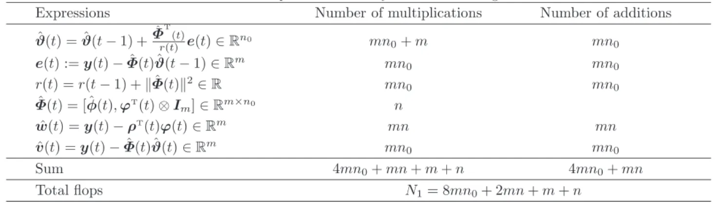
rise to a heavy computational burden. This motivates us to study some new identification algorithms to decrease the computational cost. For ease of comparison, the computational efficiency of the M-GESG algorithm at each recursive step is shown in Table 1, where flops represent the floating point operations.
Table 1: The computational efficiency of the M-GESG algorithm
Expressions Number of multiplications Number of additions
ˆ ϑ(t) = ˆϑ(t−1) +Φˆ T (t) r(t) e(t)∈Rn 0 mn 0+m mn0 e(t) :=y(t)−Φ(ˆ t)ˆϑ(t−1)∈Rm mn 0 mn0 r(t) =r(t−1) +kΦ(ˆ t)k2∈R mn 0 mn0 ˆ Φ(t) = [ ˆφ(t),ϕT (t)⊗Im]∈Rm×n0 n ˆ w(t) =y(t)−ρT (t)ϕ(t)∈Rm mn mn ˆ v(t) =y(t)−Φ(ˆ t)ˆϑ(t)∈Rm mn 0 mn0 Sum 4mn0+mn+m+n 4mn0+mn Total flops N1= 8mn0+ 2mn+m+n
4. The partially coupled generalized extended stochastic gradient algorithm
In this section, a partially coupled generalized extended stochastic gradient (PC-GESG) algorithm is derived by employing the decomposition technique and the coupling concept. The basic idea is to divide the multivariable identification model in (6) intomsubsystems, and to identify each subsystem based on the coupled relations in the part of parameters between subsystems.
Rewrite the hierarchical identification model in (6) for the M-CARARMA system in (3) as
y(t) =φ(t)β+ρT
ϕ(t) +v(t). (18)
LetφT
i(t)∈R1
×(nc+nd) be theith row of the information matrixφ(t):
φ(t) := [φ1(t),φ2(t),· · · ,φm(t)]
T
∈Rm×(nc+nd)
.
Similarly, letρi(t)∈Rnbe the ith column of the parameter matrixρ, that is
ρ:= [ρ1,ρ2,· · ·,ρm]∈Rn
×m.
By using the above definitions, Equation (18) can be rewritten as y1(t) y2(t) .. . ym(t) = φT 1(t) φT 2(t) .. . φT m(t) β+ ρT 1 ρT 2 .. . ρT m ϕ(t) + v1(t) v2(t) .. . vm(t) . (19)
Then we can decompose (19) into msubsystem identification models: yi(t) =φ T i(t)β+ρ T iϕ(t) +vi(t) =φT i(t)β+ϕ T (t)ρi+vi(t) = [φT i(t),ϕ T (t)] β ρi +vi(t), i= 1,2,· · ·, m. (20)
Define the subsystem information vector
ψi(t) := φi(t) ϕ(t) ∈Rn1 , n1:=n+nc+nd.
Equation (20) can be expressed as yi(t) =ψ T i(t) β ρi +vi(t), i= 1,2,· · ·, m. (21)
This is the subsystem identification model. From (21), we can see that each subsystem identification model contains the same parameter vectorβ and the same information vectorϕ(t).
Based on the subsystem identification models in (21), using the negative gradient search gives
ˆ β(t) ˆ ρi(t) = ˆ β(t−1) ˆ ρi(t−1) +ψi(t) ri(t) yi(t)−ψ T i(t) ˆ β(t−1) ˆ ρi(t−1) , (22) ri(t) =ri(t−1) +kψi(t)k2, ri(0) = 1, i= 1,2,· · · , m. (23)
Here, some problems arise. The first problem is that the subsystem information vectorψi(t), i= 1,2,· · ·, m, contains the unknown variablesw(t−j) andv(t−j). Similarly, we use the auxiliary models’ outputs ˆw(t−j) and ˆv(t−j) to replacew(t−j) andv(t−j) and construct the estimate ofφ(t):
ˆ
φ(t) := [−w(ˆ t−1),−w(ˆ t−2),· · ·,−w(ˆ t−nc),v(ˆ t−1),v(ˆ t−2),· · · ,v(ˆ t−nd)]
= [ ˆφ1(t),φˆ2(t),· · ·,φˆm(t)]
T
∈Rm×(nc+nd),
Define the estimate ofψi(t) by using ˆφi(t) andϕ(t):
ˆ ψi(t) := ˆ φi(t) ϕ(t) ∈Rn1×1 .
Based on (4)–(5), the estimates ˆw(t) and ˆv(t) can be calculated by ˆ w(t) =y(t)−ρˆT (t)ϕ(t), ˆ v(t) =w(t)−φˆ T (t)ˆβ(t) =y(t)−ρˆT (t)ϕ(t)−φˆT(t)ˆβ(t).
The second problem is that each subsystem has the same parameter vectorβ. That is to say, each subsystem can obtain the estimate ˆβ(t) of β. In order to make it clear, ˆβi(t) represents the estimate of Subsystem i. Replacing the unknown information vectorψi(t) with its estimate ˆψi(t) and the common parameter estimation vector ˆβ(t) with ˆβi(t) in (22)–(23), we have
ˆ βi(t) ˆ ρi(t) = ˆ βi(t−1) ˆ ρi(t−1) +ψˆi(t) ri(t) yi(t)−ψˆ T i(t) ˆ βi(t−1) ˆ ρi(t−1) , (24) ri(t) =ri(t−1) +kψˆi(t)k2. (25)
As we can see, there are estimates ˆβ1(t), ˆβ2(t), · · ·, ˆβm(t) for i = 1,2,· · · , m. In fact, we only need one
parameter estimate of β. In general, the parameter estimates approach their true values with the time t increasing. One may consider that the parameter estimate ˆβi−1(t) is closer to the true parameter than the parameter estimate ˆβi(t−1). Based on the coupling identification concept, for i= 1, use ˆβm(t−1) to replace
ˆ
β1(t−1), fori= 2,3,· · ·, m, use ˆβi−1(t) to replace ˆβi(t−1). Through the substitutions, we can obtain the
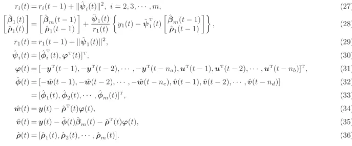
PC-GESG algorithm: ˆ βi(t) ˆ ρi(t) = ˆ βi−1(t) ˆ ρi(t−1) +ψˆi(t) ri(t) yi(t)−ψˆ T i(t) ˆ βi−1(t) ˆ ρi(t−1) , (26)
ri(t) =ri(t−1) +kψˆi(t)k 2, i= 2,3,· · · , m, (27) ˆ β1(t) ˆ ρ1(t) = ˆ βm(t−1) ˆ ρ1(t−1) +ψˆ1(t) r1(t) y1(t)−ψˆ T 1(t) ˆ βm(t−1) ˆ ρ1(t−1) , (28) r1(t) =r1(t−1) +kψˆ1(t)k2, (29) ˆ ψi(t) = [ ˆφTi(t),ϕT (t)]T , (30) ϕ(t) = [−yT (t−1),−yT (t−2),· · ·,−yT (t−na),u T (t−1),uT (t−2),· · ·,uT (t−nb)] T , (31) ˆ φ(t) = [−w(ˆ t−1),−w(ˆ t−2),· · ·,−w(ˆ t−nc),v(ˆ t−1),v(ˆ t−2),· · · ,v(ˆ t−nd)] (32) = [ ˆφ1(t),φˆ2(t),· · · ,φˆm(t)]T , (33) ˆ w(t) =y(t)−ρˆT (t)ϕ(t), (34) ˆ v(t) =y(t)−φ(ˆ t)ˆβm(t)−ρˆT (t)ϕ(t), (35) ˆ ρ(t) = [ˆρ1(t),ˆρ2(t),· · · ,ρˆm(t)]. (36)
The PC-GESG estimates are ˆβ(t) = ˆβm(t) and ˆρ(t)=[ˆρ1(t), ˆρ2(t), · · ·, ˆρm(t)]. So ˆβ(t) in the calculation of
ˆ
v(t) should be modified as ˆβm(t).
The steps involved in the PC-GESG algorithm in (26)–(36) are listed as follows.
1. Set the initial values: let t= 1, ˆβm(0) =1nc+nd/p0, ˆρi,0 =1n/p0, ri(0) = 1 (i = 1,2,· · ·, m), ˆw(0) =
1m/p0, ˆv(0) =1m/p0,p0= 106 and set a small positive numberǫ.
2. Collect the observation datay(t) andu(t), and construct the information matrixϕ(t) using (31). 3. Form ˆφ(t) using (32), read ˆφi(t) from (33), then construct ˆψi(t) by (30).
4. Computer1(t) using (29) and update the parameter estimates ˆβ1(t) and ˆρ1(t) using (28).
5. Fori= 2,3,· · ·, m, computeri(t) using (27) and update ˆβi(t) and ˆρi(t) using (26).
6. Form ˆρ(t) by (36), compute ˆw(t) and ˆv(t) using (34)–(35).
7. Compare ˆρ(t) with ˆρ(t−1) and compare ˆβm(t) with ˆβm(t−1): ifkϑ(ˆ t)−ϑ(ˆ t−1)k> ǫandkϑ(ˆ t)−ϑ(ˆ t−1)k> ǫ, increaset by 1 and go to Step 2; otherwise, terminate recursive calculation procedure and obtain ˆρ(t) and ˆβ(t) = ˆβm(t).
The schematic diagram of the PC-GESG algorithm in (26)–(36) is shown in Figure 1.
-ˆ βm−1(t) Subsystemm ? ym(t) ? ˆ ρm(t−1) ? ˆ ρm(t) ˆ βm(t) ppp Subsystem 2 ? y2(t) ? ˆ ρ2(t−1) ? ˆ ρ2(t) -ˆ β2(t) -ˆ βm(t−1) Subsystem 1 ? y1(t) ? ˆ ρ1(t−1) ? ˆ ρ1(t) -ˆ β1(t)
Figure 1: The schematic diagram of the PC-GESG algorithm
From Figure 1, we can see that only part parameters are coupled, that is to say, only ˆβi(t) are coupled between the subsystems, the parameter vectors ˆρi(t) are independent because each subsystem has a corresponding ˆρi(t).
This is the reason that we call this algorithm the partially coupled GESG algorithm.
Remark 4: Similarly, it is also reasonable to replacer1(t−1) withrm(t−1) and replaceri(t−1) (i= 2,3,· · ·, m)
withri−1(t). Then Equations (27) and (29) can be modified as
ri(t) =ri−1(t) +kψˆi(t)k
2, i= 2,3,· · ·, m, (37)
r1(t) =rm(t−1) +kψˆ1(t)k2. (38)
Then (26), (40), (28), (42) and (30)–(36) form another more complex PC-GESG algorithm. Here, the parameter βand the variabler(t) are coupled in the algorithm.
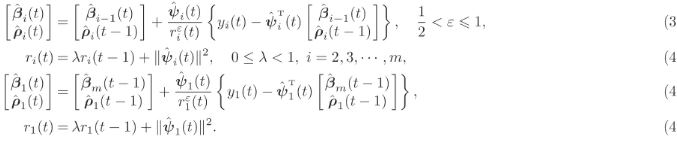
Remark 5: In order to improve the parameter estimation accuracy of the PC-GESG algorithm in (26)–(36), we can introduce the forgetting factorλin (27) and (29), or add the convergence indexεin (26) and (28):
ˆ βi(t) ˆ ρi(t) = ˆ βi−1(t) ˆ ρi(t−1) +ψˆi(t) rε i(t) yi(t)−ψˆ T i(t) ˆ βi−1(t) ˆ ρi(t−1) , 1 2 < ε61, (39) ri(t) =λri(t−1) +kψˆi(t)k2, 0≤λ <1, i= 2,3,· · ·, m, (40) ˆ β1(t) ˆ ρ1(t) = ˆ βm(t−1) ˆ ρ1(t−1) +ψˆ1(t) rε 1(t) y1(t)−ψˆ T 1(t) ˆ βm(t−1) ˆ ρ1(t−1) , (41) r1(t) =λr1(t−1) +kψˆ1(t)k2. (42)
Equations (26), (40), (28), (42) and (30)–(36) form the forgetting factor partially generalized extended stochastic gradient (GESG) algorithm. Combining (39)–(42) with (30)–(36), we can obtain the modified FF-PC-GESG (M-FF-PC-FF-PC-GESG) algorithm. When λ= 1 and ε= 1, the M-FF-PC-GESG algorithm reduces to the PC-GESG algorithm in (26)–(36).
Remark 6: The PC-GESG algorithm in (26)–(36) divides the MIMO system in (3) into m subsystems, and identifies the parameters based on the coupled relations between the subsystems. The computational efficiency of the PC-GESG algorithm is shown in Table 2.
Table 2: The computational efficiency of the PC-GESG algorithm
Expressions Number of multiplications Number of additions
"ˆ βi(t) ˆ ρi(t) # = " ˆ βi−1(t) ˆ ρi(t−1) # + ˆ ψi(t) ri(t)xi(t)∈R n1 mn 1+m mn1 xi(t) :=yi(t)−ψˆ T i(t) " ˆ βi−1(t) ˆ ρi(t−1) # ∈R mn1 mn1 ri(t) =ri(t−1) +kψˆi(t)k2∈R mn1 mn1 ˆ w(t) =y(t)−ρT (t)ϕ(t)∈Rm mn mn ˆ v(t) =y(t)−φ(ˆ t)ˆβm(t)−ρˆT (t)ϕ(t)∈Rm m(nc+nd) m(nc+nd) Sum 4mn1+m 4mn1 Total flops N2= 8mn1+m
In the M-GESG algorithm in (8)–(15), the dimension of the information matrix ˆΦ(t) is m×n0 (n0 =
nc+nd+mn). In the PC-GESG algorithm in (26)–(36), the dimension of the information matrix ˆψi(t) isn1×1
(n1=nc+nd+n). It is apparent from Tables 1–2 that the computational burden of the PC-GESG algorithm
is less than the M-GESG algorithm, that is to say, N1 ≫ N2. Compared with the M-GESG algorithm, the
PC-GESG algorithm avoids many redundant parameter estimates and improves the computational efficiency. Remark 7: This paper focuses on the parameter identification problems for multivariable CARARMA systems, which can be seen as an expansion to multivariable case of the CARARMA model in [26]. The multivariable CARMA-like model in [20] and [21] is another type of MIMO systems, which has the scalar polynomial in front of the output vectory(t). The PC-GESG algorithm proposed in this paper decompose the multivariable CARARMA system into m subsystems with the single output and identify each subsystem using the coupled relations between these subsystems. The work in [25] and [21] also used the hierarchical identification principle, but they divided the system into two parts and applied the least squares based iterative method to deal with the two parts. As for the estimation procedure, for every i, we get the estimate ˆρi(t). In order to obtain the
ˆ
βi(t), we use the estimate ˆβi−1(t) of Subsystemi−1 to replace the estimate ˆβi(t−1) of Subsystemi. Finally,
we can obtain ˆρ(t)=[ˆρ1(t), ˆρ2(t),· · ·, ˆρm(t)] and ˆβ(t) = ˆβm(t).
5. Examples
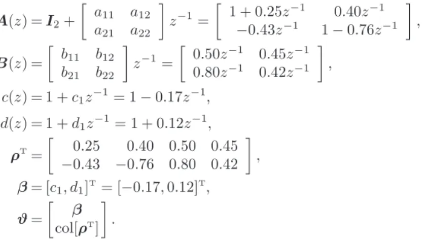
Example 1. Consider the following multivariable system with two-input two-output:
A(z)y(t) =B(z)u(t) +d(z)
A(z) =I2+ a11 a12 a21 a22 z−1= 1 + 0.25z−1 0.40z−1 −0.43z−1 1−0.76z−1 , B(z) = b11 b12 b21 b22 z−1= 0.50z−1 0.45z−1 0.80z−1 0.42z−1 , c(z) = 1 +c1z−1= 1−0.17z−1, d(z) = 1 +d1z−1= 1 + 0.12z−1, ρT = 0.25 0.40 0.50 0.45 −0.43 −0.76 0.80 0.42 , β= [c1, d1]T = [−0.17,0.12]T, ϑ= β col[ρT ] .
In simulation, the inputs {u1(t)} and {u2(t)} are taken as two independent persistent excitation signal
sequences with zero mean and unit variances,{v1(t)} and{v2(t)}are taken as two white noise sequences with
zero mean and variancesσ2
1 for v1(t) and σ22 forv2(t). Taking σ12=0.202,σ22=0.302, respectively, we use them
to generate the output vectory(t) = [y1(t), y2(t)]T. The parameter estimation error is in direct proportional to
the number of the parameters and the noise variance, and is in inverse proportion to the data length. Here, we choose the data lengtht= 3000 to estimate the parameters. To apply the M-GESG algorithm in (8)–(15), the PC-GESG algorithm in (26)–(36) and the FF-PC-GESG algorithm to estimate the parameters of this system, all the initial values of the parameters are set to be zero. The parameter estimates and errors are shown in Tables 3–5. The parameter estimation errorsδ:=kϑ(ˆ t)−ϑk/kϑkversust are shown in Figures 2–5.
Table 3: The M-GESG estimates and errors
t c1 d1 a11 a12 a21 a22 b11 b12 b21 b22 δ(%) 100 -0.06867 0.06610 0.05685 0.19915 -0.29108 -0.31399 0.30361 0.23460 0.37417 0.17876 52.51553 200 -0.08817 0.08414 0.06589 0.22001 -0.29961 -0.35736 0.31480 0.24555 0.39796 0.18911 48.68301 500 -0.10174 0.09510 0.08670 0.24658 -0.30398 -0.40209 0.33002 0.26416 0.42648 0.20727 44.14468 1000 -0.11188 0.10385 0.09795 0.26501 -0.30945 -0.43253 0.33982 0.27402 0.44760 0.22024 41.06893 2000 -0.12179 0.11170 0.10835 0.27978 -0.31164 -0.46424 0.34754 0.28500 0.46732 0.23182 38.18475 3000 -0.12704 0.11609 0.11397 0.28862 -0.31442 -0.48180 0.35245 0.29060 0.47988 0.23845 36.50561 True values -0.17000 0.12000 0.25000 0.40000 -0.43000 -0.76000 0.50000 0.45000 0.80000 0.42000
Table 4: The PC-GESG estimates and errors
t c1 d1 a11 a12 a21 a22 b11 b12 b21 b22 δ(%) 100 -0.12069 0.11019 0.12141 0.31966 -0.39648 -0.49910 0.46218 0.38248 0.52012 0.29075 29.19004 200 -0.13543 0.12283 0.13629 0.33369 -0.39808 -0.54744 0.46702 0.38959 0.55218 0.29628 25.22640 500 -0.14584 0.13040 0.16156 0.35161 -0.39697 -0.59295 0.47234 0.40259 0.58890 0.31626 20.67429 1000 -0.15145 0.13462 0.17440 0.36258 -0.39834 -0.61841 0.47483 0.40752 0.61324 0.32896 17.98801 2000 -0.15714 0.13883 0.18394 0.37035 -0.39634 -0.64536 0.47677 0.41339 0.63350 0.33989 15.62146 3000 -0.15941 0.14063 0.18898 0.37435 -0.39722 -0.65767 0.47811 0.41597 0.64644 0.34621 14.32294 True values -0.17000 0.12000 0.25000 0.40000 -0.43000 -0.76000 0.50000 0.45000 0.80000 0.42000
Table 5: The FF-PC-GESG estimates and errors (λ= 0.99)
t c1 d1 a11 a12 a21 a22 b11 b12 b21 b22 δ(%) 100 -0.13296 0.12033 0.13689 0.33229 -0.39721 -0.53841 0.47208 0.38619 0.54370 0.30444 25.79253 200 -0.15048 0.13510 0.16087 0.35064 -0.39951 -0.60660 0.47642 0.39826 0.59605 0.31322 19.97721 500 -0.16221 0.14222 0.21880 0.38224 -0.40065 -0.68726 0.48550 0.42655 0.68732 0.35863 10.47748 1000 -0.16548 0.14256 0.24410 0.40267 -0.41147 -0.72488 0.48764 0.43626 0.75133 0.39656 4.85150 2000 -0.17035 0.14634 0.24776 0.39674 -0.41453 -0.75299 0.49516 0.44617 0.78449 0.41986 2.35778 3000 -0.16843 0.14501 0.24977 0.39864 -0.42984 -0.76080 0.50236 0.44720 0.80790 0.42432 1.77632 True values -0.17000 0.12000 0.25000 0.40000 -0.43000 -0.76000 0.50000 0.45000 0.80000 0.42000
Example 2. Consider a following multivariable system:
A(z)y(t) =B(z)u(t) +d(z) c(z)v(t), A(z) =I2+ a1 a2 a3 a4 z−1+ a5 a6 a7 a8 z−2 = 1 + 0.52z−1−0.43z−2 0.45z−1+ 0.29z−2 −0.32z−1−0.24z−2 1−0.52z−1+ 0.48z−2 ,
0 500 1000 1500 2000 2500 3000 0 0.1 0.2 0.3 0.4 0.5 0.6 0.7 M−GESG PC−GESG FF−PC−GESG, λ = 0.99 t δ
Figure 2: The parameter estimation errors versust
0 500 1000 1500 2000 2500 3000 −0.8 −0.6 −0.4 −0.2 0 0.2 0.4 0.6 0.8 t Parameter estimates c 1 d 1 a 12 a 22 b 21
Figure 3: The M-GESG estimates ˆc1(t), ˆd1(t), ˆa12(t), ˆa22(t), ˆb21(t) versust
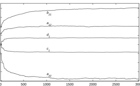
0 500 1000 1500 2000 2500 3000 −0.8 −0.6 −0.4 −0.2 0 0.2 0.4 0.6 0.8 t Parameter estimates c 1 d 1 a 12 a 22 b 21
0 500 1000 1500 2000 2500 3000 −0.8 −0.6 −0.4 −0.2 0 0.2 0.4 0.6 0.8 t Parameter estimates c 1 d 1 a 12 a 22 b 21
Figure 5: The FF-PC-GESG estimates ˆc1(t), ˆd1(t), ˆa12(t), ˆa22(t), ˆb21(t) versust
B(z) = b1 b2 b3 b4 z−1+ b5 b6 b7 b8 z−2= −0.10z−1−0.24z−2 0.26z−1−0.25z−2 0.67z−1+ 0.43z−2 0.26z−1+ 0.51z−2 , c(z) = 1 +c1z−1= 1 + 0.22z−1, d(z) = 1 +d1z−1= 1−0.17z−1, ρT = 0.52 0.45 −0.43 0.29 −0.10 0.26 −0.24 −0.25 −0.32 −0.52 −0.24 0.48 0.67 0.26 0.43 0.51 , β= [c1, d1]T= [0.22,−0.17]T, ϑ= β col[ρT ] .
Take the same simulation conditions as those in Example 1. Similarly, use the M-GESG algorithm, the PC-GESG algorithm and the FF-PC-GESG algorithm to estimate the parameters of this multivariable system, respectively. Since there are 18 parameters, we do not give the table for parameter estimates and errors. Here, we use the parameter estimation error curves to show the performance of the algorithms. The parameter estimation errors versustare shown in Figure 6.
0 500 1000 1500 2000 2500 3000 0 0.1 0.2 0.3 0.4 0.5 0.6 0.7 M−GESG PC−GESG FF−PC−GESG, λ = 0.99 t δ
Figure 6: The parameter estimation errors versust
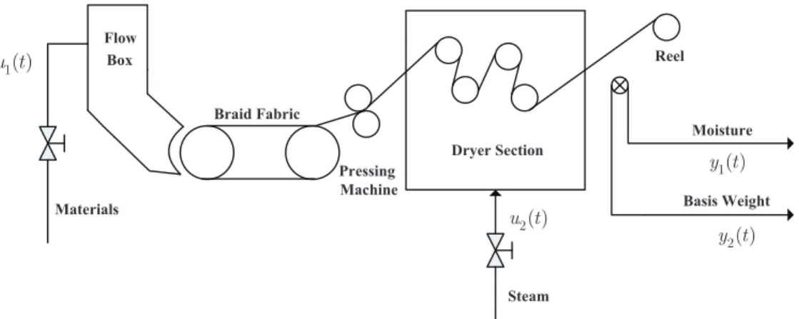
Example 3. The paper-making process can be viewed as a multi-input and multi-output stochastic system and can be modeled by a multivariable controlled autoregressive system. A simple sketch of the paper-making process is given in Figure 7. The thick paper fiber materials with a certain concentration from the pulp workshop
are pumped into a flow box to dilute them with water. After discharging from the flow box, the next step is to drain water from the materials by the braid fabric. Then the paper is formed by the pressing machine. The paper sheet goes through the dryer section to remove the remaining water by steam heating. Finally, workers check the moisture and basis weight of the manufactured paper and obtain the qualified products. By regulating the amount of the thick paper fiber materials and the steam pressure in the dryer section, the moisture and basis weight of the production can be controlled. In Figure 7,u1(t) and u2(t) are the amount of the materials
and the steam pressure,y1(t) andy2(t) are the moisture and the basis weight.
!"#$"%&$'()*+ &($,-.$$/ 0"$11)+2 3,'4)+$ 5",)6%7,8")' 3,($"),/1 u t1( )% 7/*9% 5*: 2( ) u t 1( ) y t 3*)1(;"$ 5,1)1%<$)24( 2( ) y t
Figure 7: A simple sketch of the paper-making process
Assume that the system fromu(t) toy(t) be modeled by the following multivariable model:
y(t) + −0.62 0.45 −0.58 −0.32 z−1y(t) + −0.33 0.29 −0.24 0.48 z−2y(t) = −0.86 0.16 0.68 −0.44 z−1 u(t) + −0.84 −0.65 0.55 0.61 z−2 u(t) +w(t),
wherew(t) is taken as an autoregressive moving average process of the white noise vectorv(t): w(t) =1 + 0.15z
−1−0.12z−2 1−0.12z−1+ 0.11z−2v(t).
The simulation conditions and steps are similar to those in Example 1. Takeλ= 0.9 and the data set length t = 3000. Apply the M-GESG, PC-GESG and FF-PC-GESG algorithms to estimate the parameters of this example system. Their estimation errorsδversustare shown in Figure 8.
0 500 1000 1500 2000 2500 3000 0 0.1 0.2 0.3 0.4 0.5 0.6 M−GESG PC−GESG FF−PC−GESG, λ = 0.9 t δ
Figure 8: The parameter estimation errors versust
1. The parameter estimation errors of the M-GESG, the PC-GESG and the FF-PC-GESG algorithms become smaller with the data lengthtincreasing – see the estimation errors of the last columns in Tables 3–5. 2. Under the same noise levels, the PC-GESG algorithm can give more accurate parameter estimates than
the M-GESG algorithm – see Tables 3–4 and Figures 2–6 and 8.
3. The FF-PC-GESG algorithm can improve the parameter estimation accuracy – see Table 5 and Figures 2, 6 and 8.
6. Conclusions
In this paper, we have presented a recursive identification algorithm of multivariable systems. This iden-tification algorithm has been developed for multivariable systems with autoregressive moving average noise. Differing from the M-GESG algorithm, the PC-GESG algorithm decomposes the original system into several subsystems according to the number of the outputs. The basic idea is to use the coupling concept to reduce the redundant parameter estimates of the coupled parameter vectors between subsystems. So the PC-GESG algorithm avoids the redundant computation and can improve the calculation efficiency. Through the numerical simulations, we can conclude that the PC-GESG algorithm has more accurate parameter estimates compared with the M-GESG algorithm. In addition, the FF-PC-GESG algorithm has smaller parameter estimation errors than the PC-GESG algorithm.
The differences between the previous identification algorithms and the PC-GESG algorithm are discussed. The presented algorithm is based on the decomposition technique and aimed to solve the coupled items between subsystems. The proposed coupling based identification method can be applied to other multivariable systems with different structures and disturbance noises. Moreover, the idea of this algorithm can be adopted when the concerned system model has the coupled terms. Applying the proposed algorithm to a real project will be further investigated in our future work. The proposed approaches in the paper can combine other mathematical tools [45, 46, 47] and statistical strategies [48, 49, 50, 51] to study the performances of some parameter estimation algorithms and can be applied to other multivariable systems with different structures and disturbance noises and other literature [52, 53, 54].
References
[1] Y. Wang, D. Zhao, Y. Li, S.X. Ding, Unbiased minimum variance fault and state estimation for linear discrete time-varying two-dimensional systems, IEEE Transactions on Automatic Control 62 (10) (2017) 5463-5469.
[2] Y. Wang, H. Zhang, S. Wei, D. Zhou, B. Huang, Control performance assessment for ILC-controlled batch processes in two-dimensional system framework, IEEE Transactions on Systems, Man and Cybernetics: Systems 48 (2018). doi: 10.1109/TSMC.2017.2672563 [3] W.H. Zhang, L. Xue, X. Jiang, Global stabilization for a class of stochastic nonlinear systems with SISS-like conditions and time delay,
International Journal of Robust and Nonlinear Control 28 (13) (2018) 3909-3926.
[4] Y. Li, W.H. Zhang, X.K. Liu, H-index for discrete-time stochastic systems with Markovian jump and multiplicative noise, Automatica 90 (2018) 286-293.
[5] S. Wu, W. Cui, Q. Shen, et al., Efficient parameter estimation method for maneuvering targets in discrete randomly-modulated radar, Digital Signal Processing 67 (2017) 91-106.
[6] L. Xu, F. Ding, Iterative parameter estimation for signal models based on measured data, Circuits, Systems and Signal Processing 37 (7) (2018) 3046-3069.
[7] L. Xu, The parameter estimation algorithms based on the dynamical response measurement data, Advances in Mechanical Engineering 9 (11) (2017) 1-12. doi: 10.1177/1687814017730003
[8] Y.J. Wang, F. Ding, L. Xu, Some new results of designing an IIR filter with colored noise for signal processing, Digital Signal Processing 72 (2018) 44-58.
[9] M.M. Mansouri, H.N. Nounou, M.N. Nounou, A.A. Datta, State and parameter estimation for nonlinear biological phenomena modeled by S-systems, Digital Signal Processing 28 (2014) 1-17.
[10] J. Na, G. Herrmann, K.Q. Zhang, Improving transient performance of adaptive control via a modified reference model and novel adaptation, International Journal of Robust and Nonlinear Control 27 (8) (2017) 1351-1372.
[11] M. Gan, C.L.P. Chen, G.Y. Chen, L. Chen, On some separated algorithms for separable nonlinear squares problems, IEEE Transactions on Cybernetics (2018). doi: 10.1109/TCYB.2017.2751558
[12] J. Na, J. Yang, X. Wu, et al, Robust adaptive parameter estimation of sinusoidal signals, Automatica 53 (2015) 376-384.
[13] J. Na, J. Yang, X.M. Ren, et al, Robust adaptive estimation of nonlinear system with time-varying parameters, International Journal of Adaptive Control and Signal Processing 29 (8) (2015) 1055-1072.
[14] L. Xu, F. Ding. Parameter estimation for control systems based on impulse responses, International Journal of Control, Automation, and Systems 15 (6) (2017) 2471-2479.
[15] L. Torres, J.F. G´omez-Aguilar, J. Jim´enez, et al., Parameter identification of periodical signals: Application to measurement and analysis of ocean wave forces, Digital Signal Processing 69 (2017) 59-69.
[16] M. Gan, H.X. Li, H. Peng, A variable projection approach for efficient estimation of RBF-ARX model, IEEE Transactions on Cyber-netics 45 (3) (2015) 462-471.
[17] X.R. Jing, A. Li, H.Q. Liu, A low-complexity Lanczos-algorithm-based detector with soft-output for multiuser massive MIMO systems, Digital Signal Processing 69 (2017) 41-49.
[18] J. Pan, H. Ma, X. Jiang, et al., Adaptive gradient-based iterative algorithm for multivariate controlled autoregressive moving average systems using the data filtering technique, Complexity 2018, Article ID 9598307. https://doi.org/10.1155/2018/9598307
[19] C.W.R. Chiong, Y. Rong, Y. Xiang, Blind channel estimation and signal retrieving for MIMO relay systems, Digital Signal Processing 52 (2016) 35-44.
[20] D.Q. Wang, Y.P. Gao, Recursive maximum likelihood identification method for a multivariable controlled autoregressive moving average system, IMA Journal of Mathematical Control and Information 33 (4) (2016) 1015-1031.
[21] H.Q. Han, L. Xie, F. Ding, X.G. Liu, Hierarchical least squares based iterative identification for multivariable systems with moving average noises, Mathematical and Computer Modelling 51 (9-10) (2010) 1213-1220.
[22] P. Ma, F. Ding, Q.M. Zhu, Decomposition-based recursive least squares identification methods for multivariate pseudolinear systems using the multi-innovation, International Journal of Systems Science 49 (5) (2018) 920-928.
[23] J.L. Ding, The hierarchical iterative identification algorithm for multi-input-output-error systems with autoregressive noise. Complex-ity, 2017, 1-11. Article ID 5292894. doi: https://doi.org/10.1155/2017/5292894
[24] J.L. Ding, Recursive and iterative least squares parameter estimation algorithms for multiple-input-output-error systems with autore-gressive noise, Circuits, Systems and Signal Processing 37 (5) (2018) 1884-1906.
[25] G.Y. Yao, R. Ding, Two-stage least squares based iterative identification algorithm for controlled autoregressive moving average (CARMA) systems, Computers & Mathematics with Applications 63 (5) (2012) 975-984.
[26] W. Wang, F. Ding, J.Y. Dai, Maximum likelihood least squares identification for systems with autoregressive moving average noise, Applied Mathematical Modelling 36 (5) (2012) 1842-1853.
[27] F. Ding, Y.J. Wang, J.Y. Dai, Q.S. Li, Q.J. Chen, A recursive least squares parameter estimation algorithm for output nonlinear autoregressive systems using the input-output data filtering, Journal of the Franklin Institute 354 (15) (2017) 6938-6955.
[28] X. Zhang, L. Xu, F. Ding, T. Hayat, Combined state and parameter estimation for a bilinear state space system with moving average noise, Journal of the Franklin Institute 355 (6) (2018) 3079-3103.
[29] L. Xu, W.L. Xiong, A. Alsaedi, T. Hayat, Hierarchical parameter estimation for the frequency response based on the dynamical window data, International Journal of Control, Automation and Systems 16 (4) (2018) 1756-1764.
[30] S.S. Cheng, Y.H. Wei, D. Sheng, et al., Identification for Hammerstein nonlinear ARMAX systems based on multi-innovation fractional order stochastic gradient, Signal Processing 142 (2018) 1-10.
[31] Y.J. Wang, F. Ding, A filtering based multi-innovation gradient estimation algorithm and performance analysis for nonlinear dynamical systems, IMA Journal of Applied Mathematics 82 (6) (2017) 1171-1191.
[32] L. Xu, F. Ding, Y. Gu, A. Alsaedi, T. Hayat, A multi-innovation state and parameter estimation algorithm for a state space system with d-step state-delay, Signal Processing 140 (2017) 97-103.
[33] Y. Cao, P. Li, Y. Zhang, Parallel processing algorithm for railway signal fault diagnosis data based on cloud computing, Future Generation Computer Systems 88 (2018) 279-283.
[34] Y. Cao, L.C. Ma, S. Xiao, et al., Standard analysis for transfer delay in CTCS-3, Chinese Journal of Electronics 26 (5) (2017) 1057-1063. [35] Y. Cao, Y. Wen, X. Meng, W. Xu, Performance evaluation with improved receiver design for asynchronous coordinated multipoint
transmissions, Chinese Journal of Electronics 25 (2) (2016) 372-378.
[36] Y.Z. Zhang, Y. Cao, Y.H. Wen, L. Liang, F. Zou, Optimization of information interaction protocols in cooperative vehicle-infrastructure systems, Chinese Journal of Electronics 27 (2) (2018) 439-444.
[37] X. Zhang, F. Ding, F.E. Alsaadi, T. Hayat, Recursive parameter identification of the dynamical models for bilinear state space systems, Nonlinear Dynamics 89 (4) (2017) 2415-2429.
[38] M.T. Chen, F. Ding, L. Xu, T. Hayat, A. Alsaedi, Iterative identification algorithms for bilinear-in-parameter systems with autore-gressive moving average noise, Journal of the Franklin Institute 354 (17) (2017) 7885-7898.
[39] J. Pan, X. Jiang, X.K. Wan, et al., A filtering based multi-innovation extended stochastic gradient algorithm for multivariable control systems, International Journal of Control, Automation, and Systems 15 (3) (2017) 1189-1197.
[40] X. Zhang, F. Ding, L. Xu, E.F. Yang, State filtering-based least squares parameter estimation for bilinear systems using the hierarchical identification principle, IET Control Theory and Applications 12 (12) 1704-1713.
[41] F. Ding, H.B. Chen, L. Xu, J.Y. Dai, Q.S. Li, T. Hayat, A hierarchical least squares identification algorithm for Hammerstein nonlinear systems using the key term separation, Journal of the Franklin Institute 355 (8) (2018) 3737-3752.
[42] F. Ding, Coupled-least-squares identification for multivariable systems, IET Control Theory and Applications 7 (1) (2013) 68-79. [43] F. Ding, D.D. Meng, J.Y. Dai, Q.S. Li, A. Alsaedi, T. Hayat, Least squares based iterative parameter estimation algorithm for stochastic
dynamical systems with ARMA noise using the model equivalence, International Journal of Control, Automation and Systems 16 (2) (2018) 630-639.
[44] F. Ding, L. Xu, F.E. Alsaadi, T. Hayat, Iterative parameter identification for pseudo-linear systems with ARMA noise using the filtering technique, IET Control Theory and Applications 12 (7) (2018) 892-899.
[45] F. Liu, H.X. Wu, Singular integrals related to homogeneous mappings in triebel-lizorkin spaces, Journal of Mathematical Inequalities 11 (4) (2017) 1075-1097.
[46] F. Liu, H.X. Wu, Regularity of discrete multisublinear fractional maximal functions, Science China–Mathematics 60 (8) (2017) 1461-1476.
[47] F. Liu, H.X. Wu, On the regularity of maximal operators supported by submanifolds, Journal of Mathematical Analysis and Applica-tions 453 (1) (2017) 144-158.
[48] C.C. Yin, C.W. Wang, The perturbed compound Poisson risk process with investment and debit interest, Methodology and Computing in Applied Probability 12 (3) (2010) 391-413.
[49] C.C. Yin, K.C. Yuen, Optimality of the threshold dividend strategy for the compound Poisson model, Statistics & Probability Letters 81 (12) (2011) 1841-1846.
[50] C.C. Yin, Y.Z. Wen, Exit problems for jump processes with applications to dividend problems, Journal of Computational and Applied Mathematics 245 (2013) 30-52.
[51] C.C. Yin, Y.Z. Wen, Optimal dividend problem with a terminal value for spectrally positive Levy processes, Insurance Mathematics & Economics 53 (3) (2013) 769-773.
[52] P.C Gong, W.Q. Wang, F.C. Li, H. Cheung, Sparsity-aware transmit beamspace design for FDA-MIMO radar, Signal Processing 144 (2018) 99-103.
[53] Z.H. Rao, C.Y. Zeng, M.H. Wu, et al., Research on a handwritten character recognition algorithm based on an extended nonlinear kernel residual network, KSII Transactions on Internet and Information Systems 12 (1) (2018) 413-435.
[54] N. Zhao, R. Liu, Y. Chen, M. Wu, Y. Jiang, W. Xiong, C. Liu. Contract design for relay incentive mechanism under dual asymmetric information in cooperative networks, Wireless Networks (2018). doi: 10.1007/s11276-017-1518-x