Symmetrically normalized instrumental-variable estimation using panel data.

Working Paper 96-45

Statistics and Econometrics Series 16 July, 1996

Departamento de Economía Universidad Carlos III de Madrid Calle Madrid, 126 28903 Getafe (Spain) Fax (341) 624-98-75

SYMMETRICALLy NORMALIZED INSTRUMENT AL-VARIABLE ESTIMATION USING PANEL DATA

César Alonso-Borrego * and Manuel Arellano ••

Abstract _ _ _ _ _ _ _ _ _ _ _ _ _ _ _ _ _ _ _ _ _ _ _ _ _ _ _ _ _ _ __ In this paper we discuss the estimation of panel data models with sequential moment restrictions using symmetrically normalized GMM estimators. These estimators are asymptotically equivalent to standard GMM but are invariant to normalization and tend to have a smaller finite sample bias. They also have a very different behaviour compared to standard GMM when the instruments are poor. We study the properties of SN-GMM estimators in relation to GMM, minimum distance and pseudo maximum likelihood estimators for various versions of the AR(1) model with individual effects by mean of simulations. The emphasis is not in assessing the value of enforcing particular restrictions in the model; rather, we wish to evaluate the effects in small samples of using alternative estimating criteria that produce asymptotically equivalent estimators for fixed T and large N. Finally, as an empírical illustration, we estimate by SN-GMM employment and wage equations using panels of UK and Spanish firms.

Keywords: Panel data, instrumental variables, symmetric normalization, autoregressive models, employment equations.

• Departamento de Economía, Departamento de Estadística y Econometría de la Universidad Carlos III de Madrid .•• CEMFI, Madrid

We thank Richard Blundell, Gary Chamberlain, Guido Imbens, Whitney Newey, Enrique Sentana, Jim Stock an seminar audiences at Harvard, Princeton and Northwestern for useful comments. An earlier version of this paper was presented at the ESRC Econometric Study Group Annual

1. Introduction

In this paper we present instrumental variable estimators of panel data models with predetermined variables subject to a symmetric normalization rule of the coefficients of the endogenous variables. We also evaluate the performance of these techniques for first-order autoregressive models with individual effects by mean of simulations. Lastly, an empirical illustration is provided.

This work is motivated by a concern with the biases of ordinary IV estimators when the instruments are poor. A linear panel data model wl th predetermined variables, typically estlmated by IV techniques,

takes the form

E(Lly - Llx' <5 z .. z ) = O, (t=1, .. ,T; i=1, .. ,N). i t i t 11 i t

This formulation includes vector autoregressions and linear Euler equations. The specification of the equation error in first­ differences reflects the fact that the analysis is conditional on an unobservable individual effect. Since the number of instruments increases with T, the model generates many overidentifying restrictions even for moderate values of T. However, often the quality of the instruments is poor given that it is usually difficult to predict variables in first differences on the basis of past values of other variables.

The weaker the correlation of the instruments with the endogenous variables, the smaller the amount of information on the structural parameters for a given sample size. However, as it is well documented in the literature on the finite sample properties of simultaneous

equations estimators, the way in which this situation is reflected in the distributions of 2SLS and LIML differs substantially, despite the fact that both estimators have the same asymptotic distribution. While the distribution of LIML is centred at the parameter value, 2SLS is biased towards OLS, and in the completely unidentified case converges to a random variable with the OLS probabili ty limit as its central value. On the other hand, LIML has no finite moments regardless of the sample size, and as a consequence its distribution has thicker tails than that of 2SLS and a higher probability of extreme values (see Phlllips (1983) for a good survey of the literature). As a result of numerical comparisons of the two distributions involving median-bias, interquartile ranges and rates of approach to normali ty, Anderson, Kunitomo and Sawa (1982) conclude that LIML is to be strongly preferred to 2SLS, particularly if the number of outside lnstruments is large. Similar conclusions emerge from the results of asymptotic approximations based on an increasing number of instruments as the sample size tends to lnfini ty; under these sequences, LIML is a conslstent estimator but 2SLS is inconslstent (cf. Kunitomo (1980), Morimune (1983) ando more recently, Bekker (1994)).1 (In our contexto these approximations would amount to allowlng T to increase to inflnlty at a chosen rate as opposed to the standard flxed T, large N asymptotics. )

Despite this favourable evidence. LIML has not been used as much in applications as instrumental variables estimators. In the past, LIML was at a disadvantage relative to 2SLS on computational grounds. More fundamentally, applied econometric1ans have often regarded 2SLS as a more "flexible" choice than LIML from the point of vlew of the

restrictions they were will1ng to impose on their models. In effect, the IV techniques used for a panel data model wi th predetermined instruments are not standard 2SLS estimators, since the model gives rise to a system of equations (one for each time period) wi th a different number of instruments available for each equation. Moreover, concern with heteroskedasticity has lead to consider alternative GMM estimators that use as weighting matrix more robust estimators of the variances and covariances of the orthogonal1 ty condi tions (following the work of Chamberlain (1982), Hansen (1982) and White (1982)).

In a recent paper, Hillier (1990) shows that the alternative normalization rules adopted by LIML and 2SLS are at the root of their different sampling behaviour. Indeed, Hill1er shows that the symmetrically normalized 2SLS estimator (SN-2SLS) has essentially similar properties to those of the LIML estimator. This result, which motivates our focus on symmetrically normalized estimation, is interesting because SN-2SLS, unlike LIML, is a GMM estimator based on structural form orthogonality conditions and therefore it can be readily extended to the nonstandard IV situations that are of interest in panel data models wi th predetermined variables, while relying on standard GMM asymptotic theory.

To illustrate the situation, let us consider a simple structural equation with a single endogenous explanatory variable and a matrix of instruments Z:

y

=

(3x + u (1.1)

.equations y

=

Zn + v 1 (1. 2) X

=

Zr

+ v 2

the 2SLS est1mator of ~ 1s g1ven by

"

=

Cov(x:y ) Cov(x,y)

== A

~2SLS

Var(x) COV(X,X)

which is not invariant to normal1zation except 1n the just-identified case. That 15, it differs from the indirect 2SLS estimator:

...

"

=

Var(y) Cov(y.y)

~I2SLS

"

Cov(y,x) Cov{y,x)

On the other hand, the SN-2SLS estimator is given by the orthogonal regression of Y on x, which is invariant to normalization:

" ... = Cov(x,y) Var(y)-I\.

==

---;:~-~SN ... "

Var(x)-I\. Cov(y,x)

The stat1stic 1\. is the minimum eigenvalue of the covariance matrix of y and x.

The three estimators have the same first-order asymptotic distribution, but satisfy the inequality

Moreover, ~SN can be written as COy (x+~ y, y) SN ~SN

=

A " " Cov(x+~ y.x) SN

Therefore. 2SLS, I2SLS and SN can al! be interpreted as simple IV

estimators that use as instruments x,y and x + ~ y. respectively.

SN

Symmetrically normalized 2SLS can also be given a straightforward interpretation as a GMM or minimum distance estimator. which highlights its relation to LIML. Indeed, both SN-2SLS and LIML are least-squares estimators of the reduced form (1.2) imposing the over­ identifying restrictions n=~r. Let us define

(~

.1 )

=

argmin

[y-zr~l'

(V-1®I)

[y-zr~l

v v x-Zr x-Zr

~.r

Concentrating r out of the LS criterion we obtain

~v

=

argmin ~

It turns out that LIML is

-

~ with V equal to the reduced form v

'1

identity matrix (cf. Malinvaud (1970), Goldberger and Olkin (1971) and Keller (1975», so that both LIML and SN-2SLS solve minimum eigenvalue problems. In particular, SN-2SLS is a GMM estimator based on the unit­ length orthogonality conditions

Notice that in spite of V being a matrix scaling factor, the asymptotic distributlon of ~ does not depend on the choice of V. This

v

,..

is so because optimal MD estimators of ~ based on (n-1~,1-1) and on ,..

(n-1~) are asymptotically equivalent, due to the fact that the limi ting distribution of opt1mal MD 1s invar1ant to transformations and to the add1tion of unrestricted moments.

The paper is organized as follows. Section 2 begins with a formulation of the SN-2SLS estimator and its relation to 2SLS and LIML in the general context of a linear structural equation. Next, we present two-step SN-GMM estimators and test statistics of over­ identifying restrictions for panel data models with predetermined instruments. Section 3 studies the finite sample properties of SN-GMM estimates in relation to ordinary GMM. minimum distance and pseudo maximum likelihood estimators for various versions of the first-order autoregress1ve model with individual effects. The objective is not to assess the value of enforcing particular restrictions in the model, but rather to evaluate the effects in small samples, by mean of simulations, of using alternative asymptotically equlvalent estimators for fixed T and large N. Section 4 re-estimates the employment

equations for a sample of UK firms reported by Arellano and Bond (1991) using symmetrically normalized and indirect GMM estimators. This section further illustrates the techniques by presenting SN-GMM estimates and bootstrap confidence lntervals of employment and wage vector autoregresslons from a larger panel of Spanlsh flrms. Flnally, Section 5 contalns the conclusions of the paper.

2. The Symmetrically Normalized Instrumental-Variable Estimator

Preliminaries

We begin this section by providing explicit express10ns for 2SLS, LIML and symmetrically normalized 2SLS estimators in order to highlight the algebraic and statistical connections among the three statistics.

Let us cons1der a standard linear structural equation

y =

y

~ +

z

o + u

=

Xo

+ u. (2.1 )

1 2 1

Also let Y=(y ,Y ) be the nx(l+p) matrix of observations of the

1 2

endogenous variables, and let Z=(Z ,Z) be the nxk matr1x of 1 2

1nstruments, where Z is nxk ,Z 1s nxk , and k ~p.

1 1 2 2 2

The two-stage least squares (2SLS) estimator of

o

1s given by

o

= argmin a'W'MWa (2.2)

2SLS

_o

wlth W=(Y,Z), M=ZeZ'Z)-lZ' and a=(l.-~· ,-o')'. An expression for the 1

partition of

o

is given by

= argmin b'Y' (M-M )Yb = [Y' (M-M )Y ]-ly ' (M-M )y

(32SLS _{2 1 2 2 1 1}

(3 1

with b=(1, -(3' )' and M =Z (Z' Z)-1Z'. 1 1 1 1 1

Similarly, the LIML estimator is given by

a'W'MWa

(3 _{= argmin " = [X' (M-i(I-M)/n)X]-I X' (M-i(I-M)/n)y (2.3)}

LIML _{(3 b'Qb} 1

where A=min eigen[Y' (M-M )YQ₁ "-1 ] and Q=Y' (I-M)Y/n, which can be partitioned in accordance with Y as

A

Notice that A~O. Equally,

b' Y' (M-M )Yb

=

argmin _ _~,,_1_ _

=

[Y' (M-M )Y -ic ]-1 [Y' (M-M )y -i~ ]

(3LIML _{(3 b' Qb 2 1 2 22 2 1 1 21}

We define the orthogonal or symmetrically normalized 2SLS estimator (SN-2SLS) to be (see Keller (1975) and Hillier (1990»:

• •

••

•

•

a'W'M'Wa

°

= argmin - - - - ; ; - ¡ - ; - - (2.4) SNM

°

Let Wa =Yb +2 c =u denote equation (2.1) without imposing a 1

•

normal1zatlon rule. With the normal1zatlon used by 2SLS a =a, while with a symmetric normalization of the coefficients of the endogenous variables a• _{=O+{3' (3)} -1/2_{a. Thus} 0SNM is the minimizer of a'• _{W' M'Wa}• subject to b 'b =1.

Minimizing the criterion (2.4) with respect to r we obtain a concentrated criterion that only depends on {3. This gives us:

b' Y' (M-M )Yb 1 = argmin - - - - C

b'""'''b--

=

[y; (M-M )Y1 2 -

~Il-1y;

(M-M1)Y1 {3

= (2'2 )-1_{2 , (y} -y ~ ) 1 1 1 1 2 SNM

where A=min eigen[Y' (M-M )Yl. Notice that also A=min(a'W'M'Wa)/b'b and 1

that A~O. Equivalently,

(2.5)

where

~

=

[~ ~

l.

A

In the just identified case, 2' (y -Xo )=0 which min1mizes the 1 2SLS

three criteria, so that A=A=O, with the result that 2SLS, LIML and SN­ 2SLS coincide.

Both 0LIML and 0SNM are invariant to norma11zation while 02SLS is noto 2 That is, if the equation 1s solved for an endogenous variable other than Y1' contrary to the case with 2SLS, the indirect estimates

obtained from

o

_SNM or

o

_LIML coincide wi th .the direct SNM' or LIML estimates, respectively.3

The LIML estlmator can be regarded as a minimum distance or generallzed nonlinear least squares estlmator based on the reduced form (see Malinvaud (1970) and Goldberger and Olkin (1971)). Similarly, the SN-2SLS estimator can be viewed as an ordinary nonlinear least squares estimator. To see this, let the reduced form of

Y

be

y

=

ZTI' + V. _(2.6)

In view of the partition in Y, the (l+p)xk matrix of reduced form coefficients can be partitioned as TI'={n , TI;). In addition, given the

1 structural equation we have

n~

=

~'TI2 + (o' ,0' ) _(2.7)

so that TI is a function of ~,

o

and TI • We can consider NLS estimators 2

of

o

and TI that solve 2

(o TI ) - argmin tr[V-1 (Y-ZTI' )' (Y-ZTl' )] _(2.8)

NLS' 2,NLS ­

for particular choices of V. This class of estimators was proposed by Keller (1975). Since TI is not of direct interest we can obtain a

2

concentrated NLS criterion that only depends on

o,

which gives 0NLS as the solutlon to

a'W'MWa

es

_NLS = argmin b' Vb . (2.9)

Clearly, LIML is

es

NLS with V=O whlle SN-2SLS is

es

NLS with V=I.

The choice of V, provided it is assumed to be bounded in probability ... or a nonstochastic matrix, leaves the asymptotic distribution of

es

NLS

unaffected and equal to that of the 2SLS estimator. This result is similar to the one that establishes the equivalence between 2SLS and 3SLS in a system in which there is only one overidentified structural equation.

Symmetrically normalized estimators are attractive alternatives to 2SLS on at least three grounds. Firstly, they tend to have a smaller finite sample bias than the 2SLS estimators. Hillier (1990) shows that for the normal case with p=l SN-2SLS and LIML are "spherically unbiased" in finite sainples. 4 _{However, 2SLS does not have}

this property.

Secondly, the concentration of the densities of the symmetrically normalized estimators depends on the quality of the instruments. In the completely unidentified case, as shown by Hillier, these estimators have a uniform distribution on the unit circle. This is in contrast with 2SLS which converges to the same llmlt as OLS and whose distribution is determined exclusively by the normalization adopted. When the instruments are poor, as well as when the number of

instruments is large relative to the sample size, 2SLS tends to provide results that are biased in the direction of OLS and also large discrepancies between "direct" and "indirect" 2SLS when using different normalizations. This situation has been stressed in a number of recent papers (Bekker (1994), Bound, Jaeger and Baker (1995»,

Staiger and stock (1994) and Angrist and Krueger (1995) amongst others). In contrast, with poor instruments the distributions of LIML and SN-2SLS accurately reproduce the fact that the information on the structural parameters is very small.

Thirdly, they are invariant to normalization. SN-2SLS shares these properties in common with LIML; however, one further advantage of SN-2SLS in relation to LIML, is that it is a generalized method of moments estimator based on structural form moment conditions and therefore it can be easily extended to distribution free environments and robust statlstlcs. In particular, i t is well sui ted for application to nonstandard instrumental-variable problems such as those that arise in the context of dynamic and error-in-variables models for panel data.

As the previous discussion reveals, both LIML and SN-2SLS are GMM estimators of

o

solved jointly with TI and based on the vector of the

2

reduced form orthogonality conditions:

(2.10)

where TI is a function of

o

and TI (both GMM estimators use a weighting 2

matrix of the form (V®Z' Z)-1 wi th

v=o.

" for LIML and V=I for SN-2SLS). However, SN-2SLS is also a GMM estimator of

o

based on the structural form orthogonality conditions:

(In the last two expressions, z, y, y and Xl refer to the i-th

1 1 11

rows of 2, Y, Y1 and X respectively.)

There is one disadvantage, however, of SN-2SLS relative to the other estimators.< In general, the results are not independent of the units in which the variables are measured, so that a sensible choice of the units of scale may be of sorne importance. 5

One further useful perspective on SN-2SLS can be obtained by regarding it as a simple IV estimator. The statistic h can be written as

"

h = y~ (M-M ) (Yl-XoSNM) 1

Substituting this express ion in the formula for the estimator we obtain

(2.12)

where

"

2

=

X + (M-M1)Y1o~NMd

which reduces to Z=X+y

o'

if all the variables in X are endogenous. 1 SNM

Remark that for 2SLS we have Z = X, and more generally for the j-th indirect 2SLS estimator obtained by normalizing to unity the coefficient on the j-th column of Y, we have 2=W(j) , where W(j)

"­ coincides w1th W=(Y. 2

1 ) except for the j-th column of Y which is omitted.

Models lor Panel Data

We consider a model with individual effects for panel data given by

= x' Ó + U _{(t=1 •...• T; i=1 •...• N) (2.13)}

1t lt

u = 1) + v 1t l I t

The model specifies sequential moment conditions of the form

E(v_lt

I

_(2.14)

were

z;=(zl~

'"

zl~)'

is a vector of instrumental variables.

Thus. this setting is sufficiently general to cover models with strictly exogenous. predetermined and endogenous explanatory variables. We assume that

i=1 •... N} is a random sample (iid) of size N.

Estimation will be based on a sequence of orthogonality conditions of the form

(t=1 •...• T-1) (2.15)

where starred variables denote forward differences or orthogonal deviations of the original variables (e.g. y;t=Yl(t+1)-Ylt)'

It is convenient to rewrite the transformed model in the form

y.

=

X·ó + u·

•

•

•

where y -(y _{1- 11 Y1 (T-1)} )' _, etc_•

The mx1 parameter vector

o

1s usually est1mated by GMM lead1ng to est1mators of the form (see Holtz-Eak1n, Newey and Rosen (1988), Arellano and Bond (1991), Chamberla1n (1992), Arellano and Bover

(1995), and Ahn and Schmidt (1995) amongst others):

(2.16)

where y.=(y.. ' ... y.')', X·=(X·' ... X·')' and 2=(2i ... 2

_N)'.

2₁ 1s a (T­

1 N 1 N

t

1 )xq block diagonal matrix whose t-th block is Z1' and AN 1s chosen such that it is a consistent estimate of the inverse of E(2'u·u·'2 J.

I I 1 1

The standard robust choice is

AN = (~ 2'u·u·'2 )-1

L.1 I I 1 1

where u· is a vector of residuals evaluated using some preliminary 1

consistent estimate of

o.

Under very general regularity conditions

.fN'(5

GHH-O) is asymptotically normal as

N~

and T is fixed, and a

consistent estimator of the asymptotic variance of

o

is g1ven by GHH

(X·'2 A 2' X·)-l (2.17)

N

Moreover, the Sargan or GMM statistic of overident1fylng restrlctlons is glven by

s

=

u·,

2 A 2'

u·

~

i

"

where u

".

= y

.

- X·á .

GHH

Turning to symmetrically normalized GMM (SNM) estimators of á, let us consider a partition of X·=(X· X·) _{and a corresponding}

l ' 2

parti tion of á=(á' á')' distinguishing between non-exogenous and_{l ' 2} exogenous variables, such that the m columns of X· are linear

2 2

combinations of those of Z while the m columns of X· are noto

1 1

SNM is the GMM estimator of á based on the orthogonality conditions Z' (y·-X ·á -X ·á )

1

E

1/1(1.1 ,á) = E 1 1 11 1 21 2

=

O _(2.18) 1 [ (1+á'á )1/2 1 1

Since E[I/1(w ,á)I/1'(w ,á)] = E(Z'u·u·'Z )/(l+á'á )=A l(l+á'á ) A

1 1 1 1 1 1 11 N 1 1 ' N

remains an optimal weighting matrix for the SNM estimator. Therefore,

(y·-X·á)'M·(y·-X·á)

á _{= argmin (l+á'á ) (2.19)}

SNH

á 1 1

where M· = ZA Z'. Following our earlier discussion we obtain N d'W·' (M·-M·)W·d 1 1 2 1 1 á _lSNH = argmin _d'd (2.20) 1 1 á ₁ (2.21)

where W· = (y. X·) d = (1 -á')' and M· = M·X·(X·'M·X·)-l X·'M·. So

1 ' 1 ' 1 ' 1 2 2 2 2 2

= [X·' (M·-M·)X· - AIl-1 _{X·, (M·-M·)y·}

(2.22)

1 2 1 1 2

wi th A

=

min eigen[W·' (M·-M·)W·]. A compact expression for o is

. 1 2 1 SNH

given by

o

=

(X·'M·X· - AÓ)-l X·'M·y· (2.23)

SNH

A A

Since O and O areasymptotically equi valent, Vado ) is

GMM SNM GMH

also a consistent estímate of the asymptotic varlance of O

SNH

A A

However, an alternatíve natural estímator of Vado ), suggested by

SNM

theexpresslon above, is

A "

Vareo )

=

(X·'M·X· - AÓ)-l (2.24)

SNM

Moreover, since A is a minlmized optimal GMM crlterion it can be used as an alternative test statistic of overidentifying restrictions. We have the result

(1 +

o'

o

)A ~

-l

(2.25)

lSNM lSNM q-m

which 1s asymptotically equivalent to the Sargan test.

The ex1sting evidence from Monte CarIo experiments and empirical analysis point in the direct10n that, even for moderately large cross­

sectional sample sizes, ordinary GMM estimates and their standard errors can be worryingly biased when the instruments are poor. This is typically the case in the context of autoregressive models with individual effects when the roots are close to unity or the contribution of the permanent effect to the total variance is high. If the desirable fini te sample properties of symmetrical1y normalized estimators apply to these environments, o , Var(o ) and A could

SNK SNM

provide a useful alternative to estimation and testing.

3. Experimental Comparisons with Alternative Estimators for First Order Autoregressions with Random Effects

The purpose of this section is to study the finite sample properties of the symmetrically normalized GMM estimators in relation to ordinary GMM for varIous versions of the first-order autoregressive model with Individual effects. The IV restrictions implled by these models can also be represented as simple structures on the covariance matrix of the data, and so we can also make comparisons with minimum distance and pseudo maximum likelihood estImators of these covariance structures. The emphasis is not in assessing the value of enforcing particular restrIctions in the model, as done for example by Ahn and Schmidt (1995) and Arellano and Bover (1995) for quadratic and stationarity restrictions, respectively. Rather, we wish to evaluate the effects in small samples of usIng alternative estimatIng criteria that produce asymptotically equivalent estimators for fixed T and large N. However, since we present results for three different sets of moment restrictions, we shall also be able to make some comparisons

across models. We concentra te on a random effects AR(l) model because of its simplicity and the fact that it is a case that has received a great deal of attention in the literature.

Hodels and Estimators

Let us consider a random sample of individual time-series of size T Y:=(Yl1, , .. 'Y1T)' (1=1"" ,N) with second-order moment matrix E(//' )=Q={w }. We assume that the joint distribution of

/1

and the

1 1 ts

unobservable time-invariant effect satisfies the following assumption:

Assumption A

Ylt = l' + "Y + 'V> + V (t=2, ... , T) (3.1)

1(t-1) "1 lt

(3.2)

Notice that since equation (3.1) includes a constant term, it is not restrictive to assume that 11 has zero mean. However, in general

1

T

E(11

_I

YT ) will be a function of Y ' Moreover, the dependence between 11

1 1 1 1

and v is not restricted by Assumption A. Another remark is that

lt

Assumption A does not rule out the possibility of conditional heteroskedasticity, since E(v~tly~-1) need not coincide with ~~.

Following Arellano and Bond (1991), Assumption A implies (T-2)(T­

(3.3)

These restrictions can also be represented as constraints on the elements of

n.

Multiplying (3.1) by Yls for s<t, and taking expectations gives:

w =aw +c (t=2, ... Ti s=l, ... ,t-l) (3.4)

ts (t-l)s s

where e =E[y (r+ij )]. This means that, given Assumption A, the

s 1s 1

T(T+l)/2 different elements of

n

can be writ ten as functions of the 2Txl parameter vector

We call this moment structure Model 1. Since the moment restrictions in (3.3) are linear in a, they can be used as the basis for a linear GMM estimator of the type discussed in the previous section.

The orthogonality conditions (3.3) are the only restrictions implied by Assumption A on the second-order moments of the data. 7 _In

particular, wi th T=3 the parameters (a, e ,e ) are just-identified as

1 2

functions of the elements of

n.

Model 1 is attractive because it is based on minimal assumptions. However, we may be wllling to impose addi tional structure i f this conforms to a priori bellefs. One possibility is to assume that the errors v a r e mean independent of the individual effect ij given

lt 1

Assumption B

(3.5)

Note that Assumption B is more restrictive than Assumption A. When T~4, Assumption B implies the following additional T-3 moment restrictions

In effect, we can write

E [ (y - 'Y - exy - 'n ) (lIy - exlly )]

=

O

1t a 1 (t-l) "1 Ut-l) Ut-2)

and since E[('1+r¡ )lIv ]=0 the result follows. GMM estimators of ex

1 1 (t-l)

that exploi t these restrictions inaddi tion to those in (3.3) have been considered by Ahn and Schmidt (1995). An alternative representation of the restrictions in (3.6) is in terms of a recursion of the coefficients c introduced in (3.5). Multiplying (3.1) by

t

('1+r¡ ) and taking expectations gives:

1

(t=2, ... ,T) (3.7)

where 4>=l+0'2=E[('1+r¡ )2], so that c ... c can be written in terms of

r¡ 1 1 T-1

C and 4>. This gives rise to Model 2 in which Q depends on the (T+3)x1

1

Notice that with T=3 Assumption B does not imply further restrictions in O with the result that a remains just identified relat1ve to the

second-order moments.

other forms of addit10nal structure that can be imposed are various versions of mean or variance stationarity condit10ns. Assumpt10n C. wh1ch requires the change in y

lt to be mean independent of the individual effect

T/ 1 • 1s a particularly useful mean stationarity condition.

Assumption

e

(t=2 •...• T) (3.8)

Notice that in combination with Assumption

B.

Assumption

e

1mplies

=

r + aE(y IT/) + T/

1t-l 1 1

so that if E(Ylt

l

T/l) 1s constant it must be the case that

(r+T/ )/(1-0:) (3.9)

1

and E (y 1t )

=r/

(1-0:) .

Relative to Assumption A and Model 1. Assumption

e

adds the following (T-2) moment restrictions on

o:

(t=3, ... ,T) (3.10)

whieh were proposed by Arellano and Bover (1995), who developed a linear GMM estimator of a on the basis of (3.3) and (3.10).8 However, relative to Model 2, Assumption

e

only adds one moment restrietion whieh can be written as

(3.11)

In terms of the parameters e , the implieation of Assumption

e

is that t.

e = ... =e if we move from Model 1, or that e =</>/(1-a) if we move

1 T-l 1

from Model 2. This gives rise to Model 3 in whieh Q depends on the (T+2)x1 parameter vector

Notiee that with T=3, a 1s overidentified under Assumption C.

The basie speeifieation can be restrieted further in various ways. For example, we could consider time series homoskedasticity of the form E(v2 )=0"2 for t=2, ... , T and stationari ty of the varianee of

lt.

the initial eonditions. The eombination of these assumptions with Models 2 or 3 would give rise to additional models, some of which have been discussed in detail in the paper by Ahn and Sehmidt (1995). However, in the simulations we eoncentrate in Models 1, 2 and 3 beeause they embody the restrietions that have been found most useful in applieations.

If .E(I/J (yT ,ex) ]=0 denotes the vector of orthogonality conditions j 1

available for Model j (j=l,2,3), the symmetrically normalized estimators that we consider are the optimal GMM estimators based on the restrictions E(I/J (y ,ex)/(1+ex2 )1/2]=O, _{For example, the SNM}

j 1

estimator of ex for Model 1 is given by

b' A b 1 N o ex = - - - - = (3.12) SNM,1 b' A b - A 1 N 1 -1~

-1r:

- ­

where b =N Lo Z'!J.y A =(N Z' !J.v bv' Z ) -1 o 1=1 1 1 ' N 1=1 1 1 1 1 '

A=min eigen(B'A B), !J.y =(by ., ,by)' ,

N 1 13 lT

by(1-1) = (!J.y12' , .!J.yi(T-l»' and ZI is a (T-Z)x(T-Z) (T-1)/2 block

s

diagonal matrix whose sth block is given by Yl'

All three models can also be estimated by minimum distance (MD) or by pseudo maximurn likelihood (PML) on the basis of the rnatrix of

A -1~ T T

sarnple second-order rnornents Q=N L. Y Y " and the representations as 1=1 1 1

covariance structures discussed aboye,

Optimal MD estirnators minimize a criterion of the form

(3.13) where A mes) = vech[Q - Q(8)]

=

w - w(8) and

v

=

N-1~ W w' - ww' N Ll=1 1 1

T T ~ ~

with w

1=vech(Y1 Yl') and w=vech(O).

These estimators have the same asymptotlc d1str1butlon as the correspond1ng GMM and SNM est1mators. To see this for Model 1, not1ce that

~

=H(a)[w-w(S)] 1

where H₁ (a) 1s a (T-l)(T-2)/2 x T(T+l)/2 seIection matrix that depends on a. H (a) eIiminates (2T-l) moments which depend on the 2T

1

parameters contained in S. Taking into account that the limiting distribution of optimal MD estimators is invariant to transformations and to the addi tion of unrestricted moments, the asymptotic equivaIence between GMM and MD follows.

Turning to PML estimators, one possibiI1ty, and the one that we simuIate, is to minimize the criterion

(3.14)

subject to 0(8»0. 9 _{The first-order conditions for this PMLE are given} by:

where K is a 0-1 matr1x such that K vech(O)=vec(O). It turns out that this PMLE 1s asymptotically equivaIent to the MD est1mator that uses

~-1 ~-1

A _₁ A _₁ -1

plim[K' (Q ®Q )K-V ]

=

O. However, in other environments, such as N

non-normal or noncentred data, this PMLE would be strictly less efficient asymptotically that the optimal MDE.

An alternative PMLE which is always asymptotically equivalent to the opt1mal MDE, minimizes

c·Ce)

=

log detCN-l~ [w - wCe)] [w - wCe)]') (3.15)

m 1=1 1 1

S1nce the minimizer of c·Ce) is equivalent to the iterated MD and it m

can be expected to be very similar to the MO, 1t was not included in the simulations.

Monte Carlo Results

We are particularly interested to analyze the behaviour of the estimators in relat10n w1th the quality of the instruments. In Model 1 the quality of the instruments basically depends on the values of ex

2 2

and r=O' _r¡/0' . To illustrate the situation. notice that under stat10narity the correlat1on between ~y and y 15 g1ven by

t-l t-2

p

= -

C1 - ex) [2 C1 - ex + C1 + ex) r ) ] -112

which produces the values

p ex

=

0.5 ex = 0.8

r

=

O -0.50 -0.32 r

=

0.2 -0.39 -0.19

r

=

1 -0.25 -0.10

For this reason, we exclude from the simulations models w1th small values of ex, which can be expected to perform relatlvely well. We consider cases with ex=0.5, 0.8, ~ 2 =0, 0.2, 1, T=4, 7 and N=100. The

1)

variance of the random error ~2 is kept equal to unity for all cases. For each experiment we generated 1000 samples of N independent observatlons of (y ,

....

, y ) from the process

11 iT

Y =exy +"" +v (t=2, ... ,T)

1t 1 (t-l) "1 i t

with v = (v •.... v )' - N(O.1) and 1) - N(O.~2 ) independent of v .

1 11 iT i 1) 1

Table 1 reports sample medians, percentage biases, interquartile ranges and median absolute errors for pseudo maximum likelihood (ML), minimum distance (MO). two-step GMM and symmetrically normalized two­

1. 10

step GMM (SNM) estimators for Model The weighting matrices of GMM and SNM are based on optimal one-step GMM residuals as described in Arellano and Bond (1991). In almost every case, SNM is the estimator with the smallest bias and the largest dispersion. When ~2=0 all

1)

estimators perform very well. although ML and MO have a smaller interquartile range than GMM and SNM. a difference which is specially noticeable for T=4 (with ~2=0 and ex=0.8 the interquartile range of ML

1)

or MO is about three times smaller than that of the ordinary or the symmetrically normalized GMM estimators). When ~2=0.2 or 1, the

1)

differences in the distributions of GMM and SNM become apparent: the higher ~2 or ex. the larger the nega ti ve bias of GMM for a gi ven T,

1)

larger interquartile range than GMM, but the differences are small except in the almost unidentified cases (with 0:=0.8 and T=4). The median absolute errors of GMM and SNM estimates are of a very similar magnitude. although those for GMM tend to be smaller than those for SNM with T=4 and larger with T=7. With T=7. Table 1 clearly indicates that when N=100 there is information in the data to estimate o: with sufficient precision but that, contrary to SNM. GMM estimates may still be substantially biased. As far as median bias is concerned, ML and MD are practically unbiased when 0:=0.5, but exhibit sorne worryingly large biases when u 2 is not zero and 0:=0.8.

l)

The evldence from Table 1 suggests that Hillier's basic results for ordinary and symmetrically normalized 2SLS estimators may have a wider applicability. In effect, GMM and SNM, unlike 2SLS. are not only functions of the second moments of the data but also of the fourth order moments that enter the weighting matrix of the moment condi tions.

Model 1 is the leading case from the point of view that instrumental-variable estimatdrs of structural equations with predetermined instruments tend to rely on orthogonal ity conditions that are similar to those in Model 1.

Table 2 reports sorne results for Model 2 that exploits the (T-3) quadratic restrictions given in (3.6) in addition to the linear ones

in (3.3). GMM and SNM are asymptotically efficient two-step GMM estimates whose weighting matrix has been calculated using one-step GMM residuals based on the same orthogonality conditions but weighted by an identity matrix. We found that the results are sensitive to the choice of residuals used by the two-step estimates. Unfortunately, in

this case, in contrast with the situation for Model 1, there does not seem to be a "natural" choice of one-step GMM estimator that would be asymptotically efficient under classical errors. Another problem is that now GMM is not a linear IV estimator, so that the Justification for an estimator based on the downweighted restrictions

2 -1/2

E[(l+o::) Vl (Yl'O::)]=O becomes dubious. We also tded a version of

J

SNM that only applied the symmetric normalization to the linear orthogonality conditions with very similar results.

In Table 2, ML is, except in two cases, the estimator with the smallest interquartile range and often the one with the smallest bias, with MD trailing ML fairly closely. In drawing comparisons among the estimators, it should be taken into account that the simulated data is normally distributed, so that ML is implicitly using optimally weighted moments with less sampling variability than the methods that rely on higher order moments. On the other hand, ML and MD are subject to the inequality restriction 10::1<1 while GMM and SNM are noto We experimented with versions of GMM and SNM subject to 10::1<1 but this did not alter qualitatively the results. Turning to the comparison between GMM and SNM, SNM always has a smaller median bias than GMM, al though SNM can also be substantially biased as in the experiment with 0::=0.8, T=7 and ~ 2 =1. Nevertheless, we insist that these results

11

are sensitive to the choice of one-step residuals and further investigation is required.

Table 3 presents the results for Model 3 which makes use of the restrictions derived from Assumptions B and C. This model incorporates the orthogonallty conditions from Model 2. However, by adding the stationarity restrictions the entire list of moment conditions admits

a linear representation (cf. Ahn and Schmidt (1995)), so that GMM in Table 3 is a linear IV estimator (as proposed by Arellano and Bover (1995)). AII the estimators in this Table exhibit small median biases and dispersions, al though, as in TabIe 2, the comparisons favour ML and MD. The differences between GMM and SNM are small in most cases without a clear pattern in the relation, except for the fact that on average SNM estimates are always higher than the GMM estimates.

Both GMM and SNM are two-step estimators based on one-step GMM residuals that use all the orthogonality conditions from Model 3, and the inverse of the second moments of the instruments as the weighting matrix. This one-step estimator is not asymptotically efficient, not even under classical errors. Moreover, the results for GMM and SNM in Table 3 are also sensi ti ve to the choice of one-step residuals. To illustrate the situation, Table 4 reports results for GMM and SNM estimates based on both one-step GMM residuals from Model 1 and one­ step residuals from Model 3, but using an identity as the weighting matrix. As an extreme example, the median absolute error of GMM or SNM in Table 3 can be seen to be haIf of the size of that of GMMb or SNMb in Table A.1 for "=0.8, T=4 and q 2 =1. As one would expect, the impact

1}

of using Model 1 residuals is more important when Model 1 estimates are highly imprecise. These results suggest that an iterated GMM estimator may often have very different finite sample properties relative to a two-step estimator.

Finally, it is possible to make comparisons across tables. In general, the interquartile ranges become smaller i f we move from Table 1 to TabIe 2 and TabIe 3. The efficiency gains are particularly important in the cases wi th "=0.8 and q2=0. 2 or 1. The gains from

enforcing stationar1ty restrictions are always substantial for al! the estlmators. A puzzling result is that for sorne experiments the ML and

MD estimates of Model 2 have a larger lnterquartile range than the correspondlng estlmates for Model 1. However, this result may be related to problems of nonconvergence that we experienced for sorne of the replications for ML and MD in Model 2.

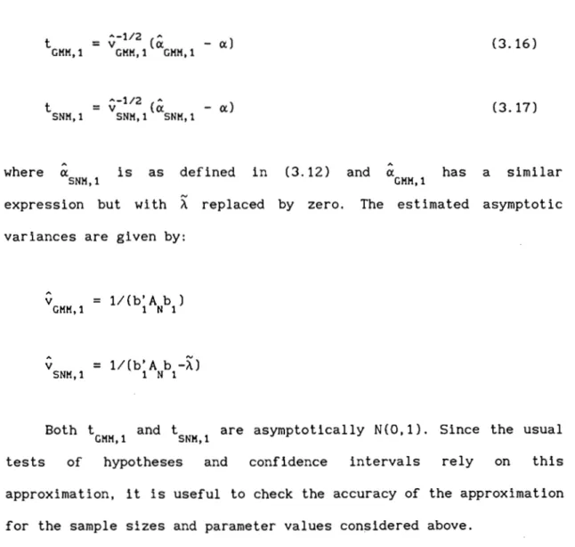
We have also investigated the flnite sample dlstributions of the standardized GMM and SNM "t-statistics" for Model 1 of the form

A-l/2 " t

₌

v (a - al (3.16) GMM,1 GMM,l GMH,I t SNH,l = "-1/2 .. v (a SNH,l SNH,l - a) (3.17) where is as defined in

-expression but with A replaced variances are given by:

(3.12) and by zero. The has estimated a similar asymptotic A V GHH,l

=

1I(b' A b )1 N 1 v

=

1/(b' A b -~l SNH,l 1 N 1

Both t and t a r e asymptotically N(O,l). Since the usual GMM,l SNK,1

tests of hypotheses and confldence intervals rely on thls approximation, lt is useful to check the accuracy of the approximatlon for the sample slzes and parameter values consldered aboye.

Table 5 reports finite sample quantlles of the t-statistics based on 10,000 replicatlons. We use a larger number of replications because

in this case the 0.9 and 0.95 quantiles in the upper tail of the distribution are of special interest. The median shows that the distributions of the GMM t-statistics are shifted to the left, w1th the absolute value of the shift increasing wi th ex, fT and T. In

1)

contrast, the distributions of the SNM t-statistics are centered at values very close to zero. Turning to the 0.9 and 0.95 quantiles, when T=4 the differences with the corresponding N(O.l) quantiles are always smaller for the SNM t-statistics than for the GMM, sometimes by a wide margino When T=7, the normal approximation worsens for both estimators. In that case, however, the upper-tail GMM quantiles tend to be closer to the normal values than those from the SNM t­ statistics.

4. Empirical Illustrations

Our first illustration of the previous methods proceeds by re­ estimating the employment equations presented by Arellano and Bond

(1991) using symmetrically normalized and indirect GMM estimators. The Arellano-Bond dataset consists on an unbalanced panel of 140 quoted companies from the UK, whose main activity 1s manufacturing and for which seven, eight or nine continuous annual observations are available for the period 1976-1984.

The models are all log-linear relationships between the number of employees, the average real wage, the stock of capital, a measure of industry output, lagged values of the previous variables, time dummies and company effects. The reader 1s referredto the Arellano and Bond article for a detailed description of the models and the data.

different models estimated in flrst differences using instrumental variables. Model A includes contemporaneous wage and capital variables, which are treated as endogenous along with the first lag of employment. In this model lagged sales and stocks are used as outside instruments in addition to lags of the endogenous variables included in the equation. Model B only includes lagged values of wages and capital and it could be interpreted as an approximated Euler equation for employment wi th quadratic adJustment costs. Columns labeled GMM reproduce some of the resul ts obtained by Arellano and Bond. The SNM estimates are calculated as described in Section 2, and for Model A there is an additional column containing indirect GMM estimates that were obtained by normalizing to unity the coefficient of contemporaneous wages. Fl na lly • the third panel of Table 6 presents GMM and SNM estimates of some simple second-order autoregressive models for employment with and without the inclusion of lagged wages.

As Table 6 shows, SNM and indirect GMM estimates are far apart from the direct GMM estimates. These results uncover the fact that the GMM estima tes from the dataset of UK flrms are probably much less reliable than what their estimated asymptotic standard errors would suggest. Interestingly, the SNM estimates of Model B are more compatible with the Euler equation interpretation than the GMM estima tes. For example, in the Euler equation discussed by Arellano and Bond the coefficient on n is given by (2+r) where r is the real

t-l

discount rateo

Our second empirical illustration is based on a similar but larger balanced panel of 738 Spanish manufacturing companies, for which there are available annual observations for the period 1983-1990

(see the AppendIx for a descrIption of these data). We cónsIder a bIvarIate V!\R model for the logarithms of employment and wages. The employment equation contalns both lagged employment and lagged wages, whIle the wage equatIon only Includes its own lags. ThIs model can be regarded as the reduced form of an intertemporal model of employment determInation under rational expectations (see Sargent (978». To obtain the reduced form, an !\R(2) process for log wages is assumed, and the Euler equation in the log of employment for the optimum contlngency plans is solved.

Table 7 presents GMM and SNM estimates of the two equations, flrstly using only lagged variables in levels as instruments for equations in flrst-differences (the baslc set of moment conditions that we called "Model 1"), and secondly adding lagged variables in first-differences as instruments for equations in levels (that is, including the stationarity restrictions of "Model 3"). For Model 1 we also report estimates of a univariate !\R(2) process for employment.

In addition to asymptotic confidence intervals, we calculated 95 percent semiparametric bootstrap confidence intervals based on 1000 replications from the empirical distribution function of the data subject to the moment restrictions (cf. Back and Brown (1993». Following Brown and Newey (1992) we drew the bootstrap samples from the mass-point distribution that estimated the probability of the i-th observation as

p

=

1/(1+l'W(y ,9»N

1 1

where

i

... 1 N '" 2

t

= argmin -N L 10g[t+t'ljJ(y,S)]

1=1 1

and ljJ(Yt'S) is the vector of orthogonality conditions for observation evaluated at the appropriate parameter estimates.

rabIe 7 contains some interesting results. GMM and SNM estimates of Model 1 are still different from each other but by a smaller margin than the corresponding estima tes for the UK panel. The difference becomes even smaller for the univarlate employment estlmates that are based on half the number of moments used for the estima tes in the first two columns. On the other hand, the estimates of Model 3 appear to be more precise, presumably because the additional orthogonality conditions are highly informative. In this case, GMM and SNM estimates provide very similar results. However, the Sargan statistics indicate a clear reJection of the stationarity restrictions in both the employment and the wage equations. It is also noticeable that although bootstrap confidence intervals are always larger than the asymptotic confldence intervals, the differences between the two are generally small.

\ole re-estimated Model 1 with a random subsample of 200 firms. which is similar to the size of the UK sample. Interestingly. the results (reported in rabIe 8) are closer to the UK results for similar specifications than those based on the full Spanish sample. In particular, the SNM estimates of the AR(2) model for employment are remarkably stable over the three datasets whlle standard GMM estima tes would be seriously downward biased in the smaller samples. Moreover, the discrepancies between asymptotic and bootstrap confidence

intervals in the random subsample were greater than in the full sample. 11

Finally, we simulated data as clase as possible to the AR(2) employment equation, to see if the findings that we obtained with the subsample of 200 companies were substantiated in the Monte CarIo simulations. Random errors and individual effects were generated from independent normal distributions with variances equal to the values estimated from the SNM residuals of the full Spanish sample. Since the estimated time effects showed very little variability, the constant was set to a common value for all periods gi ven by the average estimated time effect in levels, although the estimates in the simulations included time dummies. As a consequence the model was stationary, and we generated (and discarded) 100 preliminary observations for each individual to minimize the impact of ini tial conditions. The results are reported in Table 9, and confirm the impression conveyed by the real data. The SNM estimates are almost median unbiased, but GMM shows large downward biases, specially when N=200. A comparison in terms of median absolute errors also favours SNM for both sample sizes and parameter estimates. Lastly, looking at the quantiles of the t-ratios shown in the lower panel of Table 9, it appears that the N(O,l) approximation is reasonable for the SNM t­ ratios but not for the GMM t-ratios.

5. Conclusions

It has long been established that the lack of finite sample bias is an important advantage of LIML estimators of structural equations over 2SLS, which by contrast have thinner tails than LIML. The bias of 2SLS towards OLS can be specially worrying when the instruments are "poor" and/or the degree of overidentification is l~rge. In practice, this means that while LIML is invariant to normalization, often a 2SLS regression of y on x provides results that are fairly different from those of the (inverted) 2SLS regression of x on y, despite being asymptotically equivalent estimators. However, LIML has not been used much in applications. The reasons for this include a computational disadvantage over 2SLS, concerns with outliers, the fact that 2SLS can be more easily accommodated into the GMM framework, and we suspect that sometimes the use of an implicit prior that favored closeness to OLS when structural coefficients were poorly identified.

There has recently been a renewed interest in the finite sample properties of GMM estimators in various time series and cross­ sectional contexts. Several papers have emphasized the role of estimated weighting matrices for the properties of the estimators in small samples, and a number of alternative methods have been considered (eg. Altonji and Segal (1994), Hansen, Heaton and Varon (1995), Angrist, Imbens and Krueger (1995) or Imbens (1995). In contrast, in this paper we have focused on the role of normalization rules for the finite sample properties of GMM estimators that make use of standard two-step weighting matrices. Our work is motivated by the results in Hillier (1990), who argued that the alternative normalization rules adopted by LIML and 2SLS are at the basis of their

d1fferent sampling behaviour. Hillier showed that a symmetr1cally normal1zed 2SLS has similar finite sample propert1es to those of LIML. Th1s resul t 1s interestlng because, unlike LIML, SN-2SLS 1s a GMM est1mator based on structural form moment cond1t1ons and therefore 1t can be easlly extended to distr1butlon free env1ronments and robust statlstics.

In particular, SN-2SLS 1s well sulted for appl1catlon to the nonstandard IV s1tuations that arise in panel data models with predetermined variables, which are the models of interest in this papero These models are typically est1mated in first-differences using all the avallable lags as instruments. Usual1y, there is a large number of instruments avallable, but of poor quality since they tend to be only weakly correlated wl th the first-differenced endogenous variables that appear in the equation.

In this paper we have presented SN-GMM estimators for dynamic panel data models that are asymptotically equivalent to ordinary optimal GMM estimators. We have also showed how a byproduct of the estimation is a test statistic of overidentifying restrictions, based on a minimum eigenvalue calculatlon.

We have reported Monte CarIo evidence on the performance of GMM and SN-GMM est1mates for a flrst-order autoregress1ve model with individual effects. For this model we have considered three alternative sets of moment conditions as discussed by Arellano and Bond (1991), Ahn and Schmldt (1995), and Arellano and Bover (1995). Since for these models, the IV restr1ct1qns can be expressed as stralghtforward structures on the data covariance matrlx, using these representations we have also calculated MD and QML estimates for

comparisons with the IV estimates. Our findings suggest that Hillier's basic results may have a wider applicability. In most cases, SN-GMM is the estimator wi th the smallest median bias, and the one wi th the largest interquartile range. However, the differences in dispersion with ordinary GMM are small except in the almost unidentified cases.

Finally, as an empirical illustration, we havereported estima tes of employment and wage equations from UK and Spanish firm panels. The results show that GMM estimates from the (smaller) UK panel can be very unreliable when the degree of overidentification is large. The resul ts from the (larger) Spanish panel produce a closer agreement between ordinary and symmetrically normalized GMM estimates, although there is evidence that there can still be serious biases in GMM estimates. Some of these results are confirmed by simulating data as close as possible to the empirical data. Moment restricted bootstrap confidence intervals show that asymptotic confidence intervals are often over-optimistic, and Sargan tests consistently reject the restrictions implied by the stationarity of initial conditions.

Footnotes

1. Split sample or jackknife IV estlmators, however, arealso conslstent when the number of lnstruments tends to lnflnity (cL Angrlst and Krueger (1995) and Angrlst, Imbens and Krueger (1995»). 2. Empirical likellhood estlmators of the type considered by Qin and Lawless (1994) and Imbens (1995) w111 also be lnvariant to normalization due to the invariance property of ML estimators.

3. Notlce that i f the only explanatory exogenous variable in the equation is a constant term,

o

coincides wi th the orthogonal

SNM

regression on the fitted values Y (cf. Malinvaud (1970) and Anderson (1976»).

.... . . . . " 1/2

4. Meaning that the density of o: = b/(b' b) deflned on the unit circle is symmetric about the true points ±o:=±b/(b'b)1/2 having modes at ±o:.

5. This problem does not arise in the autoregressive panel data models discussed below, since in that case the SN-GMM estimator is invariant to units and to normalization.

6. I f no columns of X· are perfectly predictable from Z, or i f the entire vector of coefficients is normalized to unity, then Á = I and

A=min eigen(W·'M·W·), with W· = (y. ,X·).

7. However, they are not the only restrictions available since (3.2) also impl1es that nonlinear functlons of y~-2 are uncorrelated with

ÁV . The semiparametric efficiency bound for this model can be

l t

obtalned from the results in Chamberlain (1992). One reason why estimators based on (3.3) may not be fully efficient asymptotically is that the dependence between ~ and y T may be nonlinear. Another reason

i i

would be unaccounted conditional heteroskedasticity.

8. Notice that the (T-2) restrictions in (3.10) can also be written as (t=3, ... ,T)

For example, we have the identity

where u =y -o:y

9. In all cases, optlmlzatlon wlth respect to o: was conducted over the range

10:1

<1. Thls was achleved uslng the reparameterlzatlon

0:=2P/{1+p2) .

10. Means and standard devlations are not reported slnce the symmetrlcally normalized estimators, in common with

LIML.

can be expected to have lnfinite moments.

11. Bootstrap standard errors for the UK unbalanced panel were not calculated, since they would depend on a nontrivial specification of the empirical distribution function for the unbalanced observations.

References

Ahn, S. and P. Schmidt (1995), "Efficient Estimation of Models for Dynamic Panel Data, Journal of Econometrics, 68, 5-27.

Altonji, J. and L. Segal (1994), "Small-Sample Bias in GMM Estimation of Covariance Structures", NBER Technical Working Paper 156.

Anderson, T.W. (1976), "Estimation of Linear Functional Relationships: Approximate Distributions and Connections with Simultaneous Equations in Econometrics", Journal of the Royal Statistical Society, Series B, 38, 1-20.

Anderson, T.W., N. Kunitomo and T. Sawa (1982), "Evaluation of the Distribution Function of the Limited Information Maximum Likelihood Estimator", Econometrica, 50, 4, 1009-1027.

Angrist, J.D. and A.B. Krueger (1995), "Split Sample Instrumental Variables Estimates of the Return to Schooling", Journal of

Business and Economic Statistics, 13, 225-235.

Angrist, J. D. , G. W. Imbens and A. Krueger (1995) , "Jackknife Instrumental Variables Estimation", NBER Technical Working Paper 172.

Arellano, M. and S.R. Bond (1991), "Some Tests of Specification for Panel Data: Monte CarIo Evidence and an Application to Employment Equations, Review of Economic Studies, 58, 277-297.

Arellano, M. and O. Bover (1995), "Another Look at the Instrumental­ Variable Estimation of Error-Components Models" , Journal of

Econometrics, 68, 29-51.

Back, K. and D.P. Brown (1993), "Implied Probabilities in GMM Estimators", Econometrica, 61, 971-975.

Bekker, P.A. (1994), "Alternative Approximations to the Distributions of Instrumental Variable Estimators", Econometrica, 62, 657-681.

Bound, J., D.A. Jaeger and R. Baker (1995), "The Cure Can Be Worse than the Disease: A Cautionary Tale Regarding Instrumental Variables",

Journal of the American Statistical Association, April. Brown, B.W. and W.K. Newey (1992), "Bootstrapping for GMM", mimeo.

Chamberlain, G. (1982), "Multivariate Regression Models for Panel Data",

Journal of Econometrics, 18, 5-46.

Chamberlain, G. (1992), "Comment: Sequential Moment Restrictions in Panel Data", Journal of Business

&

Economic Statistics, 10, 20-26. Goldberger, A.S. and 1. Olkin (1971), "A Minimum-Distance Interpretation

of LImIted-Informatlon EstImatIon", Econometrlca, 39, 635-639. Hansen, L.P. (1982). "Large Sample Propertles of Generallzed Method of

Moments Estlmators", Econometrlca, 50, 1029-1054.

Hansen, L.P., J. Heaton and A. Varon (1995), "FInite Sample Propertles of Some Alternatlve GMM Estlmators", mImeo, Department of Economlcs, UnIversity of ChIcago.

Hilller. G.H. (1990), "On the Normallzatlon of Structural Equatlons: Propertles of Direction Estimators", Econometrlca, 58, 1181-1194. Holtz-Eakln, D., W. Newey and H. Rosen (1988), "EstlmatIng Vector

Autoregressions with Panel Data, Econometrlca, 56, 1371-1395.

Imbens, G. (1995), "One-step Estimators for Over-identlf1ed Generallzed Method of Moments Models". mimeo.

Keller, W. J. (1975), "A New Class of Limited-Information Estimators for Slmultaneous Equation Systems" , Journal of Econometrlcs, 3, 71-92. Kunitomo, N. (1980), "Asymptotlc ExpansIons of the Distributions of

Estimators in a Linear Functional Relationship and Simul taneous Equations", Journal of the American Statistical Association, 75,

693-700.

Malinvaud, E. (1970), Statistical Hethods of Econometrics, North­ Holland, Amsterdam.

Morimune, K. (1983), "Approximate Distributions of k-Class Estlmators when the Degree of OveridentifiabilIty Is Large Compared with the Sample Size", Econometrica, 51, 821-841.

Phillips, P.C.B. (1983), "Exact Small Sample Theory in the Simultaneous Equations Model" , in Griliches, Z. and M.D. lntriligator (eds.):

Handbook of Econometrics, vol. l, North-Holland, Amsterdam, Ch. 8.

Qin, J. and J. Lawless (1994), "EmpirIcal Likellhood and General Estimating Equations", Annals of Statistics, 22, 300-325.

Sargent, T.J. (1978), "Estlmatlon of Dynamic Labor Demand Schedules under Rational Expectations", Journal of Pol1t ical Economy, 86.

StaIger, D. and J.H. Stock (1994), "Instrumental Variables Regression with Weak Instruments", NBER TechnIcal Worklng Paper 151.

White, H. (1982), "Instrumental Variables Regression with Independent Observations", Econometrlca, 50, 483-499.