Testing for structural breaks
in dynamic factor models
Jörg Breitung
(University of Bonn and Deutsche Bundesbank)
Sandra Eickmeier
(Deutsche Bundesbank)
Discussion Paper
Editorial Board: Heinz Herrmann
Thilo Liebig
Karl-Heinz Tödter
Deutsche Bundesbank, Wilhelm-Epstein-Strasse 14, 60431 Frankfurt am Main, Postfach 10 06 02, 60006 Frankfurt am Main
Tel +49 69 9566-0
Telex within Germany 41227, telex from abroad 414431 Please address all orders in writing to: Deutsche Bundesbank,
Press and Public Relations Division, at the above address or via fax +49 69 9566-3077
Internet http://www.bundesbank.de
Reproduction permitted only if source is stated. ISBN 978-3–86558–500–4 (Printversion) ISBN 978-3–86558–501–1 (Internetversion)
Testing for structural breaks
in dynamic factor models
J¨
org Breitung
University of Bonn and
Deutsche Bundesbank
Sandra Eickmeier
∗Deutsche Bundesbank
Abstract
From time to time, economies undergo far-reaching structural changes. In this paper we investigate the consequences of structural breaks in the factor loadings for the specification and estimation of factor models based on principal components and suggest test procedures for structural breaks. It is shown that structural breaks severely in-flate the number of factors identified by the usual information criteria. Based on the strict factor model the hypothesis of a structural break is tested by using Likelihood-Ratio, Lagrange-Multiplier and Wald statistics. The LM test which is shown to perform best in our Monte Carlo simulations, is generalized to factor models where the common factors and idiosyncratic components are serially correlated. We also apply the suggested test procedure to a US dataset used in Stock and Watson (2005) and a euro-area dataset described in Altissimo et al. (2007). We find evidence that the beginning of the so-called Great Moderation in the US as well as the Maastricht treaty and the han-dover of monetary policy from the European national central banks to the ECB coincide with structural breaks in the factor loadings. Ignor-ing these breaks may yield misleadIgnor-ing results if the empirical analysis focuses on the interpretation of common factors or on the transmission of common shocks to the variables of interest.
∗The views expressed in this paper do not necessarily reflect the views of the Deutsche
Bundesbank. This paper was presented at the Workshop on Panel Methods and Open Economies, Frankfurt/Main, May 21, 2008 and at the International Conference on Factor Structures for Panel and Multivariate Time Series Data, Maastricht, September 19–20, 2009. The authors would like to thank Joern Tenhofen for many helpful comments and suggestions. Address: Joerg Breitung, University of Bonn, Institute of Econometrics, 53113 Bonn, Germany. Email: [email protected]
Keywords: Dynamic factor models, structural breaks, number of factors, Great Moderation, EMU
Non-technical summary
Analyzing data sets with a large number of variables and time periods involves a severe risk that some of the model parameters are subject to structural breaks. Dynamic factor models may be more affected by this issue than other econometrics models, since factor models rely on large datasets. In this paper we investigate the consequences of structural breaks in the factor loadings for the specification and estimation of factor models based on principal components and suggest test procedures for structural breaks. In our theoretical analysis, we first consider the effects of structural breaks. It turns out that structural breaks in the factor loadings increase the dimension of the factor space. The reason is that in the case of a single structural break, two sets of common factors are needed to represent the common components in the two subsamples before and after the break. Thus, structural breaks in the factor loadings do not only lead to inconsistent estimates of the loadings but also to a larger dimension of the factor space. If we are only interested in decomposing variables into common and idiosyncratic components, it is sufficient to increase the number of factors such that the factor space is large enough to represent the different subspaces of the two regimes. However, if we are interested in a more parsimonious factor representation that allows us to recover the original factors, the estimation has to account for the structural breaks in the factor loadings. It is therefore very important to have tests at hand which inform us about whether or not structural breaks exist.
Furthermore, we propose Chow type tests for structural breaks in factor models. It is shown that under the assumptions of an approximate factor model and if the number of variables is sufficiently large, the estimation error of the common factors does not affect the asymptotic distribution of the Chow statistics. In other words, the principal component estimator of the common factors is “super-consistent” with respect to the estimation of the factor loadings and, therefore, the usual Chow test can be applied to the factor model in a regression, where the unknown factors are replaced by principal components. Provided that the idiosyncratic components are mutually independent, i.e. under the assumption of a strict factor model, the
by adopting a GLS version of the test. This approach assumes a finite order autoregressive process for the idiosyncratic components, whereas no specific dynamic process needs to be specified for the common factors. Our Monte Carlo simulations suggest that the LM version outperforms the other variants of the test. The LM test procedure is applied to two different settings. Our first empirical application uses a large US macroeconomic dataset. We have tested whether the so called Great Moderation in the US (assuming the first quarter of 1984 as the starting date) coincides with structural breaks in the factor loadings. A lot of attention among researchers and policy makers has recently been directed to the Great Moderation. There is still some controversy about the sources (“good luck” versus structural changes including “good policy”), and we contribute to this debate. We find evidence of “dramatic changes” in the economy, reflected in significant breaks in the factor loadings, in the mid-1980s. By testing for breaks in the loadings of individual variables we can assess the underlying sources of the structural change. We find support for the hypothesis that not a single but various factors have played an important role. These factors are, according to our analysis, changes in the conduct of monetary policy, in inventory management as well as financial integration.
In the second application we employ a large euro-area dataset to test whether structural breaks have occurred in the euro area around two major events, the signing of the Maastricht treaty in the second quarter of 1992 and the creation of the ECB in the first quarter of 1999. This setting is particularly interesting, since these events may have altered comovements between variables, and this would just be reflected in structural breaks in the factor loadings. We find evidence of structural breaks around both dates. The null hypothesis of no structural break was rejected for more variables when the ECB was created than when the Maastricht treaty was signed. It is equally likely that breaks have occurred exactly in 1999 and just before the creation of the ECB which may have been anticipated or due to prior adjustments. Breaks finally seem to have occurred around the two events relatively
variables, whereas the signing of the Maastricht treaty seems to coincide with breaks in the factor loadings of industrial production series.
Nichttechnische Zusammenfassung
Die Analyse von Datensätzen mit einer Vielzahl an Variablen und Zeiträumen birgt das Risiko, dass einige der Modellparameter Strukturbrüchen unterworfen sind. Dynamische Faktormodelle können von diesem Problem stärker betroffen sein als andere ökonometrische Modelle, da Faktormodelle auf große Datensätze zurückgreifen.
Im vorliegenden Papier untersuchen wir schwerpunktmäßig theoretisch die Folgen von Strukturbrüchen in den „Faktorladungen“ (welche das Ausmaß angeben, in dem Faktoren die Variablen beeinflussen) für die Spezifizierung und Schätzung von Faktormodellen auf Basis von Hauptkomponenten und schlagen Verfahren für Tests auf Strukturbrüche vor. Anschließend wenden wir die formalen Tests auf zwei empirische Fragestellungen an: die so genannte „Great Moderation“ in den USA und den europäischen Integrationsprozess.
In unserer theoretischen Analyse betrachten wir zunächst die Auswirkungen von Strukturbrüchen. Es stellt sich heraus, dass Strukturbrüche in den Faktorladungen die Dimension des Faktorraums erweitern. Grund hierfür ist, dass im Falle eines einzelnen Strukturbruchs doppelt so viele gemeinsame Faktoren benötigt werden, um die gemeinsamen Komponenten in den beiden Teilstichproben vor und nach dem Bruch abzubilden. Somit führen Strukturbrüche in den Faktorladungen nicht nur zu inkonsistenten Schätzungen der Ladungen, sondern auch zu einer größeren Dimension des Faktorraums. Gilt unser Interesse nur der Zerlegung der Variablen in gemeinsame und in idiosynkratische (d.h. variablen-spezifische) Komponenten, so reicht es aus, die Zahl der Faktoren so weit zu erhöhen, dass der Faktorraum groß genug ist, um die verschiedenen Unterräume der beiden Regime darzustellen. Sind wir dagegen an einer einfacheren Faktordarstellung interessiert, die uns die Schätzung der Originalfaktoren ermöglicht, so sind in der Schätzung die Strukturbrüche in den Faktorladungen zu berücksichtigen. Daher ist es sehr wichtig, Tests zur Hand zu haben, die uns Auskunft darüber geben, ob ein Strukturbruch vorliegt oder nicht.
Dementsprechend schlagen wir Chow-Tests auf Strukturbrüche in Faktormodellen vor. Es wird gezeigt, dass der Schätzfehler der gemeinsamen Faktoren unter der Annahme eines approximativen Faktormodells und der Voraussetzung einer hinreichend großen Anzahl an Variablen die asymptotische Verteilung der Chow-Statistik nicht beeinflusst. Mit anderen Worten: Der Hauptkomponentenschätzer der gemeinsamen Faktoren ist „super-konsistent“ in Bezug auf die Schätzung der Faktorladungen, und daher kann der gewöhnliche Chow-Test in einer Regression, bei der die unbeobachteten Faktoren durch Hauptkomponenten ersetzt werden, auf das Faktormodell angewandt werden. Sofern die idiosynkratischen Komponenten gegenseitig unabhängig sind, d. h. unter der Annahme eines strikten Faktormodells, lassen sich die variablenspezifischen Chow-Statistiken zusammenfassen, um die gemeinsame Nullhypothese eines gemeinsamen Strukturbruchs zu testen. Diese Tests können durch den Einsatz einer GLS-Version des Tests verallgemeinert und auf dynamische Faktormodelle angewandt werden. Dieser Ansatz unterstellt für die idiosynkratischen Komponenten einen endlichen autoregressiven Prozess, während für die gemeinsamen Faktoren kein bestimmter dynamischer Prozess spezifiziert werden muss. Unsere Monte-Carlo-Simulationen sprechen dafür, dass die LM-Version den anderen Varianten des Tests überlegen ist.
Das LM-Testverfahren wird auf zwei unterschiedliche Fragestellungen angewandt. Bei unserer ersten empirischen Anwendung wird getestet, ob die sogenannte „Great Moderation“ in den Vereinigten Staaten, d.h. der Rückgang der Volatilität verschiedener makroökonomischer Größen, mit Strukturbrüchen in den Faktorladungen einhergeht. Das Phänomen der Great Moderation hat in der letzten Zeit große Aufmerksamkeit erfahren. Die Ursachen sind nach wie vor umstritten („Glück“ oder strukturelle Veränderungen einschließlich „guter Politik“). Wir tragen zu dieser Debatte bei und finden Belege für generelle „dramatische Veränderungen“ in der Volkswirtschaft, die in signifikanten Brüchen in den Faktorladungen Mitte der Achtzigerjahre zum Ausdruck kommen. Mit Hilfe von Tests auf Brüche in den Ladungen einzelner Variablen können wir die zugrunde liegenden Ursachen der strukturellen Veränderungen feststellen. Wir finden Belege für die Hypothese, dass nicht ein einzelner, sondern verschiedene Faktoren eine wichtige Rolle gespielt haben. Hierzu zählen unserer Analyse zufolge Änderungen in der Durchführung der
In der zweiten Anwendung ziehen wir einen umfangreichen Datensatz des Euro-Währungsgebiets heran, um zu testen, ob es im Euroraum zur Zeit zweier bedeutender Ereignisse - der Unterzeichnung des Maastricht-Vertrags im zweiten Quartal 1992 und der Gründung der EZB im ersten Quartal 1999 – zu Strukturbrüchen kam. Diese Fragestellung ist besonders interessant, weil diese Ereignisse den Gleichlauf zwischen Variablen verändert haben könnten, was sich gerade in Strukturbrüchen in den Faktorladungen widerspiegeln würde. Wir finden Belege für Strukturbrüche um beide Zeitpunkte herum. Es scheint, dass mehr Strukturbrüche zur Zeit der Gründung der EZB aufgetreten sind als zum Zeitpunkt bei Unterzeichnung des Maastricht-Vertrags. Es ist dabei in etwa gleich wahrscheinlich, dass die Brüche sich genau im Jahr 1999 oder kurz vor Gründung der EZB ereigneten. Möglicherweise wurden das Ereignis von Marktteilnehmern antizipiert und entsprechende Anpassungen vorweggenommen. Schließlich traten die Brüche um die beiden Ereignisse herum offenbar relativ häufig in den Ladungen der Variablen auf, die die Volkswirtschaften Spaniens und Italiens abbilden, in denen die Notwendigkeit der Konvergenz auch am größten war. Die Gründung der EZB ging mit relativ häufigen Strukturbrüchen in den Ladungen nominaler Variablen einher, während die Unterzeichnung des Maastricht-Vertrags zeitlich mit Brüchen in den Faktorladungen der Industrieproduktionsreihen zusammenzufallen scheint.
Contents
1 Introduction 1
2 The effect of structural breaks on the number of factors 3
3 The static factor model 5
4 Dynamic factor models 8
5 Empirical applications 12
5.1. The US economy in the mid-1980s 12
5.2. Have the Maastricht treaty and the creation of the ECB
led to structural breaks in the euro area? 17
6 Conclusions 21
Appendix 23
Tables and Figures
Table 1 Average of the estimated number of factors 35
Table 2 Empirical sizes 36
Table 3 Size adjusted power against a break at T* = T/2 36
Table 4 Empirical sizes in the dynamic model: Joints tests 37 Table 5 Empirical sizes in the dynamic model: Individual tests 38
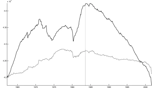
Table 6 Tests for structural break (US data) 39
Table 7 Tests for specific variables (US data) 39 Table 8 Tests for structural breaks (r = 9) 40
Table 9 Tests for specific variables 40
Figure 1 LM test statistic (US data) 41
Figure 2 Relative frequencies of rejections (US data) 42
Figure 3 Log likelihood (US data) 43
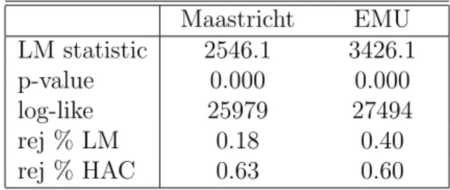
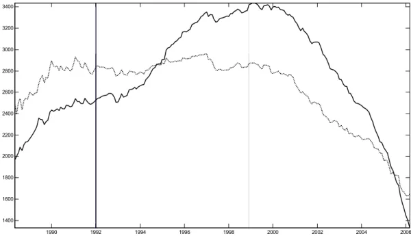
Figure 4 LM test statistic (EMU data) 44
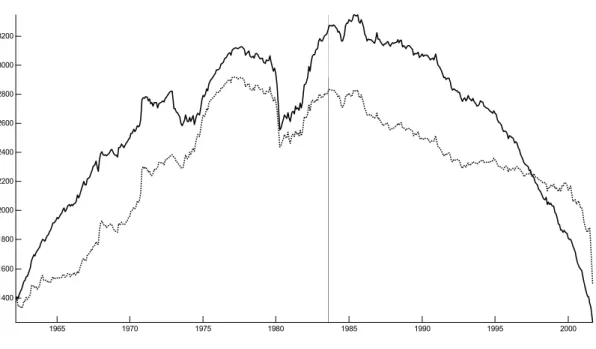
Figure 5 Relative frequencies of rejections (EMU data) 45
1
Introduction
In recent years dynamic factor models have become popular for analyzing and forecasting large macroeconomic datasets. These datasets include hun-dreds of variables and span large time periods. Thus, there is a substantial risk that the data generating process of a subset of variables or all variables have undergone structural breaks during the sampling period. Stock and Watson (2002) argue that factor models are able to cope with either breaks in the factor loadings in a fraction of the series, or can account for moderate parameter drift in all the series. However, in empirical applications param-eters may change dramatically due to important economic events, such as the collapse of the Bretton Woods system, or changes in the monetary policy regime, such as the conduct of monetary policy in the 1980s in the US or the formation of the European Monetary Union. There may also be more grad-ual but nevertheless fundamental changes in economic structures that may have led to significant changes in the comovements of variables, such as those related to globalization and technological progress. The common factors may become more (less) important for some of the variables and, therefore, the loading coefficients attached to the common factors are expected to become larger (smaller). If one is interested in estimating the common components or assessing the transmission of common shocks to specific variables, ignoring structural breaks may give misleading results.
Variations in dynamic factor loadings have been considered before. The study most closely related to ours is Stock and Watson (2007) who study the implications of structural breaks in the factor loadings. Consequently, we will compare our with their testing approach. Del Negro and Otrok (2008) have suggested a model where the factor loadings are modelled as random walks. This comes, however, at the cost of having to estimate many parameters which is computationally expensive and probably not feasible for such large datasets we will use in our empirical applications below. Finally, Banerjee and Marcellino (2008) have investigated the consequences of time-variation in the factor loadings for forecasting based on Monte Carlo simulations and find it to worsen the forecasts, in particular in small samples.
In our theoretical analysis, we first consider the effects of structural breaks in section 2. It turns out that structural breaks in the factor loadings
crease the dimension of the factor space. The reason is that in the case of a single structural break, two sets of common factors are needed to represent the common components in the two subsamples before and after the break. Thus, structural breaks in the factor loadings do not only lead to inconsistent estimates of the loadings but also to a larger dimension of the factor space. If we are only interested in decomposing variables into common and idiosyn-cratic components, it is sufficient to increase the number of factors such that the factor space is large enough to represent the different subspaces of the two regimes. However, if we are interested in a more parsimonious factor representation that allows us to recover the original factors, the estimation has to account for the structural breaks in the factor loadings.
In section 3, we consider alternative versions of a Chow-type test for a structural break in a strict factor model, where the components are assumed to be white noise. The idea is to treat the estimated factors as if they were known. We show that under certain conditions on the relative rate of N and T the estimation error of the common factors does not affect the asymptotic distribution of the test statistic. Our Monte Carlo experiment suggests that although the three versions of the test (Lagrange-Multiplier (LM), Likelihood-Ratio (LR), and Wald (W)) are asymptotically equivalent, these tests may perform quite differently in small samples, where the LM statistic has the best size properties.
In section 4, the LM test procedure is generalized to allow for serially correlated factors and idiosyncratic components. By adapting the GLS es-timation procedure suggested by Breitung and Tenhofen (2008) we obtain a test procedure that is robust to individual-specific dynamics of the compo-nents. The LM version of the test is shown to have reliable size properties whereas the OLS based test statistic with robust standard errors used in Stock and Watson (2007) performs rather poorly in finite samples.
Two empirical applications of the test procedures are presented in sec-tion 5. Based on a large US macroeconomic dataset provided by Stock and Watson (2005), we examine whether January 1984 (which is usually associ-ated with the beginning of the so called Great Moderation) coincides with a structural break in the factor loadings. Based on the LM test, we find clear evidence of a break at that date. By testing for shifts in the loadings
of individual variables we are able to shed light on the sources of the break. We also apply the LM test to a large euro-area dataset used in Altissimo et al. (2007). We find evidence for breaks at the dates of the Maastricht treaty and the creation of the European Central Bank (ECB). Breaks seem to have occurred relatively frequently in the loadings of variables capturing the Spanish and the Italian economies. The creation of the ECB was asso-ciated with relatively frequent structural breaks in the loadings of nominal variables, whereas evidence of structural breaks is mainly found for industrial production series around the signing of the Maastricht treaty.
2
The effect of structural breaks on the
num-ber of factors
Consider a factor model with r factors1 ft = [f1t, . . . , frt] that is subject to a common break at time T∗:
yit = ftλ(1)i +εit for t= 1, . . . , T∗ (1)
yit = ftλ(2)i +εit for t=T∗+ 1, . . . , T, (2)
where t = 1, . . . , T denotes the time period and i = 1, . . . , N indicates the cross-section unit. The assumption of a common structural break at T∗ is made for convenience only. A generalization to situations with variable-specific break dates is straightforward but implies an additional notational burden. The vector of idiosyncratic errors ε·t = [ε1t, . . . , εNt] is assumed to be i.i.d. with covariance matrixE(ε·tε·t) = Σ, where Σ is a diagonal matrix. Furthermoreftis assumed to be white noise with positive definite covariance matrix E(ftft) = Φ. Let Λ(k) = [λ(k)
1 , . . . , λ(Nk)], k = 1,2, and τ = T∗/T ∈
(0,1) denotes the relative break date. The unconditional covariance matrix of the vectory·t = [y1t, . . . , yNt] results as
E 1 T T t=1 y·ty·t = τΛ(1)ΦΛ(1)+ (1−τ)Λ(2)ΦΛ(2) + Σ ≡ Ψ + Σ.
1Note that the notation does not refer to a particular normalization of the (true) common factors. In our asymptotic considerations we follow Bai (2003) and adopt a particular normalization such thatT−1Tt=1ftft →p Ir.
Since the matrix Ψ =τΛ(1)ΦΛ(1)+ (1−τ)Λ(2)ΦΛ(2) is a sum of two matrices of rank r, the rank of the covariance matrix of the common component, Ψ, is 2r in general. This is due to the fact that a break in the factor loadings implies two linearly independent factors for the first and second subsample. It follows that if the structural break in the factor loadings is ignored the number of common factors is inflated by a factor of two. More generally, if there arek structural breaks in the factor loadings of r common factors, the number of factors for the whole sample is (k+ 1)r, in general.
The practical implication of this result is that if one is only interested in a decomposition of the time series yit into a common component and an idiosyncratic component, then it is sufficient to increase the number of common factors accordingly. However, if one is interested in a consistent estimator of the factors and the factor loadings, then it is important to account for the break of the factor loadings, e.g. by splitting the sample atT∗ and re-estimating the factor model for the two subsamples. For illustration consider the previous example with r = 1, T∗ = T/2 and λ(2)i = λ(1)i +b. Define an additional factor as
f∗
t =
ft for t = 1, . . . , T∗
−ft for t =T∗+ 1, . . . , T.
It is not difficult to see that the factor model with a structural break can be represented as
yit =λ∗1ift+λ∗2ift∗+εit (3)
where λ∗1i = λ(1)i + (b/2) and λ∗2i = −b/2. Note that the factors in this representation are “orthogonal” in the sense that E(T−1Tt=1ftft∗) = 0. This example demonstrates that a factor model with structural break admits a factor representation with a higher dimensional factor space.
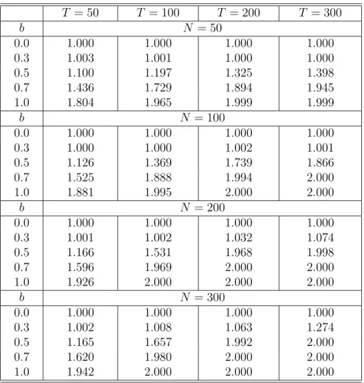
To investigate the effects of a structural break on the information criteria suggested by Bai and Ng (2002) for selecting the number of common factors a Monte Carlo experiment is performed. The data is generated by a factor modelyit =λitft+εit, where the single factorftand idiosyncratic components are i.i.d. with variances E(ft2) = 1 and E(ε2it) =σi2, where σi ∼ U(0.5,1.5). The structural break in the loadings is specified as
λit =
λi for t= 1, . . . , T/2
and λi is drawn from a N(1,1) distribution. Therefore, the parameter b measures the importance of the structural break. Table 1 presents the average of the number of factors selected by the ICp1 criterion suggested by Bai and Ng (2002). The results show that if the break is large, the selection procedure overestimates the number of common factors. Our theoretical reasoning suggests that the empirical procedure tends to identify two factors instead of the single factor that is used to generate the data. Thus, ignoring a break in the factor loadings tends to identify too many factors in the sample. This may be misleading and a result of structural breaks.
It is interesting to note that the situation is comparable to the problem of estimating a dynamic factor model within a static framework. As argued by Stock and Watson (2002), lags of the original factors can be accounted for by including additional factors. If one is merely interested in a decom-position into common and idiosyncratic components (e.g. in forecasting), then it is sufficient to estimate the static representation with a larger num-ber of factors. However, if one is interested in the original (“primitive” or “dynamic”2) factors, then the static factors are inappropriate as they involve linear combinations of current and lagged values of the original factors.
3
The static factor model
Consider a model with a common structural break at period T∗ as given in (1) and (2). Under the null hypothesis we assume
H0 : λ(1)i =λ(2)i . (4)
To test this null hypothesis, the usual Chow test statistics are formed by replacing the unknown vector of common factors,ft, by its principal compo-nents (PC) estimator, ft. Applying the likelihood ratio principle for testing the i’th variable gives rise to the statistic
lri =T
log(S0i)−log(S1i+S2i) ,
where S0i = T t=1 (yit−ftλi)2 S1i = T∗ t=1 yit−ftλ(1)i 2 S2i = T t=T∗+1 yit−ftλ (2) i 2 ,
λi denotes the PC estimator for the vector of factor loadings, whereas λ(1)i
and λ(2)i denote the two estimates obtained as the OLS estimates from a regression of yit on ft for two subsamples according to t = 1, . . . , T∗ and
t=T∗+ 1, . . . , T.3
The second statistic is the Wald test of the hypothesis ψi = 0 in the regression yit=λift+ψift∗+vit, t= 1, . . . , T, (5) where f∗ t = 0 fort = 1, . . . , T∗ ft fort =T∗+ 1, . . . , T. (6)
The resulting test statistic is denoted by wi.
The LM (score) statistic, indicated by si is obtained from running a re-gression of the form
εit =θift+φift∗+eit , (7)
where εit = yit−λift denotes the estimated idiosyncratic component. The score statistic is denoted by si =T R2i, where R2i denotes the R2 of the i’th regression.
To study the limiting null distributions of the three test statistics we first invoke the usual assumptions of the approximate factor model.
3Alternatively, the subsample estimates may be obtained from two separate PC estima-tions. The resulting test is asymptotically equivalent to the version suggested here, since the asymptotic properties of the regression are not affected by the estimation error offt. However, the analysis of the former estimator is complicated by the fact that not only the estimated loadings are different under the null and alternative hypothesis but also the estimated factors. We therefore focus on the simpler regression version which performs very similar to the test based on two separate PC estimations.
Assumption 1: Letyitbe generated by the factor modelyit=λift+εit, where it is assumed that λi, ft, and εit satisfy Assumptions A–G of Bai (2003).
This set of assumptions allows for some weak serial and cross-section depen-dence and heteroskedasticity among the idiosyncratic components εit. Fur-thermore, the factors and idiosyncratic components are allowed to be weakly correlated such that
E ⎛ ⎝1 N N i=1 1 √ T T t=1 ftεit 2⎞ ⎠<∞.
Under assumption 1 and√T /N →0 the estimation error in the regressorft does not affect the asymptotic distribution of the test statistic. To establish the usual asymptoticχ2 distribution of the Chow test, a more restrictive set of assumptions is required:
Assumption 2: (i) For all t = 1, . . . , T, E(ε2it) = σ2i and E(εitεis) = 0 for
t=s. (ii) ft is independent of εis for all i, t, s.
The null distributions of the test statistics are presented in the following theorem.
Theorem 1: Under Assumptions 1 and 2, T → ∞, N → ∞, and√T /N →
0, the statistics si, wi and lri have a χ2 limiting distribution with r degrees of freedom.
Remark A:The individual tests can be combined by constructing thepooled test statistics LR∗ = N i=1lri −rN √ 2rN , W ∗ = N i=1wi −rN √ 2rN , LM ∗ = N i=1si −rN √ 2rN , which are the standardized versions of the average test statistics. The correc-tions are due to the fact that the χ2 distribution with r degrees of freedom has expectation r and variance 2r. Under the additional assumption that
εit and εjt are independent for all i = j, the pooled test statistics have a
standard normal limiting distribution.
Remark B: It is important to select the appropriate number of common factors as otherwise the test may lack power. If the number of common
factors is determined from the entire sample, the identification criteria tend to select a larger number of common factors. As has been argued in section 2, a factor model with a structural break admits a (parameter constant) factor representation with a larger number of factors. Therefore, the number of factors should be selected by applying the information criteria of Bai and Ng (2002) to the subsamples before and after the break.4
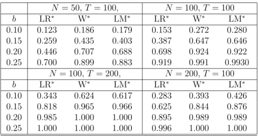
To investigate the finite sample properties of the test statistics, a Monte Carlo experiment is performed. We simulate data according to the single factor modelyit =λ(ik)ft+εit, where the factor and idiosyncratic components are generated as in section 2. The empirical sizes of the three different test statistics LR∗, W∗, and LM∗ are presented for various sample sizes in Table 2. It turns out that for all N and T the actual size of the LM statistic is close to the nominal size of 0.05. On the other hand, the LR statistic shows a tendency to reject the null hypothesis slightly too often, whereas the size bias of the Wald test tends to increase with fixed T and N → ∞.
Table 3 presents the empirical power of the test statistics forT ∈ {100,200} and N ∈ {50,100,200}. The structural break is again modeled as a shift of sizebin the mean of the factor loadings (see section 2). Note that the LR and Wald statistics have a moderate size bias that is accounted for by presenting the size-adjusted power. It turns out that the LM and Wald statistics are substantially more powerful than the LR statistic, whereas the former two test statistics perform very similar. Since our simulation experiment (based also on models with more factors and other data generating mechanisms) clearly favors the LM tests, we focus on this test statistic in what follows.
4
Dynamic factor models
In the previous section we have considered the framework of a static factor model, where the common and idiosyncratic components are white noise. In many practical situations, however, the variables are generated by dynamic processes. In this section we therefore generalize the factor model and assume that the idiosyncratic components in the modelyit =λift+uit are generated
4We are grateful to Peter Boswijk who has pointed out this problem during the con-ference.
by individual specific AR(pi) processes
uit = i,1ui,t−1+· · ·+i,piui,t−pi+εit (8)
i(L)uit = εit, (9)
wherei(L) = 1−i,1L− · · · −i,piLpi. To analyze the asymptotic properties
of the tests in a dynamic factor model we make the following assumption.
Assumption 3: (i) The idiosyncratic components are generated by (9), where all roots of the autoregressive polynomial i(z) are outside the unit circle. (ii) For all t E(ε2it) = σ2i and E(εitεis) = 0 for t = s. (iii) ft is independent of εis for all i, t, s.
The dynamic process for the vector of common factors is left unspecified. We only assume that the second moments are finite, i.e., the limitT−1Tt=1ftft →p Σf is a finite positive definite matrix (see Assumption A in Bai (2003)).
To test for structural breaks, Stock and Watson (2007) suggest to apply conventional Chow tests for each variable yit, where the unobserved factors are replaced by estimates obtained from applying principal components. A possible serial correlation of the errors is accounted for by using heteroskedas-ticity and autocorrelation consistent (HAC) estimators for the standard er-rors of the coefficients (cf. Newey and West 1987). This approach has, however, two important drawbacks. First, since the OLS estimator is ineffi-cient in the presence of autocorrelated errors, the resulting test suffers from a loss of power relative to a test based on a GLS estimator. Second, it is well known that the HAC estimator may perform poorly in small samples. This problem may be amplified when forming a joint test for all variables, since the joint test results from the sum ofN test statistics. Indeed, this is what we observe in our Monte Carlo simulation presented below.
To sidestep these difficulties, we follow Breitung and Tenhofen (2008) and compute the test statistic based on a GLS estimation of the model. The GLS transformed model results as
i(L)yit=λi[i(L)ft] +ψi[i(L)ft∗] +νit, (10)
where ft denotes the PC estimator of the common factors, ft∗ = ft for t =
T∗+ 1, . . . , T andf∗
can be estimated by running least squares regressions
uit=i,1ui,t−1+· · ·+i,piui,t−pi+eit , (11)
whereuit is the PC estimator of the idiosyncratic component. The lag length
pi can be determined by employing the usual information criteria. To test
the hypothesis of no structural break at T∗, the LM statistic for ψi = 0 is computed. The resulting test statistic is denoted bysi. We focus on the LM statistic as this statistic possesses the best size properties among all tests considered in section 3. The following theorem states that the asymptotic null distribution of the resulting LM test statistic is the same as in Theorem 1.
Theorem 2: Let si denote the LM statistic for ψi = 0 in the regression
i(L)yit=λi[i(L)ft] +ψi[i(L)ft∗] +νit, t=pi+ 1, . . . , T. (12)
Under Assumptions 1 and 3, T → ∞, N → ∞, and √T /N → 0, si is asymptotically χ2 distributed with r degrees of freedom.
Remark C: Assumption 3 rules out temporal heteroskedasticity of the id-iosyncratic components. It is well known that the Chow test is not robust against a break in the variances. To obtain a robust statistic in the case of serial heteroskedasticity, the approach of White (1980) can be adopted. Al-ternatively, a GLS variant of the test statistic that is robust against a break in the variance atT∗ can be constructed as
for t= 1, . . . , T∗ : 1 σ(1)i i(L)yit =λ i 1 σi(1)i(L)ft +ψi 1 σ(1)i i(L)f ∗ t +νit for t=T∗+ 1, . . . , T : 1 σ(2)i i(L)yit =λ i 1 σi(2)i(L)ft +ψi 1 σ(2)i i(L)f ∗ t +νit.
Remark D: As in Remark A the variable-specific test statistics can be combined to obtain the pooled test statistics:
LM∗ = N i=1si −rN √ 2rN
Under similar assumptions as in Remark A, the test statistics have a standard normal limiting distribution.
To investigate the small sample properties of the test, we generate the factor as ft = 0.8ft−1+νt.5 The idiosyncratic errors are generated by the model
uit =ui,t−1+εit
for all i = 1, . . . , N. For the variances we set E(νt2) = 1 and E(ε2it) = σ2i, where σi ∼ U(0.5,1.5). The factor loadings are obtained from independent draws of aN(1,1) distribution. Table 4 presents the empirical sizes for the joint LM test and Table 5 reports the mean rejection rates for the individual tests si. The tests assume that the break occurs at period T∗ =T/2.
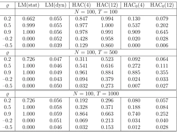
To assess the size bias that results from ignoring the serial correlation of the idiosyncratic component we first present the ordinary LM statistic that assumes white noise errors. As can be seen from the first column of Table 4, the rejection rates of the test are far from the nominal size of 0.05 even if the autoregressive coefficient is fairly small. In contrast, the actual size of the LM statistic computed from the GLS regression is close to the nominal size for all values of . The columns labelled as HAC(k) report the actual sizes of the OLS-based t-statistics employing robust standard errors, where the truncation lag is specified by applying the rule
T(k) =k(T/100)2/5 withk ∈ {4,12}. (13)
Since we found that the sizes are more reliable if the test is computed us-ing the LM principle, we also compute the HAC standard errors from the residuals of the restricted regression (i.e. where we have imposed the null hypothesis). The resulting test statistics are indicated by HAC0(k).
5Since the data generating process for f
t is irrelevant for the asymptotic properties of
From the results presented in Table 4 it turns out that the test statistics based on HAC standard errors perform very poorly in small samples. The test based on the restricted residuals (HAC0(k)) performs much better but still has a considerable size bias. To demonstrate that the size bias of these tests is indeed a small sample phenomenon, we repeat the simulations for
T = 500 and T = 1000. The results show that if T increases, the empirical sizes of the original HAC(k) slowly tend to the nominal size. Comparing the results for the joint test (Table 4) and the individual tests (Table 5) it turns out that the individual tests are more robust to small sample distortions than the joint tests. Additional simulation experiments suggest that the distortions become even more severe if the break date moves towards the beginning or end of the sample.
5
Empirical applications
Our test procedure is applied to two settings. In subsection 5.1, we investigate whether the mid-1980s in the US can be associated with structural breaks in the loadings. In subsection 5.2., we consider possible breaks in the euro-area economies due to the two major events in the 1990s, the Maastricht treaty and the creation of the ECB.
5.1
The US economy in the mid-1980s
In this section we apply our test procedure to the dataset constructed by Stock and Watson (2005) and provided on Mark Watson’s web page. The dataset contains 132 monthly US series including measures of real economic activity, prices, interest rates, money and credit aggregates, stock prices, and exchange rates. It spans 1960 to 2003.6 We investigate whether the mid-1980s in the US can be associated with structural breaks in the factor loadings. We also address important issues that typically arise in applications.
We start by considering a single break in 1984:01. That date has been associated with the beginning of the so called Great Moderation, i.e. the de-cline in the volatility of output growth and inflation (Kim and Nelson 1999,
6The original dataset is provided for the period 1959 to 2003. Some observations are, however, missing in 1959. We therefore decided to use a balanced dataset starting in 1960.
McConnell and Perez-Quiros 2000, Stock and Watson 2007). The focus on the 1984:01-break date and the use of the dataset is mainly motivated by the empirical application presented in Stock and Watson (2007) to which we can compare our results. Stock and Watson (2007) also test for structural breaks in the factor loadings in 1984:01 and use a very similar dataset. The main difference is that their dataset is quarterly and also covers more recent years (up to 2006). Another motivation of our application is that the sources of the Great Moderation are still controversial. Previous papers have applied structural break tests to univariate linear and univariate Markov-Switching models or, more recently, structural VAR models with time-varying param-eters to tackle this question. They have come up with various explanations, and it is still unclear to what extent either “good luck” or structural changes including “good policy” have contributed to the volatility decline (cf. Gali and Gambetti 2008 as well as Stock and Watson 2003 and references therein). “Good luck” is based on the observation that smaller shocks hit the economy after the considered break date (cf. Benati and Mumtaz 2007). “Good pol-icy” on the other hand emphasizes the fact that monetary policy has put more weight on inflation relative to output stabilization since the 1980s (Clarida et al. 2000), improved inventory management mainly in the durable goods sector (McConnell and Perez-Quiros 2000, Davis and Kahn 2008) as well as financial innovation and better risk sharing, which was spurred by financial deregulation (IMF 2008). Therefore we believe that analyzing the mid-1980s in the US with a new methodology is useful. Our data-rich framework en-ables us not only to test the joint hypothesis of a break in all loadings and thus to identify “dramatic” changes in the economy, but also to investigate whether breaks in the loadings associated to individual variables or groups of variables have occurred. This may help to shed some light on the sources of possible structural changes.
Factor analysis requires some pre-treatment of the data. We proceed exactly as in Stock and Watson (2005). Non-stationary raw data (which were already available to us in seasonally adjusted form) are differenced until they are stationary. We remove outliers and normalize the series to have means of zero and variances of one. The reader is referred to Stock and Watson (2005) for details on the composition and the treatment of the dataset. Following
Stock and Watson (2005), our benchmark estimation is based on r = 9 factors. The Bai and Ng (2002) ICp1 criterion only indicates r = 7, but, as already pointed out in Stock and Watson (2005), we find the criterion to be flat for r= 6 to 10. We therefore also consider r= 6 to 8 factors below.7
Among the tests suggested in section 3, the LM test has been shown to perform best in the simulations. For this reason, we focus on the LM test in our application. We test the null hypothesis of no break in the factor loadings in 1984:01. We generally allow for a break in the variance of the idiosyncratic component as suggested in Remark C. Table 6 shows the ver-sion of the LM-statistic which is robust with respect to time-variation in variance of the factor innovations together with the corresponding p-value and the log likelihood. This allows us to concentrate on structural changes in the common component as a source of the Great Moderation as opposed to “good luck” which will at least partly be reflected in the variance of factor innovations. The table also provides the rejection rates, i.e. the shares of the 132 variables for which a structural break is found, estimated with the LM test and, in comparison, with the OLS based test statistic with HAC (robust) standard errors. For the former test, we allow for 6 autoregressive lags of the idiosyncratic components, and for the latter test, the number of autoregressive lags for the Newey-West correction is set to 7 according to the formula (13) with k = 4.
A clear structural break is identified at 1984:01. Based on r= 9, the LM test yields a rejection rate of 0.55. The rejection rate suggested by the HAC test procedure considered in section 4 is even larger (0.62), consistent with our simulation results which have illustrated that the HAC test procedure tends to reject too often the null hypothesis of no structural breaks. That
7As noted in Remark B, the number of factors should be determined by using the subsamples before and after the break. Indeed we found that the information criteria tend to suggest a smaller number of factors for the subsamples than for the whole sample. However, since the test for structural breaks is applied to a range of possible break dates, this would mean that the number of factors have to be re-estimated for all time periods under consideration. Furthermore, the information criteria tend to choose different num-bers of factors for the two subsamples. We therefore decided to employ the same number of factors that was used in the earlier literature. Note that if the number of factors is over-specified, the tests tend to have low power. Since in our applications all of the tests reject the null hypothesis, we conclude that a possible loss of power is not a problem in our case.
share also exceeds the share estimated by Stock and Watson (2007), who find that 35% of the variables exhibited structural breaks in the loadings. The reason is that Stock and Watson (2007) rely on fewer (three or four) factors in that paper. When we re-do the tests based on fewer factors, we obtain rejection rates comparable with those presented by the authors.
As shown in section 2, the number of common factors may be overesti-mated in the case of a structural break. We therefore split the sample into two subsamples: 1960:01 to 1983:12 and 1984:01 to 2003:12 and re-estimated r for each subsample. The Bai and Ng (2002) ICp1 test suggests r = 4 for the first subsample and r = 6 factors for the second subsample supporting our theoretical considerations and our finding of a structural break based on
r= 9. Unlike in the simulations, the estimated numbers of factors in the two subsamples are not equal nor are they equal to the half the number of factors estimated based on the total sample. The loadings of some of the variables or those associated with some of the factors may not exhibit a structural break. Other explanations may be that the size of the break is moderate (see our Monte Carlo simulations of section 2) or that variables’ loadings shift at different points in time. If we were interested in estimating the factors, we would need to split the sample and estimate the factors based on smallerr. However, our objective is to test for a structural break. In order to consider all factors, we keep on working with 9 factors.
We next investigate whether the break has occurred exactly in 1984:01 and whether it is the only structural break during the sample period. We apply the LM test for each possible break point, after having discarded the lower and upper 5 percentiles of the observations. The solid lines in Figures 1 and 2 show the pooled LM test statistic suggested in Remark D and the relative rejection frequencies of the individual tests. The test rejects the null hypothesis of no structural break at almost all points in time and particularly high rejection rates are found around 1985. Figures 1 and 2 also show that it may matter whether one allows for a break in the variance. The test that assumes a constant variance is represented by the dotted lines. This version of the test tends to yield smaller test statistics compared to the robust version and has a somewhat different shape, but still clearly indicates structural breaks during most of the period.
From Figures 1 and 2 it is also apparent that the statistics clearly exhibit a hump-shaped pattern which reflects that the test has relatively low power at the beginning and the end of the sample, something which is well-known. Given our previous finding of breaks in the factor loadings, the log likelihood helps us to identify the most likely timing of the break. Figure 3 shows that the log-likelihood8achieves its maximum at exactly 1984:01. Moreover, there is clear evidence for heteroscedasticity as the log-likelihood function increases substantially if the model allows for a break in variances.
Giordani (2007) has pointed out that, although some series may be I(1) in the total period, they may be stationary in subperiods and differencing them would result in an overdifferencing. To avoid overdifferencing, we consider an alternative dataset where inflation, interest rates, money growth, capacity utilization and the unemployment rate enter in levels rather than in growth rates as before (and as in Stock and Watson 2005, 2007). Results do not change much, and we make them available upon request.
To investigate the reasons for the structural break, it may be instructive to apply the test to individual variables. We focus on several key macroeco-nomic variables which are of general interest, but also on variables which are particularly interesting against the background of the Great Moderation and its possible sources such as monetary policy variables, inventory management and the production of durable and non-durable goods as well as consump-tion and financial variables. Breaks or the lack of breaks in the loadings of these variables would support or contradict some of the conjectures on the sources of the Great Moderation discussed above. We provide results for the heteroscedasticity-robust version of the test. Table 7 suggests that not all variables exhibited breaks at 1984:01. Of the key macroeconomic variables, there seems to be a break for CPI inflation and consumer expectations, but not for commodity prices and for total industrial production only at the 10% significance level. Of the variables which may provide information on the sources of the changes, breaks are found in the loadings of inventory man-agement, the production of material, and durable consumer goods, but not
8The log-likelihood value is obtained by inserting the parameter estimates in the Gaus-sian log-likelihood function assuming i.i.d. errorsεit. Note that under the assumptions of a strict factor model, the PC estimator is asymptotically equivalent to the ML estimator asN → ∞. Therefore, the log-likelihood function can be used as measure of fit.
of the production of non-durable consumer goods, strongly supporting the hypothesis that inventory management has changed and major changes in the durable goods sector advocated by McConnell and Perez-Quiros (2000). The LM test also rejects the null hypothesis of no structural break for the Federal funds rate giving some role for changes in the conduct of monetary policy. Breaks are also found for most financial variables (long-term interest rates, stock prices, and effective exchange rates) which would support the hypothesis that financial integration has led to shifts in the economy. How-ever, the loadings of consumption do not seem to have shifted, although the hypothesis would have been that financial integration has led to consump-tion smoothing and therefore to a reduced response of consumpconsump-tion to shocks which would probably be reflected in the consumption loadings. Notice also that the commonality is high for all variables shown in Table 7: the factors explain at least half of the variation in each variable and almost all of the variance in industrial production variables, consumption, and CPI inflation. To summarize, we find clear support for “dramatic changes” in the US economy around the data that is generally associated with the Great Mod-eration in the US, 1984:01, i.e. the null hypothesis of no structural breaks in all factor loadings cannot be rejected. Our analysis further suggests that various structural changes can explain this result. We find some support for a different conduct of monetary policy and inventory management (possibly in the durable goods sector) to having caused the break. There is also evidence of changes due to financial integration in the 1980s, although the loadings of consumption appear to have remained stable.
5.2
Have the Maastricht treaty and the creation of the
ECB led to structural breaks in the euro area?
Our second application is concerned with possible changes in comovements that may have occurred in the euro area in the 1990s due to two impor-tant events. The first event is the Maastricht treaty, which was signed in 1992:02. With the treaty, a timetable for the economic and monetary union (EMU) was prepared and conditions for countries to become members of EMU were fixed. These include low inflation rates, converged interest rates, stable exchange rates, and solid fiscal budgets. The second event was the
creation of the ECB and with it the changeover to a single monetary policy in 1999:01. This setting is particularly interesting, since these events may have altered the comovement between variables as noted, and this will just be reflected in breaks in the loadings. It is still not entirely clear how these two events have affected the comovements of business cycles and other vari-ables in euro-area countries. Some arguments point to greater comovements, some to smaller comovements. Also it is unclear whether changes have oc-curred at exactly the dates of or before or after these two events. On the one hand, the Maastricht treaty and accession prospects have forced countries to improve their fiscal situation and to carry out structural reforms in order to qualify for EMU membership. Greater structural and political similarity could lead to long-run convergence and a greater synchronization of busi-ness cycles, possibly already before the creation of the ECB. On the other hand, these requirements have limited the scope for national fiscal policy to stabilize the economy. Similarly, the handover of monetary policy from the national central banks to the ECB implied a loss for individual EMU mem-ber countries of an important stabilization tool, which they could previously apply in response to asymmetric shocks. Both effects may have lowered busi-ness cycle synchronization before and after the events, respectively. There is, however, an argument stressing the ”endogeneity of optimum currency area criteria” (including the synchronization of business cycles) (Frankel and Rose 1998): as a consequence of the events, transaction costs have declined, and this should spur the processes of greater trade and financial integration and hence greater business cycle comovements (cf. Imbs 2004, Kose et al. 2003, Baxter and Kouparitsas 2005).
Given the ambiguity of these arguments, it remains to be tackled empiri-cally whether and to what extent the two events have led to structural breaks and what has been the exact timing of structural breaks if there were any. Our empirical application is most closely related to Canova et al. (2006), who also investigate to what extent these two events have affected business cycles and their (and other real variables’) comovements in the euro area. Based on a panel VAR index model, the authors find some changes in the co-movements of business cycles in the 1990s and in the transmission of shocks, but no evidence of clear structural break dates that coincide with the two
events.
We apply the LM test procedure presented in sections 2 and 3 to a dataset used in Altissimo et al. (2007).9 This dataset has originally been compiled to construct the Eurocoin indicator provided by the Banca d’ Italia and pub-lished on the CEPR’s web page. This indicator has become a benchmark for dating business cycle phases in the euro area. It has been developed further resulting in the so called New Eurocoin indicator, which is presented in Altissimo et a. (2007) and to which we refer to for details. The dataset spans 1987:01 to 2007:06 and includes 209 macroeconomic variables from EMU member countries, the euro area as a whole, and a few external vari-ables.10 This data-rich framework is particularly useful since the two events may have led to drastic changes in various countries of EMU and through-out individual economies’ various sectors and industries. Series which were not already in seasonally adjusted form were seasonally adjusted by using the Census X12 procedure. Outliers were removed and non-stationary series were transformed to stationary series as in Altissimo et al. (2007). Variables such as inflation and interest rates enter in levels. Therefore, there is no need to consider an additional transformation of the data as in the previous ap-plication. Finally, as before, the series were demeaned and divided by their standard deviations. For details on the data and the transformations, see Altissimo et al. (2007).
Based on the entire dataset and the ICp1 criterion of Bai and Ng (2002),
r is estimated to be 9. We also split the dataset into three subsamples, pre-Maastricht, post-Maastricht and pre-EMU, and post-EMU. The ICp1 crite-rion selects r = 3 for the first, r = 4 for the second, and r = 5 for the third subsample, which is perhaps a first indication of a structural break. The autoregressive order of the idiosyncratic components is, again, set to 6, and the lag length for the Newey West correction to 5.
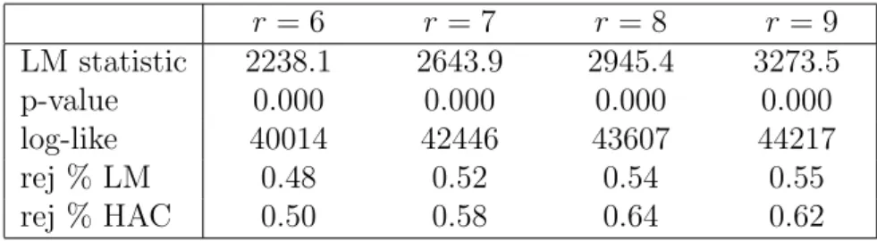
Results for r = 9 are provided in Table 8. The null hypothesis of no
9We are grateful to Giovanni Veronese for providing us with an updated version of that dataset.
10The New Eurocoin indicator is constructed based on 145 variables. The underlying dataset is larger. In their paper, Altissimo et al. (2007) select 145 series based on three criteria: a large time span, a high correlation and leading properties with respect to GDP growth and timely releases by statistical agencies. For our purposes, it is sufficient to use a balanced panel (between 1987:01 to 2007:06) which leaves us with 209 variables.
structural break is clearly rejected for both events by (the heteroscedasticity-robust version of) the LM test. Interestingly, the numbers tend to be larger for creatuib of the ECB than for the signing of the Maastricht treaty. The rejections rates are 0.18 and 0.63 for Maastricht and 0.40 and 0.60 for EMU when the tests are based on the LM and HAC test procedure, respectively. Have linkages become tighter or looser? We compare the commonality be-tween the pre-Maastricht, post-Maastricht and pre-EMU and the post-EMU periods and find no major change between the first and the second period when 9 factors explain 53.7% and 53.8% of the total variance, respectively. By contrast, the commonality increases to 55.7% in the third period which supports our finding of a more likely break in 1999:01 than in 1992:02.
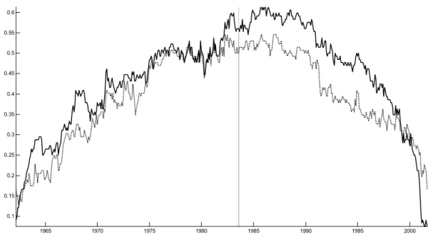
We can, again, assess whether the breaks have occurred only at the dates of the two specific events or before or after these dates. As shown in Figure 4, the null hypothesis of no structural break is, again, rejected for most of the sample period. The heteroscedasticity-robust version of the test indicates that the rejection rate is indeed highest (at 0.40) in 1999:01 (Figure 5). Figure 6 shows that the log likelihood reaches its global maximum around 1996/97, but values between 1996 and 1999 are barely distinguishable. One possible interpretation is that reforms and other public measures in the run-up of EMU may have altered comovements. Also, EMU has been anticipated and private agents may have adjusted their behaviour prior to the event. A third explanation is that the mid-1990s are also associated with a general worldwide acceleration of globalization, which may have tightened cyclical linkages between countries. Finally, as in the previous application, we find again a evidence for considerable heteroscedasticity in the factors.
Next, we investigate whether the events have affected certain countries more than others. We also formed groups of variables with similar eco-nomic content11 and examine whether certain groups of variables have expe-rienced structural breaks in the loadings while the loadings of other variables’ groups have remained stable. Table 9 shows the rejection rates for
individ-11“Industrial production” includes, besides industrial production, also retail sales, or-ders, export, imports, inventories, and car registrations. The “Inflation” group summarizes PPI as well as export and import price inflation. “Monetary and financial variables” con-tain interest rates, monetary aggregates, exchange rates, and stock prices. “Labor market” summarizes employment variables and wages as well as unit labor costs. Finally, survey expectations form the group “Surveys”.
ual countries. We only consider countries of which more than 10 variables were included in the dataset. Rejection rates are relatively high for both events for Spain and Italy, which are the countries with the lowest initial (1992) incomes12 and the highest inflation and long-term interest rates13 of the countries considered and, hence, the greatest needs to converge. Italy’s public debt was, in addition, quite elevated, compared to other countries.14 Table 9 also reports rejection rates for groups of variables. As for the overall tests, rejections rates for all groups are higher for EMU than for Maastricht. Our main finding is that, at the date of the creation of the ECB, rejection rates are relatively high for inflation as well as monetary and financial vari-ables. After all, EMU is a monetary event, and this result may therefore not be surprising. Maastricht has mainly caused breaks in industrial production series. Our results are insofar in line with Canova et al. (2006) that we also find some changes in the loadings which have occurred at the dates of the two events but also around these two events. By contrast, we identify clear structural breaks unlike Canova et al. (2006). The fact that their dataset does not include nominal variables may explain this difference between our and their finding. After all, the null hypothesis of no structural break is, at least for EMU, rejected relatively frequently for nominal variables.
6
Conclusions
Analyzing data sets with a large number of variables and time periods in-volves a severe risk that some of the model parameters are subject to struc-tural breaks. We show that strucstruc-tural breaks in the factor loadings may
12GDP per capita amounted to 25,536 and 21,103 US$ for Italy and Spain in 1992 and to 27,725, 26,608, 27,116, 28,168 US$ for Germany, France, Belgium, and the Netherlands, respectively, according to The Conference Board and Groningen Growth and Development Centre, Total Economy Database, January 2008.
13In 1992, year-on-year CPI inflation was at 5.3% and 5.9% in Italy and Spain and at 5.1%, 2.4%, 2.4%, 3.2% in Germany, France, Belgium, and the Netherlands, respec-tively. In 1992, the long-term interest rates were at 13.3% and 11.7% for Italy and Spain and at 7.9%, 8.6%, 8.7% and 8.1% for Germany, France, Belgium, and the Netherlands, respectively. Source: Economic Outlook, OECD.
14In 1992 the gross public debt as a percentage of GDP according to the Maastricht criterion as at 105.3% for Italy and at 45.9%, 42.1%, 38.8%, 128.5%, 77.4% for Spain, Germany, France, Belgium and the Netherlands, respectively. Source: Economic Outlook, OECD.
inflate the number of factors identified by the usual information criteria. Furthermore, we propose Chow type tests for structural breaks in factor models. It is shown that under the assumptions of an approximate factor model and if the number of variables is sufficiently large, the estimation er-ror of the common factors does not affect the asymptotic distribution of the Chow statistics. In other words, the PC estimator of the common factors is “super-consistent” with respect to the estimation of the factor loadings and, therefore, the usual Chow test can be applied to the factor model in a regression, where the unknown factors are replaced by principal components. Provided that the idiosyncratic components are mutually independent, i.e. under the assumption of a strict factor model, the variable-specific Chow statistics can be combined to test the joint null hypothesis of a common structural break. These tests can be generalized to dynamic factor models by adopting a GLS version of the test. This approach assumes a finite order autoregressive process for the idiosyncratic components, whereas no specific dynamic process needs to be specified for the common factors. Our Monte Carlo simulations suggest that the LM version outperforms the other variants of the test.
The LM test procedure is applied to two different settings. Our first em-pirical application uses a large US macroeconomic dataset provided by Stock and Watson (2005). We have tested whether the so called Great Moderation in the US (assuming the first quarter of 1984 as the starting date) coin-cides with structural breaks in the factor loadings. A lot of attention among researchers and policy makers has recently been directed to the Great Moder-ation. There is still some controversy about the sources (“good luck” versus structural changes including “good policy”), and we contribute to this de-bate. We find evidence of “dramatic changes” in the economy, reflected in significant breaks in the factor loadings, in the mid-1980s. By testing for breaks in the loadings of individual variables such as the Federal funds rate, inventories, industrial production in the durable and non-durable sectors, personal consumption expenditure and financial variables, we can assess the underlying sources of the structural change. We find support for the hypothe-sis that not a single but various factors have played an important role. These factors are, according to our analysis, changes in the conduct of monetary