by
Saman Muthukumarana
B.Sc., University of Sri Jayewardenepura, Sri Lanka, 2002 M.Sc., Simon Fraser University, 2007
a Thesis submitted in partial fulfillment of the requirements for the degree of
Doctor of Philosophy in the Department
of
Statistics and Actuarial Science
c
Saman Muthukumarana 2010 SIMON FRASER UNIVERSITY
Summer 2010
All rights reserved. This work may not be reproduced in whole or in part, by photocopy or other means, without the permission of the author.
APPROVAL
Name:
Saman Muthukumarana
Degree:
Doctor of Philosophy
Title of Thesis:
Bayesian Methods and Applications using WinBUGS
Examining Committee:
Dr. Derek Bingham
Chair
Dr. Tim Swartz, Senior Supervisor
Dr. Paramjit Gill, Supervisor
Dr. Carl Schwarz, Supervisor
Dr. Jiguo Cao, SFU Examiner
Dr. Paul Gustafson, External Examiner
University of British Columbia
JUN 2 82010
Date Approved:
••
Last revision: Spring 09
Declaration of
Partial Copyright Licence
The author, whose copyright is declared on the title page of this work, has granted to Simon Fraser University the right to lend this thesis, project or extended essay to users of the Simon Fraser University Library, and to make partial or single copies only for such users or in response to a request from the library of any other university, or other educational institution, on its own behalf or for one of its users. The author has further granted permission to Simon Fraser University to keep or make a digital copy for use in its circulating collection (currently available to the public at the “Institutional Repository” link of the SFU Library website <www.lib.sfu.ca> at: <http://ir.lib.sfu.ca/handle/1892/112>) and, without changing the content, to translate the thesis/project or extended essays, if technically possible, to any medium or format for the purpose of preservation of the digital work.
The author has further agreed that permission for multiple copying of this work for scholarly purposes may be granted by either the author or the Dean of Graduate Studies.
It is understood that copying or publication of this work for financial gain shall not be allowed without the author’s written permission.
Permission for public performance, or limited permission for private scholarly use, of any multimedia materials forming part of this work, may have been granted by the author. This information may be found on the separately catalogued multimedia material and in the signed Partial Copyright Licence.
While licensing SFU to permit the above uses, the author retains copyright in the thesis, project or extended essays, including the right to change the work for subsequent purposes, including editing and publishing the work in whole or in part, and licensing other parties, as the author may desire.
The original Partial Copyright Licence attesting to these terms, and signed by this author, may be found in the original bound copy of this work, retained in the Simon Fraser University Archive.
Simon Fraser University Library Burnaby, BC, Canada
In Bayesian statistics we are interested in the posterior distribution of parameters. In simple cases we can derive analytical expressions for the posterior. However in most situations, the posterior expectations cannot be calculated analytically due to the complexity of the integrals. This thesis develops some new methodologies for applied problems which deal with multidimensional parameters, complex model structures and complex likelihood functions. The first project is concerned with the simulation of one-day cricket matches. Given that only a finite number of outcomes can occur on each ball, a discrete generator on a finite set is developed where the outcome probabilities are estimated from historical data. The probabilities depend on the batsman, the bowler, the number of wickets lost, the number of balls bowled and the innings. The proposed simulator appears to do a reasonable job at producing realistic results. The simulator allows investigators to address complex questions involving one-day cricket matches.
The second project investigates the suitability of Dirichlet process priors in the Bayesian analysis of network data. Dirichlet process priors allow the researcher to weaken prior as-sumptions by going from a parametric to a semiparametric framework. This is important in the analysis of network data where complex nodal relationships rarely allow a researcher the confidence in assigning parametric priors. The Dirichlet process also provides a clus-tering mechanism which is often suitable for network data where groups of individuals in a network can be thought of as arising from the same cohort. The approach is highlighted on two network models and implemented using WinBUGS.
The third project develops a Bayesian latent variable model to analyze ordinal survey data. The data are viewed as multivariate responses arising from a class of continuous
that have a Dirichlet process as their joint prior distribution. The proposed mechanism adjusts for classes of personality traits. As the resulting posterior distribution is complex and high-dimensional, posterior expectations are approximated by MCMC methods. The methodology is tested through simulation studies and illustrated using student feedback data from course evaluations at Simon Fraser University.
Keywords: Bayesian latent variable models, Clustering, Dirichlet process, Markov chain Monte Carlo, Simulation, WinBUGS
There are many people who helped me to be successful in my academic career over last few years at SFU. It is impossible to name and thank all of them in a page.
I’m deeply indebted to my senior supervisor Dr. Tim Swartz for mentoring me in limitless ways. I’m grateful for the freedom he gave me to explore new directions and understanding and nurturing my research interests. The full and continuous financial support provided during the last five years allowed me to entirely focus on my studies. I was very lucky to have such an amazing mentor in my life.
A big thank-you goes to Dr. Paramjit Gill and Dr. Pulak Ghosh for having stimulating discussions which helped me accomplish my goals. I also want to thank Dr. CJS for giving me the opening to work on the CJS model which yielded my first paper to appear in CJS. There are many others in the Department of Statistics and Actuarial Science who helped in many ways during my life at SFU. Special thanks to Robin Insley, Dr. Richard Lockhart, Dr. Joan Hu, Dr. Jinko Graham, Dr. Brad McNeney, Dr. Charmaine Dean, Dr. Derek Bingham, Dr. Tom Loughin and Ian Bercovitz. I also thank Dr. Jiguo Cao and Dr. Paul Gustafson for their comments and suggestions on the thesis. I must also thank Dr. Sarath Banneheka for initiating my interest in Statistics.
I offer my sincere gratitude to Sadika, Kelly and Charlene for your kindness, help and promptness on all the matters. I would also like to thank all of the graduate students for their friendship. Especially: Ryan, Matt, Crystal, Pritam, Kyle, Dean, Wei, Kelly, Jean, Carolyn, Simon, Chunfang, Elizabeth, Lihui, Wendell, Cindy, Vivien, Joslin, Rianka, Jervyn and many more . . . . Finally, and most importantly, I appreciate Aruni for her patient support and sacrifices. This would not have been finished without her understanding.
Approval ii
Abstract iii
Acknowledgements v
Contents vi
List of Figures viii
List of Tables x
1 Introduction 1
1.1 The Bayesian paradigm . . . 1
1.2 MCMC methods using WinBUGS . . . 5
1.3 Organization of the thesis . . . 6
1.3.1 One-day international cricket . . . 6
1.3.2 Social network models . . . 7
1.3.3 Ordinal survey data . . . 8
2 Modelling and Simulation for One-Day Cricket 9 2.1 Introduction . . . 9
2.2 Simulation . . . 12
2.3 Modelling . . . 15
2.4 Generating runs in the second innings . . . 22
2.5 Testing model adequacy . . . 26
2.7 Discussion . . . 35
3 A Bayesian Approach to Network Models 37 3.1 Introduction . . . 37
3.2 The Dirichlet process . . . 39
3.3 Example 1: A social relations model . . . 41
3.4 Example 2: A binary network model . . . 47
3.5 Example 3: A Simulation Study . . . 51
3.6 Discussion . . . 53
4 Bayesian Analysis of Ordinal Survey Data 54 4.1 Introduction . . . 54
4.2 Model development . . . 56
4.3 Computation . . . 60
4.4 Examples . . . 61
4.4.1 Course evaluation survey data . . . 61
4.4.2 Simulated data . . . 65 4.5 Goodness-of-Fit . . . 67 4.6 Discussion . . . 70 5 Discussion 72 Bibliography 74 Appendices 80
A WinBUGS Code for the ODI Cricket Model 81
B WinBUGS Code for the Network Model 83
C WinBUGS Code for the Ordinal Survey Model 86
D R Code for the Prior Predictive Simulation 89
2.1 Logistic density function and typical parameters for the model in (5). . . . 19 2.2 QQ plot corresponding to first innings runs for Sri Lanka batting against India. 30 2.3 Histogram of the length of the partnership (in overs) of the untested opening
partnership of Alastair Cook and Ian Bell. . . 32 3.1 Posterior means of the (αi, βi) pairs under the normal prior in Example 1. . 43 3.2 Posterior means of the (αi, βi) pairs under the DP prior in Example 1. . . . 44 3.3 Posterior box plots of theαi’s under the DP prior in Example 1. . . 45 3.4 Posterior box plots of theβi’s under the DP prior in Example 1. . . 46 3.5 Plot of out-degree versus in-degree for the 71 lawyers in Example 2 where the
lawyers labelled with triangles are associates and the lawyers labelled with circles are partners. . . 49 3.6 Plot of pairwise clustering of the 71 lawyers based on the DP model in
Ex-ample 2. Black (white) squares indicate posterior probabilities of clustering greater than (less than) 0.5. Labels 1-36 correspond to partners and labels 37-71 correspond to associates. . . 50 4.1 Plot of the posterior means of the personality trait parameters (ai, bi) for the
actual SFU survey data. . . 64 4.2 Estimate of the posterior density ofµ1 for the actual SFU survey data. . . . 65
4.3 Trace plot forµ1 based on the MCMC simulation for the actual SFU survey
data. . . 65 4.4 Autocorrelation plot for µ1 based on MCMC simulation for the actual SFU
survey data. . . 66
simulated data example. . . 68 4.6 Histogram corresponding to the (N+12 )= 210 Euclidean distances with respect
to the prior-predictive check for the actual SFU survey data. . . 70
2.1 The number of ODI matches for which data were collected on the ICC teams. 16 2.2 The nine first innings situations where aggressiveness is assumed constant.
The fourth column provides the percentage of balls in the dataset that cor-respond to the given situation. . . 20 2.3 Batting probabilitiespfor various states and the expected number of runs per
overE(R) where CM denotes the Cook/McGrath matchup and CH denotes the Cook/Hossain matchup. . . 28 2.4 Second innings batting probabilitiesp0 and the expected number of runs per
over for the Cook/Hossain matchup when Bangladesh has scored f = 250 runs in the first innings. In the second innings,w= 3 wickets have been lost, ball b= 183 is about to be bowled and England has scoredsruns. . . 29 2.5 Estimated probabilities of the row team defeating the column team where
the row team corresponds to the team batting first. The final column are the row averages and correspond to the average probabilities of winning when batting in the first innings. The final row are the average probabilities of winning when batting in the second innings. . . 34 4.1 Estimates of posterior means and posterior standard deviations for the actual
SFU survey data. . . 63 4.2 Estimates of posterior means and standard deviations in the simulated data
example. . . 67
Introduction
1.1
The Bayesian paradigm
The Bayesian framework was introduced by the Reverand Thomas Bayes (1702-1761) and Bayesian estimation was first used by LaPlace in 1786. Today, Bayesian statistics is widely used by researchers in diverse fields due to significant computational advancements includ-ing MCMC, BUGS and WinBUGS software. Researchers in many fields have embraced the Bayesian approach due to its capacity to handle complexity in real world problems. The Bayesian approach has many attractive features over frequentist statistics. In par-ticular, missing data and latent variables often pose no difficulties in Bayesian analyses. The Bayesian approach also provides a way to include expert prior knowledge concerning parameters of interest.
In a frequentist approach, the data are taken as random while parameters are consid-ered fixed. In a Bayesian approach, parameters themselves follow a probability distribution. Furthermore, parameters may be model parameters, missing data or events that are not observed (latent). Frequentist methods also typically rely upon approximations and asymp-totic results and these cases are only valid for large samples. Moreover, frequentist methods often replace missing data with guesses and then analyze the data as though the guesses were known or else delete records for subjects that have even one missing value.
This thesis develops some new methodologies for applied problems which deal with multidimensional parameters, complex model structures, latent variables, missing data and
complex likelihood functions. The following components are required in order to carry out a Bayesian analysis:
• the prior distribution of the parameters • the likelihood corresponding to the data
A prior distribution of a parameter quantifies the uncertainty about the parameter before the data are observed. It is important that priors are selected such that they rep-resent the best knowledge about parameters. If it is not possible, we may be able to use non-informative priors which often produce useful results provided that there is sufficient information in the likelihood. Recall that Bayes formula gives the posterior distribution
π(θ|y) = f(y|θf()yπ)(θ)
where f(y |θ) is the likelihood, π(θ) is the prior density or probability mass function and f(y) is the inverse normalizing constant given by
f(y) =
Z
f(y|θ)π(θ)dθ.
Here θ can be a scalar or a vector of parameters and y is the vector of observed data. In many Bayesian analyses, it is not necessary to calculate the inverse normalizing constant.
In order to perform inferences about components of θ, one is typically faced with high-dimensional integrals. For example, the posterior mean of θ1 is given by
E(θ1 |y) = R θ1π(θ1 |y)dθ1 = R θ1 R π(θ|y)dθ(−1) dθ1
where θ(−1) is the vector θ with θ1 removed. In simple models, integration problems can
sometimes be avoided by choosing particular types of priors. If the prior and likelihood are natural conjugate distributions, then the posterior is in the same family as the prior and integrals may be tractable. For more complex models, the calculation of integrals is often difficult and sometimes impossible. Sometimes numerical approaches such as quadrature and Laplaces method can be used to approximate the expectations. Evans and Swartz
(1995) provide a discussion of the major techniques available for the approximation of integrals in statistics.
In theory, the functional form of the posterior density provides a complete description of the uncertainty in the parameters. However, to gain insight with respect to the posterior, posterior expectations in the form of integrals are typically desired. In the case of complex posteriors, the integrals can not be evaluated analytically. Instead, simulation procedures are often used to sample variates from the posterior. In a simulation context, sampling directly from the posterior may not be easy in complex problems and there are some alter-native sampling strategies which may be useful. The most widely used sampling methods are
• importance sampling
• Markov chain Monte Carlo (MCMC)
In Evans and Swartz (1995), these two methods are discussed where Markov chain methods are recommended for high-dimensional problems such as in the problems considered in this thesis. In MCMC, variates are drawn from a distribution which has the posterior distribution as its equilibrium distribution. In MCMC, output may be averaged to obtain approximations to posterior expectations. A Markov chain is a random process where the variate at iterationidepends only on the variate at iterationi−1. Various algorithms have been developed to implement MCMC. The most popular algorithms are
• Metropolis-Hastings • Gibbs sampling
Given previously generated variates θ(1), . . . ,θ(k−1), the Metropolis-Hastings algorithm proceeds by generatingθ∗ from a proposal densityq(θ, θ(k−1)). Note that the proposal may depend on the previous variateθ(k−1). This generated valueθ∗ is accepted (ieθk =θ∗) with probability min 1, q(θ (k−1), θ∗)π(θ∗ |y) q(θ∗, θ(k−1))π(θ(k−1)|y) ! . (1.1)
If θ∗ is not accepted, then θ(k) = θ(k−1). The rate at which the new values are accepted
is called the acceptance rate. The process is repeated to obtain a sequence θ(1), θ(2), . . . where θ(k) is approximately a realization from the posterior for sufficiently large k. The
Metropolis-Hastings algorithm requires an initial valueθ(0)in order to start the simulation. The choice of initial value may effect the rate of convergence of the algorithm. Initial values which are far away from the range covered by the posterior distribution often lead to chains that take more iterations to attain convergence.
The Gibbs sampling algorithm is a special case of the Metropolis-Hastings algorithm in which samples are drawn by turning the multivariate problem into a sequence of lower-dimensional problems. In Gibbs sampling, parameters are generated from distributions with a 100% acceptance rate.
Fortunately, the software package WinBUGS implements MCMC methods using the Metropolis-Hastings or Gibbs algorithm. The default option in WinBUGS for well behaved models with log concave densities is the Gibbs sampling algorithm. However, Metropolis-Hastings is invoked for nonstandard models. In WinBUGS, we need only specify the like-lihood, the prior, the observed data and the initial values. WinBUGS then produces an appropriate Markov chain. Clearly, WinBUGS requires much less MCMC programming than if one was to program the MCMC simulations.
However, we need to make sure that a sequence has converged before inferences are obtained. The number of iterations taken for the practical convergence to the stationary distribution depends on various factors including
• the complexity of the model (models with few parameters generally converge faster) • whether the prior and likelihood are conjugate
• the closeness of initial values to their respective posterior means • the parameterization of the problem
• the sampling scheme adopted
The number of iterations prior to convergence is called the burn-in, and we typically discard these variates for the purpose of inference. WinBUGS provides several statistics
and graphical tools to check the convergence of Markov chains. Brooks and Gelman (1997) discuss some these methods.
1.2
MCMC methods using WinBUGS
WinBUGS is a product of the BUGS (Bayesian Inference Using Gibbs Sampling) project which is a joint program of the Medical Research Council of Biostatistics Unit at Cambridge University and the Department of Epidemiology and Public Health of Imperial College at St. Mary’s Hospital in London. The software is freely distributed from their web page at (www.mrc-bsu.cam.ac.uk/bugs). Models can be implemented in two ways:
• using the script language
• using the graphical feature, DoodleBUGS which allows the specification of models in terms of a directed graph
The range of model types that can be fitted in WinBUGS is very large. A wide variety of linear and nonlinear models, including the standard set of generalised linear models, spatial models and latent variable models can be fitted. In addition, a range of prior distributions is available with standard defaults. We believe that WinBUGS is a very handy tool in fitting complex models although it is a difficult and frustrating package to master. One of the main issues of WinBUGS is that there is a great amount of embedded statistical theory associated with MCMC. Lack of knowledge of relevant theory can sometimes lead inexperienced users into a state of false security. There are other issues associated with Bayesian modelling, such as choice of priors and initial values that are also relevant. Bayesian analysis using WinBUGS requires three major tasks as follows:
• model specification • running the model
In WinBUGS, there are three types of nodes referred to as constant, stochastic and deterministic. Constant nodes are used to declare constant terms. Stochastic nodes repre-sent data or parameters that are assigned a distribution. Currently WinBUGS provides 23 familiar distributions. Deterministic nodes are logical expressions of other nodes. Logical expressions can be built using the operators +, -, *, / and various WinBUGS functions. Note that WinBUGS has some special syntax which differs from other languages such as Splus and C++. As an example, WinBUGS requires that each node appear exactly once on the left hand side of an equation. During and after MCMC simulation, WinBUGS provides several numerical and graphical summaries for the parameters. The dynamic trace plots for each parameter, Brooks-Gelman-Rubin convergence statistics (Brooks and Gelman 1997) and the autocorrelation plots of the sequences are handy tools for investigating conver-gence to the equilibrium distribution. The Brooks-Gelman-Rubin converconver-gence statistics are graphical tools for assessing convergence of multiple chains to the same distribution. Since the simulations from multiple chains are independent, evidence of convergence is based on the equality of within chain variability and between chain variability. CODA (Conver-gence Output and Diagnostic Analysis) software is also easily accessible from other software platforms for further analysis.
1.3
Organization of the thesis
This thesis involves model development, computation and inferences associated with three applied problems which deal with multidimensional parameters, complex model structures and complex likelihood functions. The commonality of the three problems is that they each involve a Bayesian analysis implemented via WinBUGS. Chapters 2, 3 and 4 individually correspond to one of the three problems. Each chapter is written in a stand-alone fashion and corresponds closely to the technical paper upon which it is based.
1.3.1 One-day international cricket
Chapter 2 is concerned with the simulation of one-day cricket matches. In one day interna-tional cricket matches, there are an endless number of questions that are not amenable to
experimentation or direct analysis but could be easily addressed via simulation. A good sim-ulator for ODI cricket is required to provide reliable answers to such questions. Given that only a finite number of outcomes can occur on each ball that is bowled, a discrete generator on a finite set is developed via a Bayesian latent variable model where the outcome probabil-ities are estimated from historical data involving one-day international cricket matches. The probabilities depend on the batsman, the bowler, the number of wickets lost, the number of balls bowled and the innings. The proposed simulator appears to do a reasonable job at producing realistic results. The simulator allows investigators to address complex questions involving one-day cricket matches. This work was published in the Canadian Journal of Statistics in 2009.
1.3.2 Social network models
Chapter 3 considers the use of Dirichlet process priors in the statistical analysis of social net-work data. A social netnet-work is a data structure which considers relationships (ties) between nodes. The nodes can be people, groups, organizations, cities, countries, etc. The ties can be transfer of goods, money, information, political support, friendship, etc. There are many applications of social network analysis such as citation analysis which identifies influential papers in a research area, dynamics of the spread of disease in epidemiology, identifying most effective areas for product/service distributions in business and telecommunications and coalition formation dynamics in political science. In social networks, it is possible that there are partitions of the data such that data within classes are similar. There may also be some nodes that appear to play network roles or some may be isolated from groups. These types of complex nodal relationships rarely allow a researcher confidence in assigning parametric priors. Dirichlet process priors allow the researcher to weaken prior assumptions by going from a parametric to a semiparametric framework. In addition, the standard nor-mality assumption does not allow outlying subjects and also conclusions may be sensitive to violations from normality. The normality assumption is relaxed by the use of Dirichlet process priors. The Dirichlet process has a secondary benefit due to the fact that its sup-port is restricted to discrete distributions. This provides a clustering mechanism which is often suitable for network data where groups of individuals in a network can be thought
of as arising from the same cohort. Most importantly, in the proposed model, clustering takes place as a part of the model and data decide the clustering structure. The approach is highlighted on two network models. This work has been accepted for publication in the Australian and New Zealand Journal of Statistics (2010).
1.3.3 Ordinal survey data
Chapter 4 presents a Bayesian latent variable model used to analyze ordinal response survey data. The ordinal response data are viewed as multivariate responses arising from a class of continuous latent variables with known cut-points. Each respondent is characterized by two parameters that have a Dirichlet process as their joint prior distribution. The key aspect of the Dirichlet process in this application is that the personality trait parameters of the survey respondents have support on a discrete space and this enables the clustering of personality types. The proposed mechanism adjusts for classes of personality traits. As the resulting posterior distribution is complex and high-dimensional, posterior expectations are approximated by MCMC methods. As a by-product of the proposed methodology, one can identify survey questions where the corresponding performance has been poor or exceptional. The methodology is tested through simulation studies and illustrated using student feedback data in teaching and course evaluations at Simon Fraser University (SFU). Goodness-of fit is investigated using prior predictive methods. This work has been submitted and is currently under review.
The thesis concludes with a discussion in chapter 5. The WinBUGS code for the three problems is provided in Appendix A, B and C respectively. In Appendix D, R code is provided which is used in the goodness-of-fit approach from chapter 4.
Modelling and Simulation for
One-Day Cricket
2.1
Introduction
Simulation is a practical and powerful tool that has been used in a wide range of disci-plines to investigate complex systems. When a simulation model is available, it is typically straightforward to address questions concerning the occurrence of various phenomena. One simply carries out repeated simulations and observes the frequency which the phenomena occur.
In one-day international (ODI) cricket, there are an endless number of questions that are not amenable to experimentation or direct analysis but could be easily addressed via simulation. For example, on average, would England benefit from increasing the number of runs scored by changing the batting order of their third and sixth batsmen? As another example, what percentage of time would India be expected to score more than 350 runs versus Australia in the first innings?
To provide reliable answers to questions such as these, a good simulator for one-day cricket matches is required. Surprisingly, the development of simulators for one-day cricket is a topic that has not been vigorously pursued by academics. In the pre-computer days, Elderton (1945) and Wood (1945) fit the geometric distribution to individual runs scored based on results from test cricket. Kimber and Hansford (1993) argue against the geometric
distribution and obtain probabilities for selected ranges of individual scores in test cricket using product-limit estimators. More recently, Dyte (1998) simulates batting outcomes between a specified test batsman and bowler using career batting and bowling averages as the key inputs without regard to the state of the match (e.g. the score, the number of wickets lost, the number of overs completed). Bailey and Clarke (2004, 2006) investigate the impact of various factors on the outcome of ODI cricket matches. Some of the more prominent factors include home ground advantage, team quality (class) and current form. Their analysis is based on the modelling of runs using the normal distribution.
In a non-academic setting, there are currently more than 100 cricket games that have been developed for use on personal computers and gaming stations where some of the games rely on simulation techniques (see www.cricketgames.com/games/index.htm for a comprehensive survey of games and reviews). However, in all of the games that we have inspected, the details of the simulation procedures have not been revealed. Moreover, the games that we have inspected suffer in various ways from a lack of realism.
One-day cricket was introduced in the 1960’s as an alternative to traditional forms of cricket that may take up to five days to complete. With more aggressive batting, colourful uniforms and fewer matches ending in draws, one-day cricket has become extremely popular. The ultimate event in ODI cricket takes place every four years where the World Cup of Cricket is contested.
One-day cricket has some similarities with the sport of baseball. The game is played between two teams of 11 players where a batting team attempts to score runs against a fielding team until the first innings terminate. At this stage, the fielding team goes “to bat” and attempts to score more runs before the second innings terminate. A bowler on the fielding team “bowls” balls in groups of six referred to asovers. Bowling takes place only from one end of the pitch during an over, and the bowling end changes on the subsequent over. A batsman on the batting team faces a bowled ball with a bat and attempts to score runs. Runs are scored by running between two stumps located at opposite ends of the pitch. The running aspect involves two batsmen known as a partnership where each partner is running to the opposite stump. They may score 0, . . . ,6 runs according to the number of traversals between the stumps. Therefore, the batsman in the partnership who
is located at the batting end faces the next ball. An innings terminates when either 50 overs are completed or 10wicketsare lost. A loss of a wicket can occur in various ways with the three most common being (i) a ball is caught in midair after having been batted, (ii) a bowled ball hits the stump located behind the batsman, and (iii) a batsman is run-out
before reaching the nearest stump. When a wicket is lost, a new batsman is introduced in the batting order. This is a very brief introduction to the rules of one-day cricket, and more information is provided in the paper as required. More detail on the rules (laws) of cricket is available from the Lord’s website (www.lords.org).
In this paper, we develop a simulator for one-day cricket matches. The approach ex-tends the work of Swartz, Gill, Beaudoin and de Silva (2006) who investigate the problem of optimal batting orders in one-day cricket for the first innings. Whereas the model used in Swartz et al. (2006) ignores the effect of bowlers, the model used in this paper is more realistic in that specific batsman/bowler combinations are considered. In addition, we now provide a method of generating runs in the second innings. Given that only a finite num-ber of outcomes can occur on each ball that is bowled, a discrete generator on a finite set is developed where the outcome probabilities are estimated from historical data involving ODI cricket matches. The probabilities depend on the batsman, the bowler, the number of wickets lost, the number of balls bowled and the current score of the match. The probabil-ities are obtained using a Bayesian latent variable model which is fitted using WinBUGS software (Spiegelhalter, Thomas, Best and Lunn 2004).
In Section 2.2, we develop a simulator for ODI cricket which is based upon a Bayesian latent variable model. Particular attention is given to second innings batting where the state of the match (e.g. score, wickets, overs) affects the aggressiveness of batsmen. In Section 2.3, the simulator is constructed using data from recent ODI matches. The methodology is developed for generating runs in the second innings in Section 2.4. In Section 2.5, we consider the adequacy of the approach by comparing simulated results against actual data. In Section 2.6, we demonstrate how the simulator can be used to address questions of interest. We conclude with a short discussion in Section 2.7.
2.2
Simulation
We consider the simulation of runs in the first innings for predetermined batting and bowling orders. We initially investigate the first innings runs since second innings strategies are affected by the number of runs scored in the first innings. By a predetermined batting and bowling order, we mean that a set of rules has been put in place which dictates the batsman and bowler at any given point in the match. These rules could be simple such as maintaining a fixed batting and bowling order. The rules for determining batting and bowling orders could also be very complex. For example, the rules could be Markovian in nature where a specified bowler may be substituted at a state in the match dependent upon the number of wickets lost, the number of overs, the number of runs and the current batsmen. The key point is that they need to be specified in advance for the purpose of simulation.
In one-day cricket, there are a finite number of outcomes arising from each ball bowled. Suppose that the first innings terminate on the m-th ball bowled wherem≤300. Ignoring certain rare events (such as scoring 5 runs), and temporarily ignoring wide-balls and no-balls, letXb denote the outcome of theb-th ball bowled,b= 1, . . . , mwhere
Xb= 1 if a wicket is taken
2 if the batsman scores 0 runs 3 if the batsman scores 1 run 4 if the batsman scores 2 runs 5 if the batsman scores 3 runs 6 if the batsman scores 4 runs 7 if the batsman scores 6 runs
(2.1)
and set Xm+1 =· · · =X300 = 0. Note that the coding in (2.1) includes the possibility of
scoring due to byes and and leg byes. Byes and leg byes occur when the batsman has not hit the ball with his bat but decides to run.
Using square brackets to generically denote probability mass functions, the joint distri-bution ofX1, . . . , X300 can be written as
where we defineX0= 0 for notational convenience. Note that the conditional probabilities
in (2.2) suggest that the scoring distribution for a given ball depends on the scoring up to that point in time in the first innings. The proposed simulation algorithm is facilitated by the structure in (2.2) whereby the first outcome X1 is generated for the first ball bowled,
then the second outcome X2 is generated for the second ball bowled conditional on X1.
The first innings continue until either the overs are completed (b= 300) or all wickets are lost (wickets=10). Letv denote the probability of a wide-ball or a no-ball. The simulation algorithm generates a uniform(0,1) random variableu, and if u < v, this signals a wide-ball or no-ball condition. In this case, a single run is added to the batting team but the ball is not counted. In addition, further runs may be scored on the no-ball or wide-ball according to the probabilityφkfor thek-th outcome,k= 1, . . . ,7. The following simulation algorithm generates the number of runs R scored in the first innings:
wickets = 0 R= 0 forb= 1, . . . ,300 if wickets = 10 then Xb = 0 else generateu∼uniform(0,1) ? ifu < v then generate Y ∼multinomial(1, φ1, . . . , φ7)
R←R+ 1 +I(Y = 3) + 2I(Y = 4) + 3I(Y = 5) + 4I(Y = 6) + 6I(Y = 7) goto step?
else
generate Xb ∼[Xb |X0, . . . , Xb−1]
R←R+I(Xb = 3) + 2I(Xb = 4) + 3I(Xb = 5) + 4I(Xb= 6) + 6I(Xb= 7) wickets←wickets +I(Xb = 1)
For the sake of simplicity, the above algorithm does not distinguish a run-out from other forms of wickets. Runs may still be accumulated on a ball prior to a run-out, and the dismissed batsman may be either of the two batsmen in the partnership. We remark that we have estimated the probability of run-outs and have accounted for run-outs in our Fortran implementation of the above algorithm. The proposed simulation algorithm is simple and requires only that we be able to generate from the multinomial(1, φ1, . . . , φ7)
distribution and the conditional finite discrete distributions given by [Xb | X0, . . . , Xb−1].
In the following subsection, we describe a method to compute the conditional distributions by modelling ball by ball outcomes in one-day cricket matches.
2.3
Modelling
The conditional distributions [Xb |X0, . . . , Xb−1] depend on many factors including
• the batsman • the bowler
• the number of wickets lost • the number of balls bowled • the current score of the match • the opposing team
• the location of the match • the coach’s advice
• the condition of the pitch, etc.
For the first innings, we consider the first four factors and define pijwbk as the probability corresponding to outcome k = 1, . . . ,7 as described in (2.1), where the the i-th batsman, i = 1, . . . , I faces the j-th bowler, j = 1, . . . , J when w = 0, . . . ,9 wickets have been lost and theb-th ball is about to be bowled, b= 1, . . . ,300. Since wide-balls and no-balls have been excluded as possible outcomes of Xb, we have Pkpijwbk = 1 for all i, j, w, b. With estimates ˆpijwbk, the simulation algorithm generates outcomes according to
Prob(Xb=k|X0, . . . , Xb−1) = ˆpijwbk. (2.3) Our data are based on 472 ODI matches from January 2001 until July 2006 amongst the 10 full member nations of the International Cricket Council (ICC). These matches are those for which ball by ball commentary is available on the Cricinfo website (www.cricinfo.com) and include almost all matches amongst the 10 nations during the specified time period. We note that a Powerplay rule was introduced for a 10 month trial period beginning August 2005 and the Supersub rule was introduced for a portion of the trial period. Although we believe that these temporary rules had some effect on scoring, we do not account for the presence and absence of the temporary rules in our modelling. In the 472 matches, 257922 balls were bowled involving I = 435 batsman and J = 360 bowlers. In the first innings,
Table 2.1: The number of ODI matches for which data were collected on the ICC teams.
ICC Nation Number of Matches
Australia 106 Bangladesh 48 England 89 India 125 New Zealand 94 Pakistan 108 South Africa 101 Sri Lanka 118 West Indies 77 Zimbabwe 78
138439 balls were bowled. In Table 2.1, we record the number of matches for which data were collected on the ICC teams. Excepting Bangladesh, we observe that there is reasonable balance in the number of matches played.
Over these matches, we calculate ˆv= 8289/257922 = 0.032 as the total number of wide-balls and no-wide-balls divided by the total number of wide-balls bowled. The conditional probabilities φk are similarly estimated by frequencies.
Before describing the model used in the estimation of pijwbk, we offer some preliminary comments based on our experience in fitting numerous models over several years. Most importantly, our goal is to obtain a model which fits well and provides a realistic simulator. With regard to estimation and prediction, there are many situations for which data do not exist. For example, a given batsman i may never have faced a given bowler j in the third over when two wickets are lost. To predict what may happen in these situations it is necessary to borrow information from similar situations. For example, it is relevant in the above problem to consider how other batsman/bowler combinations fared in the third over when two wickets are lost, and it is also relevant to consider how batsman i fared against bowler j in other stages of a match. With nearly 1000 batsmen and bowlers, our
experience suggests that it is not a good idea to have multiple parameters for each batsman and bowler since this leads to excessive parameterization. When the number of parameters is excessive, computation may be overwhelming and unreliable estimates may arise. We strive for parsimonious model building, assigning only a single parameter to each batsman and assigning only a single parameter to each bowler.
To obtain the estimates ˆpijwbk in (2.3), we develop a Bayesian latent variable model which is related to the classical cumulative-logit models for ordinal responses (Agresti 2002). We initially assume that batting is taking place in the first innings and we temporarily ignore the state of the first innings (e.g. the number of overs completed and the number of wickets lost). We imagine that there is a latent continuous variableU which describes the “quality” of the batting outcome. For example, one might imagine that a ball batted near a fielder has a lower rating than a similar ball batted slightly further away from the fielder. AlthoughU is unobserved (latent), there is an observed data variableXwhich is related toU as follows:
X = 1 (dismissal) ↔ a0 < U ≤a1 X = 2 (0 runs) ↔ a1 < U ≤a2 X = 3 (1 runs) ↔ a2 < U ≤a3 X = 4 (2 runs) ↔ a3 < U ≤a4 X = 5 (3 runs) ↔ a4 < U ≤a5 X = 6 (4 runs) ↔ a5 < U ≤a6 X = 7 (6 runs) ↔ a6 < U ≤a7
where −∞=a0 < a1 <· · · < a6 < a7 =∞. Note that increasing values of X correspond
to higher quality of batting outcomes and thata1, . . . , a6 are unknown parameters.
We now define a single batsman characteristic µ(1)i for the i-th batsman and a single bowler characteristic µ(2)j for the j-th bowler. We assume that the quality of the batting outcomeU is expressed as
U =µ(1)i −µ(2)j + (2.4)
whereµ(1) = 0 represents an average batsmen,µ(2)= 0 represents an average bowler and is a random variable whose distribution determines the quality of the batting outcome for an average batsman and an average bowler. From (2.4), we observe that a good batsman
(µ(1)i >0) increases the quality of the batting outcome. Similarly, a good bowler (µ(2)j >0) decreases the quality of the batting outcome. Letting F denote the distribution function of , we write Prob(X ≤k) = Prob(U ≤ak) = Prob(µ(1)i −µ(2)j +≤ak) = Prob(≤ak−µ(1)i +µ (2) j ) = F(ak−µ(1)i +µ(2)j ) (2.5)
for the batting outcomek= 1, . . . ,7.
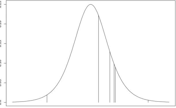
To gain a better appreciation of the model given by (2.5), refer to Figure 2.1 where the density function of the logistic distribution (i.e. F() = 1/(1 + exp(−))) has been chosen using typical values of a1, . . . , a6. The logistic distribution is symmetric about 0 and has
longer tails than the normal distribution. We observe that the area under the density function between ak−1 and ak corresponds to the probability that X = k. The effect of better batsmen (µ(1)i > 0) and weaker bowlers (µ(2)j < 0) causes a simultaneous leftward shift in the vertical lines and hence decreases the probability of dismissal and increases the probability of scoring 6 runs.
A difficulty with the model given by (2.5) is that it does not account for the variability in aggressiveness which batsmen display during the first innings. For example, it is well-known that batsmen become more aggressive in the final overs if few wickets have been lost. Increasing aggressiveness corresponds to an increase in the probability of dismissal (k= 1), a decrease in the probability of scoring 0 runs (k = 2) and an increase in the probability of scoring 6 runs (k = 7). The effect of increasing aggressiveness on the remaining four outcomesk= 3,4,5,6 is not as obvious and is situation dependent. Note that aggressiveness is a characteristic that affects the parametersakand is different from the quality of batsmen µ(1)i and the quality of bowlers µ(2)j . In the spirit of parsimonious model building, in Table 2.2 we propose 9 situations where aggressiveness is assumed constant. Situations 1, 2 and 3 are motivated by the fielding restriction which is in place during the first 15 overs. We view overs 16-35 as the middle period of the first innings where any change in aggressiveness is due to wickets lost. The final period of the first innings (overs 36-50) can lead to very aggressive batting if few wickets are lost. We note that situations 4, 7 and 8 are particularly rare and
0.0 0.05 0.10 0.15 0.20 0.25
a1=−3.91 a2=0.70 . . . a6=5.14
Figure 2.1: Logistic density function and typical parameters for the model in (5). the parameters corresponding to these situations may not be well estimated. However, this is not a great concern as simulation rarely takes place during these periods.
Having proposed the 9 situations in Table 2.2, we modify the model given by (2.5) to take into account the varying levels of aggressiveness. We introduce a new subscriptl= 1, . . . ,9 to denote the 9 situations and we note that l is really a function of w (wickets lost) and b (ball currently facing) as indicated in (2.3). Consider then a batting outcome where batsman i faces bowler j in the l-th situation and outcome k is recorded. The likelihood contribution due to the event is
F(alk−µ (1) i −∆l+µ (2) j )−F(al,k−1−µ (1) i −∆l+µ (2) j ) (2.6)
where ∆l = 0 for l = 1,2,3, ∆l = ∆(1) for l = 4,5,6 and ∆l = ∆(1)+ ∆(2) forl = 7,8,9. The complete likelihood is therefore the product of terms of the form (2.6) over all balls bowled in the dataset. The additional parameters ∆(1) and ∆(2) provide a link to situations where batsmen do not typically bat. For example, batsmen who bat in positions 7, 8 and 9 in the batting order are usually bowlers and are usually not very good batsmen. If the model given by (2.6) were fit without the ∆ terms, then the µ(1)i values for these batsmen
Table 2.2: The nine first innings situations where aggressiveness is assumed constant. The fourth column provides the percentage of balls in the dataset that correspond to the given situation.
Situation Over Wickets Lost Percentage of Dataset
1 1-15 0-3 30.3% 2 16-35 0-3 25.3% 3 36-50 0-3 5.0% 4 1-15 4-6 1.2% 5 16-35 4-6 14.0% 6 36-50 4-6 15.2% 7 1-15 7-9 0.0% 8 16-35 7-9 1.7% 9 36-50 7-9 7.3%
would be relative only to batsmen who batted in situations 7, 8 and 9. We therefore adjust situational skill levels using the ∆s. Recall that our intention is to develop a simulator that allows experimentation whereby batsmen may bat in atypical positions in the batting order. The estimation of ∆(1) and ∆(2) is feasible due to data corresponding to batsmen who crossover. For example, ∆(1) is estimable since there are some batsmen who have data in at least one of situations 1, 2 or 3 and who have data in at least one of situations 4, 5 or 6. We remark that our approach to handling situational skill levels and aggressiveness in the first innings might be better handled in some sort of continuous fashion rather than imposing 9 states where homogeneity is assumed.
From (2.6) the primary parameters of interest are ∆(1), ∆(2), the alks, theµ(1)i s and the µ(2)j s. This corresponds to 1 + 1 + 9(6) + 435 + 360 = 851 unknown primary parameters. In a Bayesian formulation, parameters have prior distributions and we assign the following
prior distributions
∆(1) ∼uniform(0,1) ∆(2) ∼uniform(0,1)
alk ∼normal(0, σ2) where σ−2 ∼gamma(1.0,1.0) µ(1)i ∼normal(0, τ2)
µ(2)j ∼normal(0, τ2) where τ−2 ∼gamma(1.0,1.0)
for batting outcomesk= 1, . . . ,6, for situationsl= 1, . . . ,9, for batsmeni= 1, . . . , I= 435 and for bowlers j = 1, . . . , J = 360. The prior distributions are assumed independent except for the order restriction al1 < al2 < · · · < al6 for l = 1, . . . ,9. The notation
Y ∼ gamma(a, b) implies E(Y) = a/b and Var(Y) = a/b2. Note that although the prior distributions are somewhat diffuse, prior knowledge is used in the prior specification. For example, it is known that batsmen who bat in positions 1, 2 and 3 in the batting order are generally better than batsmen who bat in positions 4, 5 and 6 in the batting order who are in turn generally better than batsmen who bat in positions 7, 8 and 9 in the batting order. This knowledge implies that ∆(1) > 0 and ∆(2) >0. The prior distributions for σ−2 and τ−2 make use of the knowledge that the bulk of the probability for the logistic distribution F lies in the interval (−5,5). Also, the modelling of common prior means for the µ(1)i and the modelling of common prior means for the µ(2)j is sensible in that it produces average characteristics for batsmen and bowlers for whom little data has been collected. Finally, note that our prior specification introduces only two extra hyperparameters (σ andτ).
Our model can be specified within the WinBUGS platform, and upon providing the data, WinBUGS constructs a Markov chain whose output consists of generated parameters. Since the Markov chain converges to the posterior distribution, the generated parameters can be averaged to obtain approximations of the posterior means. When the parameters are estimated, the probabilities ˆpijwbk for the simulator (2.3) are obtained by substituting the relevant primary parameter estimates into (2.6). One of the features of the model is that it permits inference on various batsman/bowler combinations at different stages of a match even when they have not faced one another in actual competition.
In our WinBUGS implementation, we used a burn-in of 10000 iterations and a further 10000 iterations for parameter estimation. This required approximately one day of compu-tation. Standard diagnostics such as trace plots, autocorrelation plots and varied starting values were used to assess convergence. We experimented with changes to the vague prior distributions (particularly the gammas) and found that our results were not sensitive to the prior specification.
There is an important remaining point that needs to be made concerning the fitting of the Bayesian latent variable model. In order to fit the model, we require ball by ball data to specify the terms in (2.6). To obtain the data, the ball by ball commentary log from the Cricinfo website was parsed into a convenient format. For example, codes were created to index batsmen and bowlers, and outcomes were categorized according to (2.1).
2.4
Generating runs in the second innings
Up until now, we have considered only the generation of first innings runs. It is evident that the conditional distributions [Xb |X0, . . . , Xb−1] for the second innings also depend on the
current score of the match. For example, it is well known that when the team batting first scores an unusually high number of runs, the team batting second becomes more aggressive in its batting style.
One idea is to modify the model given by (2.6) so that batting outcome probabilities also depend on the score of the match. One could imagine introducing additional subscripts to the alk terms to denote the score of the match. The problem with such an approach is that there would be many more parameters and very few replicate observations for the purposes of estimation.
Our approach is to leave the model given by (2.6) as it stands, and view thepijwbkterms in (2.3) as the first innings probabilities which share some characteristics with the second innings probabilities. We account for the current score in the second innings by modifying the conditional distributions [Xb|X0, . . . , Xb−1] used in the algorithm for simulation.
Con-sider then the stage of the second innings where batsman ifaces bowler j, w wickets have been lost and the b-th ball is about to be bowled. For notational convenience, we suppress
the subscripted notationijwb. Then, referring to (2.1) and ignoring wide-balls and no-balls, the expected number of runs that the batsman scores on the current ball is
E1(p) =p3+ 2p4+ 3p5+ 4p6+ 6p7
and the expected proportion of resources that the batsman consumes on the current ball is E2(p) = (x+y)p1+xp2+xp3+xp4+xp5+xp6+xp7
= x+yp1
where the proportion of resources lost x due to the current ball and the proportion of resources lost y due to a wicket are known quantities that are available from the Duck-worth/Lewis resource table (Duckworth and Lewis 1998, 2004). For the batsman to become more aggressive during the match, this implies a change in the probabilitiesp= (p1, . . . , p7).
We make the assumption that the batsman modifies his overall batting behaviour from p top0 = (p01, . . . , p07) according to the current score in the match.
Consider now the situation wheref runs have been scored in the first innings,sruns have been scored in the second innings and the proportion of resources remaining in the second innings isr. To win, the team batting second needs to scoref−s+ 1 runs in the remainder of the match relative to the r resources that are available. This suggests that the run to resource ratio for the batsman should be at least (f−s+1)/r. If (f−s+1)/r >E1(p)/E2(p),
then the team batting second is on the verge of losing/tying, and we assume that the batsman becomes more aggressive in his batting style. We therefore propose that the batsman modifies his style fromp top0 where
p02=cp2, c∈(0,1). (2.7)
The idea is that a more aggressive batsman swings the bat more often and is less likely to score 0 runs (i.e.p02 < p2). Whenc= 1, the batsman is behaving in a neutral fashion (i.e. not
extra aggressive), and whenc= 0, the batsman has reached his limit of aggressive behaviour where scoring 0 runs is impossible. Accordingly, when (f−s+ 1)/r >E1(p)/E2(p), we set
c= rE1(p) (f−s+ 1)E2(p)
We propose that whenc∈(0,1) as in (2.8), the decrease in probability fromp2top02results
in an increase in the probability of dismissal
p01 =p1+δp2(1−c), δ ∈[0,1] (2.9)
and a proportional increase in the run-scoring probabilities p0i = 1−p1−(c+δ(1−c))p2 1−p1−p2 pi, i= 3, . . . ,7. (2.10) It is easy to establish that p01, . . . , p07 form a simplex, and hence constitute a probability distribution. Observe that the free parameter δ ∈ [0,1] determines the degree to which the aggressive behaviour affects dismissals (2.9) and run-scoring (2.10). When δ = 1, all of the aggressive behaviour increases the dismissal probability, and when δ = 0, all of the aggressive behaviour increases the run-scoring probabilities.
When a batsman is aggressive in the second innings (i.e.c∈(0,1)), it is easy to establish that E1(p0) = 1−p1−(c+δ(1−c))p2 1−p1−p2 E1(p)≥E1(p) (2.11) and E2(p0) =E2(p) +δp2(1−c)y≥E2(p). (2.12)
In modifying his behaviour from p to p0, the inequalities (2.11) and (2.12) imply that the batsman simultaneously increases the expected number of runs scored and the expected number of resources consumed on the current ball. Moreover, it is straightforward to show that both E1(p0) and E2(p0) are decreasing functions of c ∈ (0,1). These consequences
correspond to our intuition of more aggressive batting.
The remaining detail in modelling aggressive batting in the second innings is the de-termination of the parameter δ ∈ [0,1]. Although an aggressive batsman is attempting to increase his run production E1(p0), the quantity which really determines the quality of
bat-ting is E1(p0)/E2(p0). We argue that a batsman is unable to modify his batting style from p
top0 so as to make E1(p0)/E2(p0)>E1(p)/E2(p); for if he were able to do this, he would do
of losing (i.e. (f−s+ 1)/r >E1(p)/E2(p)), we suggest that a batsman may be willing to
sacrifice E1(p0)/E2(p0) with the benefit of increased run production E1(p0). In other words,
we require E1(p0)/E2(p0)≤E1(p)/E2(p) and that E1(p0)/E2(p0) be an increasing function of
c∈(0,1). Using the expressions in (2.11) and (2.12), it is possible to show that E1(p0)/E2(p0)
is an increasing function ofc∈(0,1) providedδ >E2(p)/(E2(p) +y(1−p1−p2))∈(0,1).
Since a batsman would naturally desire E1(p0)/E2(p0) to be as large as possible, we therefore
set
δ = E2(p)
E2(p) +y(1−p1−p2)
. (2.13)
If (f−s+ 1)/r <E1(p)/E2(p), the team batting second is on the verge of winning, and
although it may not be optimal, batsmen become more cautious. The tendency to become more cautious when protecting a lead is widely acknowledged in many sports including American football, basketball and ice hockey. Following the above development for aggres-sive batting, a similar modification in a batsman’s style fromp top0 can be obtained. The idea is that a more cautious batsman provides greater protection of the wicket and is more likely to score 0 runs. Specifically, we setcand δ according to (2.8) and (2.13) respectively, and we determine the probabilities p01, . . . , p07 according to (2.7), (2.9) and (2.10). In this case, increasingccorresponds to increasing cautiousness. We note thatp02 > p2 and p0i< pi for the remaining probabilitiesi= 1,3,4,5,6,7. We keep in mind that it may be necessary to reduce c to an upper bound to ensure that the probability vector p0 forms a simplex. We note that the only way that the limit of cautious behaviour is reached (i.e.c= 1/p2) is
when (f−s+ 1)/r= 0 which means that the batting side has already won the match and batting has terminated.
There is a final modification in our approach to second innings batting which we now consider. In many sporting activities it is an advantage to have the final offensive oppor-tunity in a game. For example, this is the case in baseball where it is widely viewed as advantageous to bat in the bottom innings since strategy varies according to the number of runs required. Similarly, it is generally beneficial in golf to play in the last foursome of a tournament since the score to beat is known. It therefore seems reasonable that a second innings batting advantage should also exist in one-day cricket. An advantage in second innings batting seems to go hand in hand with the quotation from Sir Francis Bacon that
“knowledge is power”. However, upon looking at empirical data, de Silva and Swartz (1997) found no such advantage in second innings batting for ODI cricket. A possible explanation is that the strategic advantage in second innings batting is offset by the deterioration of the pitch during the second innings. As a match progresses, the pitch often becomes worn down, and batting becomes more difficult as bowling is subject to more erratic bounces. Although our procedure for generating runs in the second innings takes strategy into ac-count through modified aggression levels in batting, our procedure fails to acac-count for the deterioration in the pitch. We therefore introduce the “pitch variable” η in (2.6) which is activated in second innings batting but not in first innings batting. We define η as an offset to the parameters al1, modifyingal1 to al1+η. This has the effect of increasing the
probability of dismissal in second innings batting. Since our estimation procedure is based on first innings data only, we do not treat the pitch variable η as a standard parameter which is estimated but rather we treat η as a tuning parameter. We have set η = 0.15 (a very small adjustment relative to the size of al1) to coincide with the findings of de Silva
and Swartz (1997). The treatment of η as a tuning parameter may be more appropriate than viewing η as a pitch variable. As pointed out by a referee, it is not always the case that batting conditions deteriorate during the course of a match.
2.5
Testing model adequacy
As a type of cross-validation procedure, we fit the Bayesian latent variable model using only first innings data. Although this reduces the size of the dataset (by roughly 50%), it permits us to compare simulated results for the second innings with actual second innings results that were not used in determining the parameter estimates.
The model was fit using WinBUGS software where posterior means were calculated for the 853 model parameters. Although the WinBUGS program requires two hours of computation, once the parameter estimates are obtained, they can be used over and over again as inputs to the simulation program. In the Appendix A, we provide the WinBUGS code to emphasize the simplicity in which WinBUGS software facilitates the implementation of latent variable models.
Another advantage of the Bayesian formulation concerns the use of parameter estimates in the simulation program. It is a widely held belief that the performances of batsmen and bowlers are not constant. For example, batsmen have good days and bad days, and this can be related to their health or any number of reasons. In a Bayesian formulation, we need not use the same parameter estimatesµ(1) and µ(2) (posterior means) for batsmen and bowlers over all matches. Alternatively, at the beginning of a match, theµ(1)andµ(2) values can be generated from their respective posterior distributions to reflect match by match variation in performance.
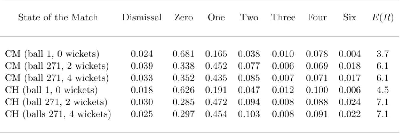
Now, there are countless ways that one might test the adequacy of the model. In Table 2.3, we provide the estimated probabilities pijwbk for some batsmen/bowler combinations at different states of a match. We have also included the expected number of runs per over for each combination. We have presented batting outcome probabilities when Alistair Cook of England is batting against Glenn McGrath of Australia, and against Nazmul Hossain of Bangladesh. At the beginning of a match (i.e. ball 1, 0 wickets), we observe that with probabilities 0.681 and 0.078, Cook scores 0 runs and 4 runs respectively against McGrath. At the beginning of a match, these probabilities change to 0.626 and 0.100 respectively when Hossain is bowling. These changes are consistent with the general belief that McGrath is a better bowler than Hossain. We then investigate a situation where batsmen ought to become more aggressive (ball 271 when 2 wickets are lost). Indeed, the probability that Cook scores 0 runs decreases substantially to 0.338 and 0.285 depending on whether McGrath or Hossain is the bowler. We also note a curious result concerning the probability of scoring 4 runs. Even though batsmen are more aggressive on ball 271 with 2 wickets than at the beginning of a match (ball 1 with 0 wickets), the fielding restriction that is in place at the beginning of a match enables batsmen to score 4’s at a higher rate. This batting behaviour is observed in Table 2.3 and has been verified by looking at empirical data. In Table 2.3, we also investigate the case of ball 271 when 4 wickets are lost which according to common knowledge should be a less aggressive batting situation than ball 271 when 2 wickets are lost. Accordingly, we observe that the probability of 0s increase and the probability of 1s decrease in the less aggressive situation.
Table 2.3: Batting probabilitiespfor various states and the expected number of runs per over E(R) where CM denotes the Cook/McGrath matchup and CH denotes the Cook/Hossain matchup.
State of the Match Dismissal Zero One Two Three Four Six E(R)
CM (ball 1, 0 wickets) 0.024 0.681 0.165 0.038 0.010 0.078 0.004 3.7 CM (ball 271, 2 wickets) 0.039 0.338 0.452 0.077 0.006 0.069 0.018 6.1 CM (ball 271, 4 wickets) 0.033 0.352 0.435 0.085 0.007 0.071 0.017 6.1 CH (ball 1, 0 wickets) 0.018 0.626 0.191 0.047 0.012 0.100 0.006 4.5 CH (ball 271, 2 wickets) 0.030 0.285 0.472 0.094 0.008 0.088 0.024 7.1 CH (balls 271, 4 wickets) 0.025 0.297 0.454 0.103 0.008 0.091 0.022 7.1
again the matchup between the batsman Cook and the bowler Hossain. Suppose that Bangladesh has scoredf = 250 runs in the first innings. Suppose further that ballb= 183 is about to be bowled and w = 3 wickets have been lost in the second innings (situation 2). From the Duckworth/Lewis table, we therefore have the proportion of resources lost x = 0.0027 due to the current ball and the proportion of resources lost y = 0.044 due to a wicket. This might be considered as a “middle point” of the second innings since the proportion of resources used is R(w, b) = 0.4993, and therefore, the proportion of resources remaining is r = 0.5007. In this case, the estimated parameters give E1(p) = 0.9723 and
E2(p) = 0.00393. We now investigate the outcome probabilities p0ijwbk when England has
scoreds= 127,90,60 runs. Whens= 127, then (f−s+1)/r= 247.7≈E1(p)/E2(p) = 247.5
and England is on pace to draw the match, and p0 =p (i.e. no adjustment). When s= 90, Cook should become more aggressive (c = 0.768), and when s= 60, Cook should become even more aggressive (c= 0.648). The entries in Table 2.4 appear reasonable and support these tendencies.
We now compare actual runs versus simulated runs. For this, we consider the 23 matches between Sri Lanka and India from November 1998 through March 2007 in which Sri Lanka batted first. The 23 matches consist of 15 matches from the original dataset (2001-2006)
Table 2.4: Second innings batting probabilities p0 and the expected number of runs per over for the Cook/Hossain matchup when Bangladesh has scored f = 250 runs in the first innings. In the second innings, w = 3 wickets have been lost, ballb = 183 is about to be bowled and England has scoredsruns.
England Runs (s) Dismissal Zero One Two Three Four Six Runs/Over
127 0.016 0.452 0.397 0.058 0.008 0.062 0.008 5.0 90 0.029 0.347 0.466 0.068 0.010 0.072 0.009 5.8 60 0.036 0.293 0.501 0.073 0.010 0.078 0.010 6.3
used for model fitting and 8 matches outside of the training period. We simulate 1000 first innings results for Sri Lanka based on representative batting and bowling orders employed during the time period. The resultant QQ plot comparing the actual runs and the simulated runs is given in Figure 2.2. We observe excellent agreement and we remark that satisfactory plots are also observed for other pairs of teams that we investigated. In comparing wickets taken, the actual results also compare favourably with the simulated results.
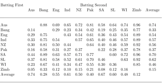
We also investigate the effect of the second innings adjustment. The difficulty in this exercise is that given the number of first innings runs between two teams, replicate observa-tions tend not to occur. Therefore, to address goodness-of-fit, we provide some evidence that the second innings adjustment p0 is an improvement over having the second innings team bat in a neutral fashion (i.e. p0 =p). Consider then simulated matches between Australia and the other 9 ICC teams where Australia is batting in the second innings and where the batting and bowling lineups resemble those used in the 2007 World Cup matches. We gen-erate first innings runs for the other teams, and then second innings runs for Australia with the proposed batting adjustment p0 based on the target scores. The simulation is repeated for 1000 hypothetical matches for each of the 9 teams. We observe that Australia uses their full 50 overs in 8.5% of the simulated matches. The small percentage seems sensible since Australia rarely uses all 50 overs in matches that they win. In matches that Australia
• • • • • • • • • • • • • • • • • • • • • • • simulated runs actual runs 150 200 250 300 150 200 250 300
Figure 2.2: QQ plot corresponding to first innings runs for Sri Lanka batting against India. loses, at some point when they are falling behind, they become desperate (aggressive), and typically consume all of their wickets before using the allotted 50 overs. When we repeat the simulation with neutral batting in the second innings (i.e. Australia behave as they would in the first innings), Australia uses all 50 overs 13% of the time. To get a sense of the percentages using actual data, we look at all 83 matches from 2000 to 2006 where Australia batted second, and observe that Australia used the full 50 overs only 7% of the time. This suggests that there is merit in our modification of aggressiveness in second innings batting.
2.6
Addressing questions via simulation
Having developed a simulator for ODI cricket matches, there is no limit to the number and type of questions that may be posed. The greatest utility of the simulator occurs for circumstances in which there is limited empirical data. In these cases, without a simulator, the best that one can do is to rely on hunches with respect to the questions of interest. In this section, we give a flavour for the types of questions that might be posed. We see these
types of applications as being of value not only to cricket devotees but also to selection committees and team strategists. We note that each of the simulations described below requires less than one minute of computation.
2.6.1 Question 1.
Adam Gilchrist is often an opening batsman for Australia, and Australia has not played the West Indies often in recent history. We are interested in the probability of Gilchrist hitting a century as an opening batsman against the West Indies when Australia is batting in the first innings and the West Indies are using a bowlng lineup from the 2007 World Cup. Based on 1000 first innings simulations, Gilchrist reaches a century 5.1% of the time. The result appears consistent with Gilchrist’s actual batting performances where Gilchrist made a century 8 times as an opening batsman in 138 first innings ODI matches (5.8%) throughout his career (1996-2008).
2.6.2 Question 2.
England has occasionally sent Alastair Cook and Matt Prior as opening batsmen. In other matches, they used Ian Bell and Michael Vaughan as opening batsmen. We are interested in the performance in the untested opening partnership of Alastair Cook and Ian Bell. More specifically, we consider the length of the partnership (i.e. the number of overs prior to losing the first wicket) for Cook and Bell when they are batting in the first innings against Pakistan where Pakistan uses a bowling lineup comparable to the lineup used in their December 15/2005 match against England. In Figure 2.3, we provide a histogram of the number of overs in the length of their partnership based on 1000 simulations. We observe that the median and the mean length of the partnership is 5 overs and 7.1 overs respectively. It appears very unlikely for Cook and Bell to have a partnership exceeding 20 overs.
2.6.3 Question 3.
Consider a match between New Zealand and Sri Lanka where Sri Lanka is batting in the second innings and New Zealand has scored an impressive 300 runs in the first innings.