llll
1
-Penalised quantile
regression in
high-dimensional sparse models
Alexandre Belloni
Victor Chernozhukov
The Institute for Fiscal Studies
Department of Economics, UCL
cemmap working paper CWP10/09SPARSE MODELS
By Alexandre Belloni and Victor Chernozhukov∗,†
Duke University and Massachusetts Institute of Technology We consider median regression and, more generally, quantile re-gression in high-dimensional sparse models. In these models the over-all number of regressorspis very large, possibly larger than the sam-ple sizen, but onlysof these regressors have non-zero impact on the conditional quantile of the response variable, where s grows slower thann. Since in this case the ordinary quantile regression is not con-sistent, we consider quantile regression penalized by the`1-norm of coefficients (`1-QR). First, we show that `1-QR is consistent at the rateps/n√logp, which is close to the oracle rateps/n, achievable when the minimal true model is known. The overall number of re-gressorspaffects the rate only through the logpfactor, thus allowing nearly exponential growth in the number of zero-impact regressors. The rate result holds under relatively weak conditions, requiring that s/nconverges to zero at a super-logarithmic speed and that regular-ization parameter satisfies certain theoretical constraints. Second, we propose a pivotal, data-driven choice of the regularization parame-ter and show that it satisfies these theoretical constraints. Third, we show that`1-QR correctly selects the true minimal model as a valid submodel, when the non-zero coefficients of the true model are well separated from zero. We also show that the number of non-zero co-efficients in `1-QR is of same stochastic order as s, the number of non-zero coefficients in the minimal true model. Fourth, we analyze the rate of convergence of a two-step estimator that applies ordi-nary quantile regression to the selected model. Fifth, we evaluate the performance of`1-QR in a Monte-Carlo experiment, and provide an application to the analysis of the international economic growth.
∗First version: December, 2007, This version: April 19, 2009.
†The authors gratefully acknowledge the research support from the National Science Foundation.
AMS 2000 subject classifications:Primary 62H12, 62J99; secondary 62J07
Keywords and phrases:median regression, quantile regression, sparse models
1. Introduction. Quantile regression is an important statistical method for analyzing the impact of regressors on the conditional distribution of a response variable (cf. Laplace [22], Koenker and Bassett [20]). In particular, it captures the heterogeneity of the impact of regressors on the different parts of the distribution [7], exhibits robustness to outliers [19], has excellent computational properties [29], and has a wide applicability [19]. The asymptotic theory for quantile regression is well-developed under both fixed number of regressors and increasing number of regressors. The asymptotic theory under fixed number of regressors is given by Koenker and Bassett [20], Portnoy [28], Gutenbrunner and Jureˇckov´a [14], Knight [17], Chernozhukov [9] and others. The asymptotic theory under increasing number of regressors is given in He and Shao [15] and Belloni and Chernozhukov [4, 5], covering the case where the number of regressorsp is negligible relative to the sample size
n(p=o(n)).
In this paper, we consider quantile regression in high-dimensional sparse models (HDSMs). In such models, the overall number of regressorsp is very large, possibly much larger than the sample sizen. However, the numbersof significant regressors – those having a non-zero impact on the response variable – is smaller than the sample size, that is,s = o(n). The HDSMs ([8], [26]) have emerged to deal with many new applications, arising in biometrics, signal processing, machine learning, econometrics, and other areas of data analysis, where high-dimensional data sets have become widely available.
A number of papers began to investigate estimation of HDSMs, primarily focusing on penalized mean regression, with`1-norm acting as a penalty function. Candes and Tao [8]
demonstrated that, remarkably, an estimator, called the Dantzig selector, achieves the rate p
s/n√logp, which is very close to the oracle rate ps/n obtainable when the significant regressors are known. Thus the estimator can be consistent even under very rapid, nearly exponential growth in the total number of regressorsp. Meinshausen and Yu [26] and Zhang and Huang [39] demonstrated similar striking results for the `1-penalized least squares
proposed by Tibshirani [35]. van der Geer [37] derived valuable finite sample bounds on empirical risk for`1-penalized estimators in generalized linear models. Fan and Lv [11] used
screening and derived asymptotic results under even weaker conditions on p. There were many other interesting developments, which we shall not review here.
Our paper’s contribution is to develop, within the HDSM framework, a set of results on model selection and rates of convergence for quantile regression. Since ordinary quantile regression is not consistent in HDSMs, we consider quantile regression penalized by the
consistent at the rateps/n√logp, which is close to the oracle rateps/nachievable when the true minimal model is known. In order to make the penalized estimator practical, we propose a pivotal, data-driven choice of the regularization parameter, and show that this choice leads to the same sharp convergence rate. Further, we show that the penalized quantile regression correctly selects the true minimal model as a valid submodel, when the non-zero coefficients of the true model are well separated from zero. We also analyze a two-step estimator that applies standard quantile regression to the selected model and aims at reducing the bias of the penalized quantile estimator. We illustrate the use of the penalized and post-penalized estimators with a Monte carlo experiment and an international economic growth example. Thus, our results contribute to the literature on HDSMs by examining a new class of problems. Moreover, our proof strategy, developed to cope with non-linearities and non-smoothness of quantile regression, may be of interest in other M-estimation problems. (We provide more detailed comparisons to the literature in Section
2.)
Finally, let us comment on the role of computational considerations in our analysis. The choice of the`1-penalty function arises from considering a tradeoff between statistical
efficiency and computational efficiency, with the latter being of particular importance in high-dimensional applications. Indeed, in model selection problems, the statistical efficiency criterion favors the use of the`0-penalty functions (Akaike [1] and Schwarz [32]), where the `0-penalty counts the the number of non-zero components of a parameter vector. However, the computational efficiency criterion favors the use of convex penalty functions. Indeed, convex penalty functions lead to efficient convex programming problems ([27]); in contrast, the `0-penalty functions lead to inefficient combinatorial search problems, plagued by the
computational curse of dimensionality. Precisely because it is a convex function that is closest to the `0-penalty (e.g. [30]), the `1-penalty has emerged to play a central role in HDSMs, in general (e.g. [25]), and in our analysis, in particular. In other words, the use of the `1-penalty takes us close to performing the most effective model selection, while
respecting the computational efficiency constraint.
We organize the rest of the paper as follows. In Section2, we introduce the problem and some simple primitive assumptions D.1-D.4, and propose pivotal choices for the regular-ization parameter. We also describe our key results under D.1-D.4, and provide detailed comparisons with the literature. In Section 3, we develop the main results under condi-tions E.1-E.5, which are implied by D.1-D.4, and also hold much more generally. Section4
com-putational experiment and provide an application to an international growth example. In Section6, we provide conclusions and discuss possible extensions. In AppendixA, we verify that conditions E.1-E.5 are implied by conditions D.1-D.4 and also hold more generally.
1.1. Notation. In what follows, we implicitly index all parameter values by the sample
sizen, but we omit the index whenever this does not cause confusion. We carry out all of the asymptotic analysis asn→ ∞. We use the notationa.bto denote thata=O(b), that isa≤cbfor all sufficiently largen, for some constantc >0 that does not depend onn, and we use a.p b to denote thata =Op(b); we use a' b to denotea .b. aand a'p b to denotea.p b.p a. We also use the notation a∨b= max{a, b} and a∧b= min{a, b}. We denote`2-norm by k · k,`1-norm by k · k1,`∞-norm by k · k∞, and the `0-“norm” byk · k0.
2. Basic Settings, the Estimator, and Overview of Results. In this section, we formulate the setting, the estimator, and state primitive regularity conditions. We also provide an overview of the main results.
2.1. Basic Setting. The set-up of interest corresponds to a parametric quantile regression
model, where the dimension p of the underlying model increases with the sample size n. Namely, we consider a response variable y and p-dimensional covariates x such that the
u-th conditional quantile function ofy given x is given by
(2.1) Qy|x(u) =x0β(u), β(u)∈IRp.
We consider the case where the dimensionpof the model is large, possibly much larger than the available sample size n, but the true model β(u) is sparse having only s = s(u) < p
non-zero components. Throughout the paper the quantile indexu∈(0,1) is fixed. The population coefficientβ(u) is known to be a minimizer of the criterion function
Qu(β) = E[ρu(y−x0β)], (2.2)
where ρu(t) = (u−1{t ≤ 0})t is the asymmetric absolute deviation function [20]. Given a random sample (y1, x1), . . . ,(yn, xn), the quantile regression estimator βb(u) of β(u) is defined as a minimizer of
(2.3) Qbu(β) =En
£
ρu(yi−x0iβ) ¤
whereEn[f(yi, xi)] :=n−1Pni=1f(yi, xi) denotes the empirical expectation of a function f in the given sample.
In the high-dimensional settings, particularly whenp≥n, quantile regression is generally not consistent, which motivates the use of penalization in order to remove all or at least nearly all regressors whose population coefficients are zero, thereby possibly restoring con-sistency. The penalization that has been proven to be quite useful in least squares settings is the`1-penalty leading to the lasso estimator [35].
2.2. The Choice of Estimator, Linear Programming Formulation, and Its Dual. The
`1-penalized quantile regression estimator βb(u) is a solution to the following optimization
problem: (2.4) min β∈Rp b Qu(β) +λ n p X j=1 |βj|.
When the solution is not unique, we define βb(u) as a basic solution having the minimal number of non-zero components. The criterion function in (2.4) is the sum of the criterion function (2.3) and a penalty function given by a scaled `1-norm of the parameter vector.
This `1-penalized quantile regression or quantile regression lasso has been considered by
Knight and Fu [18] under the small (fixed) p asymptotics.
For computational purposes, it is important to note that the penalized quantile regression problem (2.4) is equivalent to the following linear programming problem
(2.5) ξ+,ξ−,β+min,β−∈R2n+2p + Enhuξ+i + (1−u)ξi−i+λ n p X j=1 (βj++βj−) ξi+−ξ−i =yi−x0i(β+−β−), i= 1, . . . , n.
The problem minimizes a sum of`1-norm of the absolute positiveβj+and negativeβj−parts
of the parameter βj = βj+−βj− and of an average of asymmetrically weighted residuals
ξi+ and ξi−. The linear programming formulation (2.5) is useful for computation of the estimator, particularly in high-dimensional applications. There are a number of efficient, that is, polynomial time, algorithms for the linear programming problem (2.5). Using these algorithms, one can compute the estimator (2.4) efficiently, avoiding the computational curse of dimensionality.
Furthermore, for both computational and theoretical purposes, it is important to note that the primal problem (2.5) has the following dual problem:
(2.6)
max
a∈Rn En[yiai]
|En[xijai]| ≤ nλ, j= 1, . . . , p, (u−1)≤ai≤u, i= 1, . . . , n.
The dual problem maximizes the correlation between the response variable and the rank scores subject to the condition requiring the rank scores to be approximately uncorrelated with the regressors. This condition is reasonable, since the true rank scores, defined as
a∗
i(u) = (u−1{yi ≤x0iβ(u)}), should be independent of regressorsxi. This follows because by (2.1) the event{yi≤x0iβ(u)}is equivalent to the event{ui ≤u}, for a standard uniformly distributed variableui which is independent ofxi.
Since both primal and dual problems are feasible, by strong duality for linear program-ming the optimal values of (2.6) equals the optimal value of (2.4) (see, for example, Bert-simas and Tsitsiklis [6]). The optimal solution to the dual problem plays an important role in our analysis, helping us control the sparseness of the penalized estimator βb(u) as well as choose the penalization parameter λ. Of course, the optimal solution to the dual prob-lem (2.6) also plays an important role in the non-penalized case, with λ= 0, yielding the regression generalization of Hajek-Sidak rank scores (Gutenbrunner and Jureˇckov´a [14]).
Another potential approach worth considering is the Dantzig selector approach of Candes and Tao [8], proposed in the context of mean regression. We can extend this approach to quantile regression by defining the estimator as solution to the following problem:
(2.7) inf β∈Rp p X j=1 |βj|: kSbu(β)k∞≤ γn,
where λ is a penalization parameter, and Sbu is a subgradient of the quantile regression objective functionQbu(β):
(2.8) Sbu(β) =En[(1{yi ≤x0iβ} −u)xi].
The estimator (2.7) minimizes the `1-norm of the coefficients subject to a goodness-of-fit
constraint.
On computational grounds, we prefer the`1-penalized estimator (2.4) over to the Dantzig selector estimator (2.7). The reason is that the subgradientSbu in (2.8) is a piece-wise con-stant function in parameters, leading to a serious difficulty in computing the estimator (2.7). In particular, the problem (2.7) can be recast as a mixed integer programming prob-lem withnbinary variables, for which (generally) there is no known polynomial time algo-rithm. (In sharp contrast, in the mean regression case the subgradient is a linear function,
b
S(β) =En[(yi−xiβ)xi], corresponding to the objective function Qb(β) =En[(yi−xiβ)2]/2. Accordingly, in the mean regression case, the optimization problem can be recast as a linear programming problem, for which there are polynomial time algorithms.)
Another idea for formulating a Dantzig type estimator for quantile regression would be to minimize the `1 norm of the coefficients subject to a convex goodness-of-fit constraint,
namely (2.9) min β∈Rp p X j=1 |βj| :Qbu(β)≤γ.
Since the constraint set {β :Qbu(β) ≤γ} is piece-wise linear and convex, this problem is equivalent to a linear programming problem. Of course, this is hardly a surprise, since this problem is equivalent to an`1-penalized quantile regression problem (2.4) that we started
with in the first place. Indeed, for every feasible choice ofγ in (2.9) there is a feasible choice of λthat makes the solutions to (2.9) and to (2.4) identical. To see this, fix a γ and let κ
denote the optimal value of the Lagrange multiplier for the constraintQbu(β)≤γ, then the problem (2.9) is equivalent to minβ∈Rp Ppj=1|βj|+κ(Qbu(β)−γ),which is then equivalent
to the original problem (2.4) withλ = n/κ. Therefore it suffices to focus our analysis on the original problem.
2.3. The Choice of the Regularization Parameter. Here we propose a pivotal, data-driven
choice for the regularization parameter value λ. We shall verify in Section 4 that such choice will agree with our theoretical choice of λ maximizing the speed of convergence of the penalized estimate to the true parameter value.
Because the objective function in the primal problem (2.4) is not pivotal in either small or large samples, finding a pivotalλappears to be difficult a priori. However, instead of looking at the primal problem, let us look at its linear programming dual (2.6), which requires that (2.10) |En[xijai]| ≤
λ
n,for all j= 1, . . . , p⇔ kEn[xiai]k∞≤ λ n.
This restriction requires that potential rank scores must be approximately uncorrelated with regressors. It then makes sense to selectλso that the true rank scores
a∗i(u) = (u−1{yi≤x0iβ(u)}) for i= 1, . . . , n satisfy this constraint. That is, we can potentially setλ= Λn, where
(2.11) Λn=nkEn[xia∗i(u)]k∞.
Of course, since we do not observe the true rank scores, this choice is not available to us. The key observation is that the finite sample distribution of Λn is pivotal conditional on
the regressorsx1, . . . , xn. We know that rank scores can be represented almost surely as
a∗i(u) = (u−1{ui ≤u}), fori= 1, . . . , n,
whereu1, . . . , un are i.i.d. uniform (0,1) random variables, independently distributed from the regressors,x1, . . . , xn. Thus, we have
(2.12) Λn=nkEn[xi(u−1{ui ≤u})]k∞,
which has a known distribution conditional on x1, . . . , xn. Therefore we can use the tail quantiles Λn as our choice for λ. In particular, we set λ = λ(x1, . . . , xn) as the 1−αn quantile of Λn
(2.13) λ= inf{c:P(Λn≤c|x1, . . . , xn)≥1−αn}, whereαn&0 at some rate to be determined below.
Finally, let us note that we can also derive the pivotal quantity Λn, and thus also our choice of the regularization parameterλ, from the subgradient characterization of optimality for the primal problem (2.4).
2.4. Primitive Conditions. We follow Huber’s framework of high-dimensional
parame-ters [16], which formally consists of a sequence of models with parameter dimensionp=pn
tending to infinity as the sample sizengrows to infinity. Thus, the parameters of the mod-els, the parameter space, and the parameter dimension are all indexed by the sample size
n. However, following Huber’s convention, we will omit the indexnwhenever this does not cause confusion. Let us consider the following set of conditions:
D.1. Sampling. Data (yi, x0i)0, i = 1, . . . , n are an i.i.d. sequence of real (1 +p)-vectors, with the conditionalu-quantile function given by (2.1), and with the first component ofxi equal to one.
D.2. Sparseness of the True Model. The number of non-zero components of β(u) is
bounded by 1≤s=sn≤n/log(n∨p).
D.3. Smooth Conditional Density. The conditional densityfyi|xi(y|x) and its derivative ∂
∂yfyi|xi(y|x) are bounded above uniformly in y and x ranging over supports of yi and xi,
and uniformly inn.
D.4. Identifiability in Population and Well-Behaved Regressors.Eigenvalues of the
is bounded above, uniformly inn. The conditional density evaluated at the conditional quan-tile,fyi|xi(x0β(u)|x) is bounded away from zero, uniformly inx ranging over the support of
xi, and uniformly in n.
The conditions D.1-D.4 stated above are a set of simple conditions that ensure that the high-level conditions developed in Section3hold. These conditions allow us to demonstrate the general applicability of our results and straightforwardly compare to other results in the literature. In particular, condition D.1 imposes random sampling on the data, which is a conventional assumption in asymptotic statistics (e.g [38]). Condition D.2 requires that the effective dimension of the true model is smaller than the sample size. Condition D.3 imposes some smoothness on the conditional distribution of the response variable. Condition D.4 requires the population design matrix to be uniformly non-singular and the regressors’ moments to be well-behaved.
Further, let φ(k) be the maximal k-sparse eigenvalue of the empirical design matrix
En[xix0 i], that is, (2.14) φ(k) = sup kαk≤1,kαk0≤k En h (α0xi)2 i .
Following Meinshausen and Yu [26], we will state our general results on convergence rates of the penalized estimator in terms of the maximal sparse eigenvalueφ(m0). Meinshausen and
Yu [26] worked withm0 =n∧pas an initial upper bound on the zero norm of the penalized estimator. In this paper we can work with a smaller m0, in particular, under D.1-D.4, we
can work with
m0 =p∧(n/log(n∨p)),
as this provides a valid initial bound on the zero norm of our penalized estimator under a suitable choice of the penalization parameter.
By using an assumption on the growth rate ofφ(k), we avoid imposing Candes and Tao’s [8] uniform uncertainty principle on the empirical design matrixEn[xix0i]. Meinshausen and Yu [26] argue that the assumption in terms of φ(k) are less stringent than the uniform uncertainty principle, since it allows for non-vanishing correlation between the regressors. Meinshausen and Yu [26] provide a thorough discussion of the behavior of φ(n) in many cases of interest. In particular, they show that the conditionφ(n).p 1 appears reasonable in several cases (for example, when the empirical design matrix is block diagonal). Note that if the intercept is included as a covariate we haveφ(1)≥1. For the purposes of a basic
overview of results in the next subsection, we employ the assumption
(2.15) φ(n/log(n∨p)).p1.
which will cover standard Gaussian regressors and some other regressors considered in Meinshausen and Yu [26] (because φ(n/log(n∨p))≤ φ(n)). Furthermore, in our general analysis presented in Section3, we do not impose (2.15) and allow for the sparse eigenvalue
φ(n/log(n∨p)) to diverge, which should permit for situations with regressors having tails thicker than Gaussian.
In order to illustrate our conditions we employ the following canonical examples through-out the paper.
Example 1 (Isotropic Normal Design). Let us consider estimating the median (u = 1/2) of the following regression model
y =x0β0+ε,
where the covariatex1= 1 is the intercept and the covariatesx−1 ∼N(0, I), and the errors are independent identically distributed with a smooth probability density function which is positive at zero and has bounded derivatives. This example satisfies conditions D.1, D.3, D.4, and D.2 ifkβ0k0 ≤ s=o(n/log(n∨p)). Moreover, the maximal k-sparse eigenvalues
fork≤n satisfy φ(k) := sup kαk=1,kαk0≤k En h (α0xi)2 i 'p 1 + s klogp n
by Lemma14. Thus, this design satisfies our conditions withφ(n/log(n∨p))'p 1. Moreover, as shown in [8], this design satisfies Candes and Tao’s uniform uncertainty principle.
Example 2 (Correlated Normal Design). We consider the same setup as in Example
1, but instead we suppose that the covariates are correlated, namelyx−1 ∼N(0,Σ), where
Σij =ρ|i−j| and −1 < ρ <1 is fixed. This example satisfies conditions D.1, D.3, D.4, and D.2 ifkβ0k0 ≤s=o(n/log(n∨p)). The maximalk-sparse eigenvalues for k≤nsatisfy
φ(k) := sup kαk=1,kαk0≤k En h (α0xi)2 i 'p 1 +1− ||ρρ|| 1 + s klogp n
by Lemmas14. Thus, this design satisfies our conditions withφ(n/log(n∨p))'p 1. However, as mentioned in [26] this design violates Candes and Tao’s uniform uncertainty principle, which requires|ρ| →0 at logp rate.
Finally, it is worth noting that our analysis in Sections3and4, and in AppendixAallows the key parameters of the model, such as the bounds on the eigenvalues of the design matrix and on the density function, to change with the sample size. This will explicitly allow us to trace out the impact of these parameters on the large sample behavior of the penalized estimator. In particular, we will be able to immediately see how some basic changes in the primitive conditions stated above affect the large sample behavior of the penalized estimator.
2.5. Overview of Main Results. Here we discuss our results under simplest assumptions,
consisting of conditions D.1-D.4 and condition (2.15) on the maximal (n/log(n∨p))-sparse eigenvalue. These simplest assumptions allow us to straightforwardly compare our results to those obtained in the literature, without getting into nuisance details. We state our results under more general conditions in the subsequent sections: in Section 3, we present various results on convergence rates and model selection; in Section 4, we analyze our choice of the penalization parameter.
In order to achieve the most rapid rate of convergence, we need to choose
(2.16) λ=t
q
nlog(n∨p)
withtgrowing as slowly as possible with n; for concreteness, lett∝log logn.
Our first main result is that the `1-penalized quantile regression estimator converges at
the rate: (2.17) kβb(u)−β(u)k.p λ √ s n = r s n·t· q log(n∨p),
provided that the number of non-zero componentsssatisfies (2.18) r s n·t· q log(n∨p)→0.
We note that the total number of regressors p affects the rate of convergence (2.17) only through a logarithm inp. Hence ifp is polynomial in n, the rate of convergence is ps/n·
t·plog(n∨p), which is very close to the oracle rate ps/n, obtainable when we know the minimal true model. Further, we note that our resulting restriction (2.18) on the dimension
s of the minimal true model is very weak; whenp is polynomial in n and t ∝ log logn, s
can be of almost the same order asn, namely s=o(n/(t2logn))).
Our second main result is that the dimensionkβb(u)k0 of the model selected by the `1
model, namely
(2.19) kβb(u)k0.p s.
Further, if the parameter values of the minimal true model are well separated away from zero, namely (2.20) min j∈support(β(u))|βj(u)|> `· r s n·t· q log(n∨p),
for some diverging sequence`of positive constants, then with probability converging to one, the model selected by the`1-penalized estimator correctly nests the true minimal model:
(2.21) support (β(u))⊆support (βb(u)).
Moreover, we provide conditions under which a hard-thresholding selects the correct sup-port.
Our third main result is that a two-step estimator, which applies standard quantile re-gression to the selected model, achieves a similar rate of convergence:
(2.22) r s n q log(n∨p)→0,
provided the true non-zero coefficients are well-separated from zero in the sense of equation (2.20).
Finally, our fourth main result is to propose (2.13), a data-driven choice of the regu-larization parameter λ which has a pivotal finite sample distribution conditional on the regressors, and to verify that (2.13) satisfies the theoretical restriction (2.16), supporting its use in practical estimation.
Our results for quantile regression parallel the results for least squares by Meinshausen and Yu [26] and by Candes and Tao [8]. Our results on the pivotal choice of the regularization parameter partly parallel the results by Candes and Tao [8], except that our choice is pivotal whereas Candes and Tao’s choice relies upon the knowledge of the standard deviation of the regression disturbances. The existence of close parallels may seem surprising, since, in contrast to the least squares problem, our problem is highly non-linear and non-smooth. Nevertheless, there is an intuition presented below, suggesting that we can overcome these difficulties.
While our results for quantile regression parallel results for least squares, our proof strat-egy is substantially different, as it has to address non-linearities and non-smoothness. In
order to explain the difference, let us recall, e.g., the proof strategy of Meinshausen and Yu [26]. They first analyze the problem with no disturbances, recognize sparseness of the solution for this zero noise problem, and then analyze a sequence of problems along the path interpolating the zero-noise problem and the full-noise problem. Along this sequence, they bound the increments in the number of non-zero components and in the rates of convergence. This approach does not seem to work for our problem, where the zero-noise problem does not seem to have either the required sparseness or the required smoothness. In sharp contrast, our approach directly focuses on the full-noise problem, and simultaneously bounds the number of non-zero components and convergence rates. Thus, our approach may be of independent interest for other M-estimation problems and even for the least squares problem.
Our analysis is perhaps closer in spirit to, but still quite different from, the important work of van der Geer [37] which derived finite sample bounds on the empirical risk of `1
-penalized estimators in generalized linear models (but did not investigate quantile regression models). The major difference between our proof and van der Geer [37]’s proof strategies is that we analyze the sparseness of the solution to the penalized problem and then further exploit sparseness to control empirical errors in the sample criterion function. As a result, we derive not only the results on model selection and on sparseness of solutions, which are of a prime interest, but also the results on the consistency and rates of convergence under weak conditions on the number of non-zero components s. As mentioned above, our approach allows s to be of almost the same order as the sample size n, and delivers convergence rates that are close to ps/n. In contrast, van der Geer’s [37] approach requires s to be much smaller than n, namely s2/n → 0, and thus does not deliver consistency or rates of convergence whens2/n→ ∞.
In our proofs we critically rely on two key quantities: the number of non-zero components
m=kβb(u)k0 of the solution βb(u) and the empirical error in the sample criterion,Qbu(β)−
Qu(β) (withβranging over allm-dimensional submodels of the largep-dimensional model). In particular, we make use of the following relations:
(1) lowermimplies smaller empirical error, and (2) smaller empirical error can imply lowerm.
Starting with a structural initial upper bound onm (see condition E.3 below) we can use the two relations to solve for sharp bounds on m and the empirical error, given which we then can solve for convergence rates.
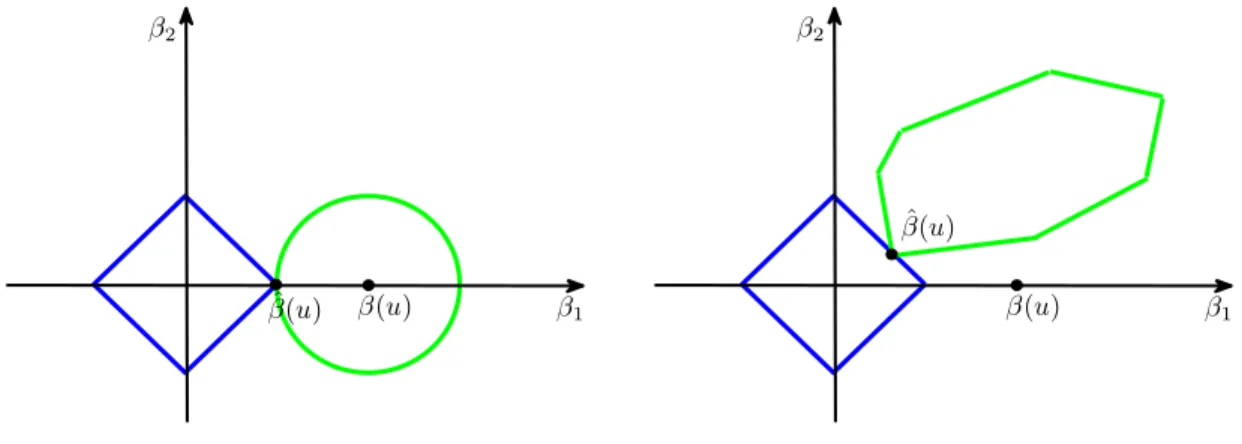
an application of the usual entropy-based maximal inequalities, upon realizing that the en-tropy of allm dimensional models grows at the ratemlogp. In particular, the lower them, the closer the sample criterion functionQbu to a locally quadratic function, uniformly across all m-dimensional submodels. Relation (2) follows from the use of`1-penalty, which tends to favor lower-dimensional solutions whenQbu is close to being quadratic. Figure 1 provides a visual illustration of this, using a two-dimensional example with a one-dimensional true minimal submodel; in the example, the true parameter value (β1(u), β2(u)) is (1,0).
Fig-ure1 plots a diamond, centered at the origin, representing a contour set of the `1-penalty
function and a pearl, representing a contour set of the criterion functionQbu. By the dual interpretation (2.9) of our estimation problem, the penalized estimator looks for a minimal diamond, subject to the diamond having a non-empty intersection with a fixed pearl. The set of optimal solutions is then given by the intersection of the minimal diamond with the pearl. Smaller empirical errors shape the pearl into an ellipse and center it closer to the true parameter value of (1,0) (left panel of Figure 1). Larger empirical errors shape the pearl like a non-ellipse and can center it far away from the true parameter value (right panel of Figure 1). Therefore, smaller empirical errors tend to cause sparse optimal solutions, cor-rectly settingβb2(u) = 0; larger empirical errors tend to cause non-sparse optimal solutions,
incorrectly settingβb2(u)6= 0. β1 β2 ˆ β(u) β(u) β1 β2 β(u) ˆ β(u)
Fig 1. These figures provide a geometric illustration for the discussion given in the text concerning why
`1-penalized estimation may be (left panel) or may not be (right panel) successful at selecting the minimal
true model.
3. Analysis and Main Results Under High-Level Conditions. In this section we prove the main results under general conditions that encompass the simple conditions
D.1-D.4 as a special case.
3.1. The Five Basic Conditions. We will work with the following five basic conditions
E.1-E.5 which are the essential ingredients needed for our asymptotic approximations. In AppendixA, we verify that conditions E.1-E.5 hold under simple sufficient conditions D.1-D.4 stated in Section 2, and we also show that E.1-E.5 arise much more generally. In particular, in Appendix A we characterize key constants appearing in E.1-E.5 in terms of the parameters of the model.
E.1. True Model Sparseness.The true parameter valueβ(u) has at most s < n/log(n∨p)
non-zero components, namely
(3.1) kβ(u)k0 =s < n/log(n∨p).
E.2. Identification in Population.In the population, the true parameter value β(u) is the
unique solution to the quantile objective function. Moreover, the following minorization condition holds,
(3.2) Qu(β)−Qu(β(u))&q ³
kβ−β(u)k2∧g(kβ−β(u)k)´,
uniformly in β ∈ IRp, where g :R+ → R+ is a fixed convex function with g0(0)> 0, and q is a sequence of positive numbers that characterizes the strength of identification in the population.
E.3. Empirical Pre-Sparseness.The number m=kβb(u)k0 of non-zero components of βb(u)
of the solution to the penalized quantile regression problem (2.4) obeys the inequality
(3.3) m≤n∧p∧ n2φ(m)
λ2 ,
whereφ(m) is the maximal m-sparse eigenvalue.
E.4. Empirical Sparseness.Forr=kβb(u)−β(u)k,m=kβb(u)k0obeys the following
stochas-tic inequality (3.4) √m.pµn λ(r∧1) + √ m p nlog(n∨p)φ(m) λ ,
whereµ≥q is a sequence of positive constants. The sequence of constantsµis determined by the population analog of the empirical sparse eigenvalueφ(m0) (cf. Appendix A).
E.5. Sparse Control of Empirical Error. The empirical error that describes the deviation
inequality
(3.5) ¯¯¯ bQu(β)−Qu(β)−³Qbu(β(u))−Qu(β(u))´¯¯¯.p r
s
(m+s) log(n∨p)φ(m+s)
n ,
uniformly over{β ∈IRp :kβk0 ≤m∧n∧p, kβ−β(u)k ≤r},uniformly overm≤n, r ≥0.
Let us briefly comment on each of the conditions. As stated earlier, condition E.1 is a basic modeling assumption, and condition E.2 is an identification assumption, required to hold in population. Conditions E.3 and E.4 arise from two characterizations of sparseness of the solution to the optimization problem (2.4) defining the estimator. Condition E.3 arises from simple bounds applied to the first characterization. Condition E.4 arises from maxi-mal inequalities applied to the second characterization. Condition E.5 arises from maximaxi-mal inequalities applied to the empirical criterion function. To derive conditions E.4 and E.5, we crucially exploit the fact that the entropy of all m-dimensional submodels of the p -dimensional model is of ordermlogp, which depends onponly logarithmically. Finally, we note that Conditions E.1-E.5 easily hold under primitive assumptions D.1-D.4, in particular
µ'q '1, but we also permit them to hold more generally. We refer the reader to Section 5 for verification and further analysis of these conditions.
Theorem1 combines conditions E.1-E.5 to establish bounds on the rate of convergence and sparseness of the estimator (2.4).
Theorem1. Assume that conditions E.1-E.5 hold. Lett→p ∞be a sequence of positive numbers, possibly data-dependent, define
(3.6) m0 =p∧ Ã n log(n∨p) q2 µ2 ! , and set λ=t q nlog(n∨p)φ(m0+s)µ q.
Then we have that
(3.7) kβb(u)−β(u)k.p λ √ s qn =t s slog(n∨p)φ(m0+s) n µ q2,
provided that λ√s/(qn)→p 0, and
(3.8) kβb(u)k0 .p µ µ q ¶2 s.
This is the main result of the paper that derives the rate of convergence of the`1-penalized
quantile regression estimator and a stochastic bound on the dimension of the selected model. Our results parallel the results of Meinshausen and Yu [26] obtained for the `1-penalized
mean regression. We refer the reader to Section 2 for a detailed discussion of this and other main results of this section under simplified conditions. Here we only note that the rate of convergence generally depends on the number of significant regressors s, the logarithm of the number of regressorsp, the strength of identificationq, the empirical sparse eigenvalue
φ(m0), and the constant µdetermined by the population sparse eigenvalue. The bound on
the dimension also depends on the sequence of constantss,q, andµ.
It is also helpful to state the main result separately under the simple set of conditions D.1-D.4, whereq'µ'1.
Corollary 1 (A Leading Case). Conditions D.1-D.4 imply conditions E.1-E.5 with
q'µ'1. Therefore, under D.1-D.4, m0 =p∧(n/log(n∨p)), so setting
λ=t q nlog(n∨p)φ(m0) and if t s slog(n∨p)φ(m0) n →0 we have that kβb(u)−β(u)k.p t s slog(n∨p)φ(m0) n , and kβb(u)k0.p s.
If in addition φ(m0).p 1, then we obtain the rate result listed in equation (2.17).
This corollary follows from lemmas stated in Appendix A, where we verify that conditions D.1-D.4 imply conditions E.1-E.5. Moreover, we use the fact that φ(m0 +s) ≤ φ(2m0) if slog(n∨p)< nform0=p∧(n/log(n∨p)), and thatφ(2m0)≤2φ(m0) by Lemma11.
It is useful to revisit our concrete examples.
Example 3 (Isotropic Normal Design, continued). In the isotropic normal design con-sidered earlier, recall that we have thatφ(k).p 1 +
p
(k/n) logp. Ifλ/pnlog(n∨p)→ ∞, by Theorem 1 we have m0 ≤ n/log(n∨p), and, since we assume s ≤ n/log(n∨p), by
Lemma11 we haveφ(m0+s).p 1. Also, we verify in Appendix A that q 'µ'1. Thus, the rate result listed in equation (2.17) applies to this example.
Example 4 (Correlated Normal Design, continued). In the correlated normal design considered earlier, we have thatφ(k).p 1+1−||ρρ||(1 +
p
(k/n) logp). Ifλ/pnlog(n∨p)→ ∞, by Theorem1we havem0≤n/log(n∨p) and, since we assumes≤n/log(n∨p), by Lemma
11we have φ(m0+s).p 1+1−||ρρ|| .p1. Also, we verify in Appendix A, thatq 'µ'1. Thus, the rate result listed in equation (2.17) applies to this example too.
Proof. (Theorem 1) Let
r:=kβb(u)−β(u)kand m:=kβb(u)k0.
The proof successively refines upper bounds on m and r. We divide the proof in four steps. The first step provides an initial bound on m, the second step obtains preliminary inequalities, the third step verifies consistency, and the fourth step establishes the rate result.
Step 1.We start by proving thatm≤m0 ift≥
√
2. Sincet→p ∞,m≤m0 will occur
with probability converging to one. By condition E.3 we have
m≤m¯ = max ( m:m≤n∧p∧n 2φ(m) λ2 ) .
Ifm0 =p we have directly that ¯m≤m0. Next consider the case m0 = Ã n log(n∨p) q2 µ2 ! . Suppose that ¯m > m0 when t≥√2. Therefore we have ¯m =m0` for some ` >1 (since ¯
m≤n∧pis finite). By definition ¯m satisfies the inequality
(3.9) m¯ ≤n2φ( ¯m)
λ2 .
Since φ(m0) ≤φ(m0+s) we have λ≥t
p
nlog(n∨p)φ(m0)(µ/q). Inserting this bound on λ, the value ofm0, and ¯m=m0`in (3.9), and then using Lemma 11and t≥
√ 2 we obtain ¯ m=m0`≤ n 2 t2nlog(n∨p) φ(m0`) φ(m0) q2 µ2 < n t2log(n∨p)2` q2 µ2 = 2 t2m0`≤m0`, which is a contradiction.
Step 2.In this step we obtain some preliminary inequalities. By Condition E.1, the support ofβ(u)
Tu:= support(β(u)) :={j∈ {1, . . . , p}: |βj(u)|>0}
has exactlys elements, that is,|Tu|=s. LetβbTu(u) denote a vector whoseTu components
By definition ofβb(u) and since kβbTu(u)k1 ≤ kβb(u)k1 we have that b Qu(βb(u))−Qbu(β(u))≤ λn(kβ(u)k1− kβb(u)k1)≤ λn(kβ(u)k1− kβbTu(u)k1). Using that |kβ(u)k1− kβbTu(u)k1| ≤ kβ(u)−βbTu(u)k1≤ q |Tu|kβbTu(u)−β(u)k ≤ √ sr we obtain that b Qu(βb(u))−Qbu(β(u))≤ λ n √ sr.
Applying condition E.5 to control the difference between the sample and population criterion functions, we further get that
Qu(βb(u))−Qu(β(u)) .p λ n √ sr+r s (m+s) log(n∨p)φ(m+s) n .
Invoking the identification condition E.2 and the definition ofr, we obtain (3.10) q(r2∧g(r)).p nλ √ sr+r s (m+s) log(n∨p)φ(m+s) n .
Step 3. In this step we show consistency, namelyr =op(1). By Step 1 we havem≤m0
with probability converging to one.
The construction (3.6) of λ, t→p ∞, and the condition λ
√ s/(qn)→p 0 assumed in the theorem imply (i)λ √ s n =op(q), (ii) r slog(n∨p)φ(m0+s) n µ q =op(q), (iii)µ p nlog(n∨p)φ(m0+s) λ =op(q).
Condition (iii), µ ≥ q, and empirical sparseness condition E.4, stated in equation (3.4), imply that
(3.11) √m.p µ(r∧1)n/λ+
√
mop(1), which implies the following second bound onm:
(3.12) √m.p µn/λ.
Using (3.12) and m≥sin equation (3.10) gives (3.13) 1{m > s}q³r2∧g(r)´.prλn √ s+r p nlog(n∨p)φ(m0+s)µ λ =rop(q)
where the last equality follows by conditions (i) and (iii). On the other hand, using (3.12) andm≤sin equation (3.10) gives
(3.14) 1{m≤s}q³r2∧g(r)´.prλn √ s+r s slog(n∨p)φ(m0+s) n =rop(q)
where the last equality follows by conditions (i) and (ii) and µ≥q. Conclude from (3.13) and (3.14) that
(3.15) q³r2∧g(r)´=rop(q).
Next we show that (3.15) implies r = op(1). Dividing both sides of (3.15) by q and by
r we have 1{r > 0}[r∧(g(r)/r)] .p 1{r > 0}op(1). By condition E.2, g is a fixed convex function with g0(0)>0, so that g(r) ≥g0(0)r. Thus, 1{r >0}[r∧g0(0)] = 1{r > 0}o
p(1), that is,r=op(1).
Step 4.This step derives the rate of convergence.
Using thatr=op(1) we improve the bound (3.11) onm to the following third bound:
(3.16) √m.p rµnλ .
Plugging (3.16) into (3.10) and using the relation r2 =op(g(r)) under r=op(1), gives us
(3.17) qr2 .prλ √ s n +op(q)r 2 or equivalently r. p λ√s qn .
Finally, inserting (3.17) into (3.16), we obtain √m .p
√
s(µ/q), which verifies the final bound (3.8) on m.
3.2. Model Selection Properties. Next we turn to the model selection properties of the
estimator.
Theorem2. If conditions of Theorem 1 hold, and if the non-zero components ofβ(u) are separated away from zero, namely
(3.18) min j∈support(β(u))|βj(u)|> `t s slog(n∨p)φ(m0+s) n µ q2,
for some diverging sequence`of positive constants,`→ ∞, then with probability approaching
one
Moreover, the hard-thresholded estimatorβ¯(u), defined by ¯ βj(u) =βbj(u)1 |βbj(u)|> ` 0t s slog(n∨p)φ(m0+s) n µ q2
where `0→ ∞ and `0/`→0, satisfies with probability converging to one,
support( ¯β(u)) =support (β(u)).
Theorem2 derives some model selection properties of the `1−penalized quantile
regres-sion. These results parallel analogous results obtained by Meinshausen and Yu [26] for the
`1-penalized mean regression. The first result says that in order for the support of the
estima-tor to include the support of the true model, non-zero coefficients need to be well-separated from zero, which is a stronger condition than what we required for consistency. The inclu-sion of the true support is in general one-sided; the support of the estimator can include some unnecessary components having the true coefficients equal zero. The second result de-scribes the performance of the`1-penalized estimator with an additional hard thresholding,
which does eliminate inclusions of such unnecessary components. However, the value of the right threshold explicitly depends on the parameter values characterizing the separation of non-zero coefficients from zero.
Proof. (Theorem 2) The result on inclusion of the support stated in equation (3.19) follows from the separation assumption (3.18) and the inequalitykβb(u)−β(u)k∞≤ kβb(u)−
β(u)k.Indeed, by Theorem 1we have with probability going to one, (3.20) kβb(u)−β(u)k∞≤ kβb(u)−β(u)k< min
j∈support(β(u))|βj(u)|.
The last inequality follows from the rate result of Theorem 1 and from the separation assumption (3.18). Next, the converse of the inclusion event (3.19) implies that kβb(u)−
β(u)k∞ ≥ minj∈support(β(u))|βj(u)|. Since the latter can occur only with probability ap-proaching zero, we conclude that the event (3.19) occurs with probability converging to one.
Consider the hard-thresholded estimator next. Letrn=t p
(s/n) log(n∨p)φ(m0+s)µ/q2.
To establish the inclusion note that by Theorem1 and the separation assumption (3.18) min j∈support (β(u))| b βj(u)| ≥ min j∈support (β(u)){|βj(u)| − |βj(u)− b βj(u)|}&p `rn−rn
so that minj∈support (β(u))|βbj(u)| > `0rn with probability going to one by `0 → ∞ and
`0/` → 0. Therefore, support (β(u)) ⊆ support ( ¯β(u)) with probability going to one. To establish the opposite inclusion, consider the quantity
en= max j /∈support (β(u))|
b
βj(u)|.
By Theorem1 en .p rn so that en < `0rn with probability going to one by `0 → ∞. Since by the hard-threshold rule all components smaller than`0r
nare excluded from the support of ¯β(u), we have that support ( ¯β(u))⊆support (β(u)) with probability going to one.
3.3. Two-step estimator. Next we consider the following two-step estimator that applies
the ordinary quantile regression to the selected model. LetTb be a model, that is, a subset of {1, . . . , p}, selected by a data-dependent procedure. We define the two-step estimatorβbTb(u) as a solution of the following optimization problem:
(3.21) βbTb(u)∈arg min
β∈Rp:βj=0,j6∈Tb
b
Qu(β).
In this problem we constrain the components of the parameter vector β that were not selected to be zero; or, equivalently, we remove the regressors that were not selected from further estimation. Moreover, we no longer use`1-penalization.
Theorem 3. Suppose that conditions E.1, E.2, and E.5 hold. Let Tb be any selected
model that contains the true modelTu with probability converging to one, and whose
dimen-sion |Tb| is of stochastic orders, then ° ° ° °βbTb(u)−β(u) ° ° ° °.p s slog(n∨p)φ(s) n 1 q,
provided the right side converges to zero in probability.
Under conditions of the theorem see that the rate of convergence of the two-step estimator is generally faster than the rate of the one-step penalized estimator, unlessφ(n) 'p φ(s), in which case the rate is the same. It is also helpful to note that whenq '1 andφ(s).p 1,
kβbTb(u)−β(u)k.p r
s
nlog(n∨p).
Proof. (Theorem 3). Let r = kβbTb(u)−β(u)k. By definition of βbTb(u) and byT u ⊆ Tb with probability approaching one, we have that with probability approaching one
b
First note that since |Tb| .p s, by Lemma 11 we have that φ(|Tb|+s) .p φ(s). Applying condition E.5 to control the empirical error in the objective function, we get that
Qu(βbTb(u))−Qu(β(u)) .p r s slog(n∨p)φ(|Tb|+s) n .p r s slog(n∨p)φ(s) n .
Invoking the identification condition E.2 we obtain that
(3.22) q(r2∧g(r)).p r
s
slog(n∨p)φ(s)
n .
Since we assumed thatpslog(n∨p)φ(s)/n=op(q), we conclude thatq(r2∧g(r)).p rop(q). As in the proof of Theorem1, this implies thatr =op(1), and thatr2 =o
p(g(r)). Therefore we can refine the bound (3.22) to
qr2 .p r s slog(n∨p)φ(s) n or r.p s slog(n∨p)φ(s) n 1 q,
proving the result.
4. Analysis of the Pivotal Choice of the Penalization Parameter. In this section we show that under some conditions the pivotal choice for the penalization parameter λ
proposed in Section2.3satisfies the theoretical requirements needed to achieve the rates of convergence stated in Theorem1.
Recall that the true rank scores can be represented almost surely as
a∗i(u) = (u−1{ui ≤u}), fori= 1, . . . , n,
whereu1, . . . , un are i.i.d. uniform (0,1) random variables, independently distributed from the regressors,x1, . . . , xn. Thus, we have
(4.1) Λn=nkEn[xi(u−1{ui ≤u})]k∞,
which has a known distribution conditional onX= (x1, . . . , xn). Theorem4. Let the regularization parameter λ(X) be defined as (4.2) λ(X) = inf{λ:P(Λn≤λ|X)≥1−αn}, αn= µ 1 n∨p ¶t2 ,
for some sequence t→ ∞. Assume that there exists a sequence cn,p such that uniformly in j= 1, . . . , p (4.3) max i=1,...,n|xij| ≤cn,p à n X i=1 x2ij !1/2 and cn,p·t· q log(n∨p)→0.
Moreover, assume q ' µ, φ(1) 'p φ(n/log(n∨p)), and that t
p
slog(n∨p)φ(1)/n/q →p
0. Then λ = λ(X) satisfies the assumptions on the regularization parameter assumed in
Theorem 1, namely there exists a sequence ˜t→p ∞ such that
(4.4) λ= ˜t q nlog(n∨p)φ(m0+s)µq and λ √ s qn →p0 where m0 =p∧ Ã n log(n∨p) q2 µ2 ! , and ˜t'p t.
Proof. (Theorem4) We will use the following inequalities of Stout [34], Theorem 5.2.2: Let {Xi, i ≥ 1} denote a sequence of independent random variables with zero mean and finite variances, and letSn =Pni=1Xi and s2n =
Pn i=1E £ X2 i ¤
for all n≥1. Let |Xi| ≤csn almost surely for each 1≤i≤nandn≥1. Supposeε >0 andγ >0. Then for eachn≥1, the inequalityεc≤1 implies that
P(Sn/sn> ε)≤exp³−³ε2/2´(1−εc/2)´,
(4.5)
and there exist constantsε(γ) andπ(γ) such that ifε≥ε(γ) and εc≤π(γ), then
P(Sn/sn> ε)≥exp ³
−³ε2/2´(1 +γ)´.
(4.6)
We need to establish upper and lower bounds on the value of λ. We first establish an upper bound. Let v2
j =
Pn
i=1x2ij and note that φ(1) = supj≤pvj2/n. Next observe that Var (Pni=1xija∗i(u)|X) = u(1−u)v2j. Note that by (4.3) we have sup1≤i≤n|xija∗i(u)| ≤
cn,pvj/pu(1−u), j = 1, . . . , p. Moreover, for n large enough, condition (4.3) also implies that (4.7) 2cn,p(t+ 1) q log(n∨p)/ q u(1−u)<1/2.
Under (4.7), we can apply (4.5) with ε= 2(t+ 1)plog(n∨p), and c= cn,p/ p
u(1−u) to obtain that for everyj= 1, . . . , p
(4.8) P à |Pni=1xija∗ i(u)| p u(1−u)vj > ε|X ! ≤exp à −ε 2 2 à 1− cn,pε 2pu(1−u) !! <exp³−(t2+ 1) log(n∨p)´.
Therefore, sincepnφ(1)≥vj we have (4.9) P Ã |Pni=1xija∗i(u)| p u(1−u)nφ(1) > ε|X ! <exp³−(t2+ 1) log(n∨p)´= 1 (n∨p) µ 1 (n∨p) ¶t2 .
Next note that using (4.9) we have (4.10) P³Λn>pu(1−u)nφ(1)ε|X´ ≤ p X j=1 P ï¯ ¯ ¯ ¯ n X i=1 xija∗i(u) ¯ ¯ ¯ ¯ ¯> q u(1−u)nφ(1)ε|X ! ≤ pmax j≤p P ï ¯ ¯ ¯ ¯ n X i=1 xija∗i(u) ¯ ¯ ¯ ¯ ¯> q u(1−u)nφ(1)ε|X ! < ³(n1∨p)´t 2 .
SinceP(Λn> λ|X) is decreasing in λ, we conclude that
(4.11) λ≤
q
u(1−u)nφ(1)ε.2(t+ 1) q
nlog(n∨p)φ(1).
Next we turn to establishing the lower bound. Letjn∈ {1, . . . , p} denote an index such thatvjn = p nφ(1). By definition of Λn we have µ 1 (n∨p) ¶t2 ≥ P à max j≤p ¯ ¯ ¯ ¯ ¯ n X i=1 xija∗i(u) ¯ ¯ ¯ ¯ ¯> λ|X ! ≥P ï¯ ¯ ¯ ¯ n X i=1 xijna∗i(u) ¯ ¯ ¯ ¯ ¯> λ|X ! .
Fix γ > 0 (which implicitly fix ε(γ) and π(γ)), and set ε = tp2 log(n∨p)/(1 +γ), c =
cn,p/ p
u(1−u). Since ε diverges, and, by (4.3) we have εc = o(1), for n large enough we haveε > ε(γ) and εc < π(γ). Therefore we can apply (4.6) to obtain
P Ã |Pni=1xijna∗i(u)| p u(1−u)nφ(1) > ε|X ! ≥ exp¡−(ε2/2)(1 +γ)¢ ≥ exp¡−t2log(n∨p)¢=³ 1 (n∨p) ´t2 .
SinceP(Λn> λ|X) is decreasing inλ, it follows that
(4.12) λ≥ε
q
u(1−u)nφ(1) =t
q
2u(1−u)nlog(n∨p)φ(1)/(1 +γ).
Thus, taking in account thatµ'q, we have establishedλ'p t p
nlog(n∨p)φ(m0+s)µq.
In order to verify (4.4) define ˜t = λ/[pnlog(n∨p)φ(m0+s)(µ/q)]. By construction we
have that ˜t'p t→ ∞. Thus, the first result of (4.4) follows, and the second result of (4.4) follows from the assumptions thattpslog(n∨p)φ(1)/n/q→p0.
For concreteness, we now verify the conditions of Theorem4 in our examples.
Example 5 (Isotropic Normal Design, continued). Let x·j denote the n-vector associ-ated with thejth covariate, wherex·1 is a column of ones representing the intercept. Next
we use standard Gaussian concentration bounds, see [23] Section 3. For any value K >1 we have
(4.13) P(|xij|> K)≤exp(−K2/2).
In turn this implies that max1≤i≤n,1≤j≤p|xij|.p p
log(n∨p).Moreover, the vectorsx·j are such that (4.14) P(| kx·jk −E [kx·jk]|> K)≤2 exp ³ −2K2/π2´ and E [kx·jk]' √ n, j= 1, . . . , p.
Combining these bounds we obtain minj=1,...,p qPn
i=1x2ij &p
√
n−√logp.Therefore, con-ditions (4.3) hold withcn,p 'p
q
log(n∨p)
n and t2log2(n∨p) = o(n). On the other hand, we have φ(1) ≥1 and φ(m0+s).p 1 +
p
(m0/n) logp+
p
(s/n) logp.1 by Lemma 14 and the definition of m0. Thus, Theorem 4 requires t2slog(n∨p) = o(n). We also verify that q'µ'1 in the next section.
Example 6 (Correlated Normal Design, continued). We analyze the correlated de-sign similarly using comparison theorems for Gaussian random variables, Corollary 3.12 of Ledoux and Talagrand [23]. The upper bound for the case ρ > 0 follows from the result that forK >1 (4.15) P µ max 1≤i≤n,1≤j≤p|xij|> K ¶ ≤P µ max 1≤i≤n,1≤j≤p|zij|> K ¶
where zij ∼ N(0,1) are i.i.d. as in Example 5. (The case with ρ < 0 follows by changing the signs ofxij for each evenj and redefining the parameterβ(u) for these new regressors; so that after the transformation we obtain the design withρ >0.) The lower bound relies only on the independence within the components of each vector x·j. Since xi0j and xij
are independent for i0 6= i, we can invoke the same results of Example 5. Therefore we
obtaincn,p'p q
log(n∨p)
n andt2log2(n∨p) =o(n). In addition, φ(1)≥1 and φ(m0+s).p
{(1+|ρ|)/(1−|ρ|)}³1 +p(m0/n) logp+
p
(s/n) logp´.{(1+|ρ|)/(1−|ρ|)}by Lemma14
and the definition ofm0. Sinceρ is fixed it follows thatφ(1)'p φ(m0+s). Thus, Theorem
4also requires t2slog(n∨p) =o(n) in this case. We also verify that q'µ'1 in the next