Using Mean Embeddings for State Estimation and Reinforcement Learning

(1)

Using Mean Embeddings for

State Estimation and

Reinforcement Learning

Die Anwendung von Mittelwerteinbettungen zur Zustandsabschätzung und für das Bestärkende Lernen

Zur Erlangung des akademischen Grades Doktor-Ingenieur (Dr.-Ing.) genehmigte Dissertation von Gregor H. W. Gebhardt aus Heidelberg Darmstadt 2019

1. Gutachten: Prof. Dr. Jan Peters

2. Gutachten: Prof. Dr. Gerhard Neumann

Computational Learning

Systems for Autonomous

(2)

Using Mean Embeddings for State Estimation and Reinforcement Learning

Die Anwendung von Mittelwerteinbettungen zur Zustandsabschätzung und für das Bestärkende Lernen

Genehmigte Dissertation von Gregor H. W. Gebhardt aus Heidelberg 1. Gutachten: Prof. Dr. Jan Peters

2. Gutachten: Prof. Dr. Gerhard Neumann Tag der Einreichung: 27.11.2018

Tag der Prüfung: 17.01.2019 Darmstadt 2019

Bitte zitieren Sie dieses Dokument als:

URN: urn:nbn:de:tuda-tuprints-84340

URL: http://tuprints.ulb.tu-darmstadt.de/8434

Dieses Dokument wird bereitgestellt von tuprints, E-Publishing-Service der TU Darmstadt

http://tuprints.ulb.tu-darmstadt.de [email protected]

Die Veröffentlichung steht unter folgender Creative Commons Lizenz:

Namensnennung – Nicht kommerziell – Keine Bearbeitung 4.0 International

(3)

Erklärung zur Dissertation

Hiermit versichere ich, die vorliegende Dissertation ohne Hilfe Dritter nur mit den angegebenen Quellen und Hilfsmitteln angefertigt zu haben. Alle Stellen, die aus Quellen entnommen wur-den, sind als solche kenntlich gemacht. Diese Arbeit hat in gleicher oder ähnlicher Form noch keiner Prüfungsbehörde vorgelegen. Bei der vorliegenden Dissertation stimmen schriftliche und elektronische Version überein.

Darmstadt, den 27.11.2018

(Gregor H. W. Gebhardt)

(4)

(5)

Abstract

To act in complex, high-dimensional environments, autonomous systems require versatile state estimation techniques and compact state representations. State estimation is cru-cial when the system only has access to stochastic measurements or partial observations. Furthermore, in combination with models of the system such techniques allow to predict the future which enables the system to asses the outcome of possible decisions. Com-pact state representations alleviate the curse of dimensionality by distilling the important information from high-dimensional observations.

Due to noisy sensory information and non-perfect models of the system, estimates of the state never reflect the true state perfectly but are always subject to errors. The nat-ural choice to incorporate the uncertainty about the state estimate is to use a probability distribution as representation. This results in the so calledbelief state.

High-dimensional observations, for example images, often contain much less informa-tion than conveyed by their dimensionality. But also if all the informainforma-tion is necessary to describe the state of the system—for example, think of the state of a swarm with the positions of all agents—a less complex description might be a sufficient representation. In such situations, finding the generative distributionthat explains the state would give a much more compact while informative representation.

Traditionally, parametric distributions have been used as state representations such as most prevalently the Gaussian distribution. However, in many cases a unimodal distribu-tion might not be sufficient to represent the belief state. Using multi-modal probability distributions, instead, requires more advanced approaches such as mixture models or particle-based Monte Carlo methods. Learning mixture models is however not straight-forward and often results in locally optimal solutions. Similarly, maintaining a good population of particles during inference is a complicated and cumbersome process. A third approach is kernel density estimation which is located at the intersection of mix-ture models and particle-based approaches. Still, performing inference with any of these approaches requires heuristics that lead to poor performance and a limited scalability to higher dimensional spaces.

A recent technique that alleviates this problem are the embeddings of probability distri-butions into reproducing kernel Hilbert spaces (RKHS). Conditional distridistri-butions can be embedded as operators based on which a framework for inference has been presented that allows to apply the sum rule, the product rule and Bayes’ rule entirely in Hilbert space. Using sample based estimators and the kernel-trick of the representer theorem allows to represent the operations as vector-matrix manipulations. The contributions of this thesis are based on or inspired by the embeddings of distributions into reproducing kernel Hilbert spaces.

In the first part of this thesis, I propose additions to the framework for non-parametric inference that allow the inference operators to scale more gracefully with the number of samples in the training set. The first contribution is an alternative approach to the condi-iii

(6)

tional embedding operator formulated as a least-squares problem which allows to use only a subset of the data as representation while using the full data set to learn the conditional operator. I call this operator the subspace conditional embedding operator. Inspired by the least-squares derivations of the Kalman filter, I furthermore propose an alternative opera-tor for Bayesian updates in Hilbert space, thekernel Kalman rule. This alternative approach is numerically more robust than the kernel Bayes rule presented in the framework for non-parametric inference and scales better with the number of samples. Based on the kernel Kalman rule, I derive the kernel Kalman filter and thekernel forward-backward smoother to perform state estimation, prediction and smoothing based on Hilbert space embeddings of the belief state. This representation is able to capture multi-modal distributions and inference resolves—due to the kernel trick—into easy matrix manipulations.

In the second part of this thesis, I propose a representation for large sets of homoge-neous observations. Specifically, I consider the problem of learning a controller for object assembly and object manipulation with a robotic swarm. I assume a swarm of homoge-neous robots that are controlled by a common input signal, e.g., the gradient of a light source or a magnetic field. Learning policies for swarms is a challenging problem since the state space grows with the number of agents and becomes quickly very high dimensional. Furthermore, the exact number of agents and the order of the agents in the observation is not important to solve the task. To approach this issue, I propose the swarm kernel which uses a Hilbert space embedding to represent the swarm. Instead of the exact positions of the agents in the swarm, the embedding estimates the generative distribution behind the swarm configuration. The specific agent positions are regarded as samples of this distri-bution. Since the swarm kernel compares the embeddings of distributions, it can compare swarm configurations with varying numbers of individuals and is invariant to the permu-tation of the agents. I present a hierarchical approach for solving the object manipulation task where I assume a high-level object assembly policy as given. To learn the low-level ob-ject pushing policy, I use the swarm kernel with an actor-critic policy search method. The policies which I learn in simulation can be directly transferred to a real robotic system.

In the last part of this thesis, I investigate how we can employ the idea of kernel mean embeddings to deep reinforcement learning. As in the previous part, I consider a variable number of homogeneous observations—such as robot swarms where the number of agents can change. Another example is the representation of 3D structures as point clouds. The number of points in such clouds can vary strongly and the order of the points in a vec-torized representation is arbitrary. The common architectures for neural networks have a fixed structure that requires that the dimensionality of inputs and outputs is known in ad-vance. A variable number of inputs can only be processed by applying tricks. To approach this problem, I propose thedeep M-embeddings which are inspired by the kernel mean em-beddings. The deep M-embeddings provide a network structure to compute a fixed length representation from a variable number of inputs. Additionally, the deep M-embeddings exploit the homogeneous nature of the inputs to reduce the number of parameters in the network and, thus, make the learning easier. Similar to the swarm kernel, the poli-cies learned with the deep M-embeddings can be transferred to different swarm sizes and different number of objects in the environment without further learning.

(7)

Zusammenfassung

Autonome Systeme benötigen vielseitige Techniken zur Zustandsabschätzung und kom-pakte Zustandsrepräsentationen, um in komplexen, hochdimensionalen Umgebungen zu agieren. Zustandsabschätzungen sind wichtig, wenn das System nur stochastische Messun-gen oder partielle BeobachtunMessun-gen zur Verfügung hat. Mit Modellen des Systems sind durch solche Techniken zudem Vorhersagen in die Zukunft möglich, welche die Beurteilung der Folgen von möglichen Entscheidungen des Systems erlauben. Kompakte Repräsentatio-nen mildern den Fluch der Dimensionalität indem sie die wichtigen InformatioRepräsentatio-nen aus hochdimensionalen Beobachtungen herausdestillieren.

Aufgrund verrauschter Sensorinformationen und fehlerhafter Systemmodelle sind Zu-standsabschätzungen niemals exakt sondern immer fehlerbehaftet. Die naheliegende Wahl, um die Unsicherheit einer Zustandsabschätzung darzustellen, ist die Repräsenta-tion als Wahrscheinlichkeitsverteilung, dem sogenanntenbelief state.

Hochdimensionale Beobachtungen, zum Beispiel Bilder, beinhalten oft viel weniger In-formationen als die Dimensionalität vermittelt. Aber auch wenn die gesamte Information notwendig ist, um den Zustand zu beschreiben – zum Beispiel im Falle eines Schwarms, dessen Zustand die Positionen der einzelnen Agenten enthält – könnte eine einfachere Re-präsentation ausreichend sein. In solchen Situationen würde eine generative Verteilung, die den Zustand erklärt, eine kompaktere und trotzdem informative Darstellung erlauben. Herkömmlich werden parametrische Verteilungen, vor allem die Gaußverteilung, als Re-präsentation verwendet. In vielen Fällen ist solch eine unimodale Verteilung nicht aus-reichend, um den belief statedarzustellen. Die Verwendung von multimodalen Modellen erfordert fortgeschrittenere Ansätze, wie Mischverteilungen oder partikelbasierte Monte-Carlo-Methoden. Mischverteilungen zu lernen ist jedoch nicht trivial und resultiert oft in lokalen Optima. Genauso ist die Erhaltung einer guten Population während der Inferenz mit Monte-Carlo-Methoden ein komplizierter Prozess. Ein weiterer Ansatz sind Kerndich-teschätzer, die als Hybrid von Mischverteilungen und partikelbasierten Ansätzen gesehen werden können. Jeder dieser Ansätze erfordert für die Inferenz Heuristiken, die zu einer schlechten Leistung und begrenzter Skalierbarkeit auf hochdimensionale Räume führen.

Eine neuere Technik, die dieses Problem reduziert, sind die Mittelwerteinbettungen von Wahrscheinlichkeitsverteilungen in dieReproducing Kernel Hilbert Spaces(RKHS). Bedingte Verteilungen können als Operatoren in solche Räume eingebettet werden. Basierend dar-auf wurde ein Regelwerk für nicht-parametrische Inferenz präsentiert, welches erlaubt, die Summenregel, die Produktregel und die Bayes’sche Regel gänzlich im Hilbertraum anzu-wenden. Die Verwendung von datenbasierten Schätzfunktionen und der Kernel-Trick des Representer-Theorems ermöglichen es, die Operationen als ‘Vektor-Matrix-Manipulationen’ darzustellen. Die Ergebnisse dieser Arbeit basieren auf bzw. sind inspiriert von diesen Ein-bettungen von Verteilungen inReproducing Kernel Hilbert Spaces.

Im ersten Teil dieser Arbeit werden Ergänzungen zum Framework for Non-parametric Inference präsentiert, die die Skalierbarkeit der Inferenz-Operatoren mit der Anzahl an v

(8)

Datenpunkten im Trainingsdatensatz verbessern. Basierend auf der Formulierung eines Optimierungsproblems wird hierzu zunächst der Subspace Conditional Embedding Ope-rator als alternative Formulierung des Conditional Embedding Operators vorgeschlagen. Dieser erlaubt nur eine Teilmenge der Daten als Repräsentation der Verteilung zu ver-wenden, während der vollständige Datensatz zum Lernen des Operators verwendet wird. Inspiriert von der Herleitung des Kalman-Filters basierend auf der Methode der kleins-ten Quadrate, wird die Kernel Kalman Rule außerdem als alternativer Operator für die Bayes’sche Regel im Hilbertraum vorgeschlagen. Dieser alternative Ansatz ist numerisch robuster als die im Framework for Non-parametric Inference enthaltene Kernel Bayes’ Rule und skaliert besser mit der Anzahl der Datenpunkte. Basierend auf derKernel Kalman Rule werden das Kernel Kalman Filter und der Kernel Forward-Backward Smoother hergeleitet, die es erlauben, den Zustand mittels Einbettungen desbelief statein den Hilbertraum abzu-schätzen, vorherzusagen oder zu glätten. Diese Darstellung desbelief state ist in der Lage, multimodale Verteilungen darzustellen und Inferenz lässt sich – aufgrund des Kernel-Tricks – durch einfache Matrixmanipulationen durchführen.

Im zweiten Teil dieser Arbeit wird eine Repräsentation für große Mengen homogener Beobachtungen vorgeschlagen. Im Speziellen wird das Problem der Regelung eines Robo-terschwarms zur Manipulation und Zusammenführung von Objekten betrachtet. Es wird ein Schwarm homogener Roboter, der durch ein gemeinsames Signal – z.B. der Gradient einer Lichtquelle oder eines Magnetfelds – kontrolliert werden kann, verwendet. Solche Regelungen für Roboterschwärme zu erlernen ist nicht einfach, da der Zustandsraum mit der Anzahl der Agenten anwächst und schnell sehr hochdimensional wird. Außerdem ist die genaue Anzahl der Agenten im Schwarm sowie die Zuordnung der Agenten zu den Positionen nicht ausschlaggebend, um die Aufgabe zu erledigen. Der Swarm Kernel löst dieses Problem indem der Schwarm durch eine Einbettung in einen Hilbertraum darge-stellt wird. Statt der exakten Positionen der Agenten darge-stellt die Einbettung die generative Verteilung hinter der Schwarmkonfiguration dar. Die einzelnen Agentenpositionen können als Stichproben dieser Verteilung betrachtet werden. Da die generativen Verteilungen ver-glichen werden, ist derSwarm Kernelinvariant zur Anzahl der Agenten und bezüglich der Zuordnung der Agenten zu ihren Positionen im Schwarm. Es wird ein hierarchischer An-satz präsentiert um das Problem der Objektzusammenführung zu lösen. Der übergeordnete Plan zur Zusammenführung wird als gegeben betrachtet, während die lokale Regelung zur Objektmanipulation mittels einer Actor-Critic Policy Search Methode erlernt wird. Die in Simulationen gelernten Regler können direkt auf ein Robotersystem angewendet werden. Im dritten Teil dieser Arbeit wird untersucht, wie die Idee der Einbettung von Verteilun-gen in Hilberträume auf das tiefe bestärkende Lernen übertraVerteilun-gen werden kann. Wie im vorherigen Teil wird eine variable Anzahl von homogenen Beobachtungen angenommen, beispielsweise von einem Roboterschwarm, dessen Größe sich ändern kann. Ein weiteres Beispiel ist die Darstellung von dreidimensionalen Strukturen als Punktwolken. Die An-zahl der Punkte in solchen Wolken kann stark variieren und die Ordnung der Punkte in einer vektorisierten Darstellung ist beliebig. Die gängigen Architekturen fürNeuronale Net-ze verlangen eine starre Struktur, bei der die Dimensionalität der Ein- und Ausgänge von vornherein festgelegt werden muss. Eine variable Anzahl von Beobachtungen lässt sich nur über Kunstgriffe verarbeiten. Um dieses Problem zu lösen, werden dieDeep M-Embeddings vorgeschlagen, eine Netzwerkstruktur die von den Einbettungen in Hilberträume inspiriert

(9)

ist. DieDeep M-Embeddingserlauben die Repräsentation einer Menge von Beobachtungen durch einen Vektor fester Dimensionalität. Zusätzlich ermöglichen sie die Homogenität der Daten auszunutzen, um die Parameteranzahl des Netzwerks zu reduzieren und dadurch ein schnelleres Lernen zu ermöglichen.

(10)

(11)

Acknowledgments

The work that led to this thesis would not have been possible without the support of nume-rous people. First and foremost I want to thank my ‘Doktorvater’ Geri who accompanied me with endless support during the four years of my Ph.D. studies and had always helpful and valuable advice for all of my problems. The visit at his lab in Lincoln gave me a huge thrust for successfully finishing this thesis. I also want to thank Jan for his support and convincing suggestions and for giving me from time to time a push into the right direction. I am very happy that I could be part of his IAS group at TU Darmstadt also after Geri left to England.

With numerous inspiring and exciting discussions and with wonderful moments after work, my colleagues made my time at CLAS and IAS an unforgettable period of my life for which I am very grateful. Especially, I want to thank my office mates Herke, Chris, Daniel, Hany, Svenja, Doro and Rudi, for the pleasant, relaxed and helpful atmosphere at the lab. My coauthors Andras and Max gave me a lot of great feedback on how to improve my work and how to strengthen my arguments. Further, I want to thank the staff at IAS, Veronika, Marion, Nanette, and Sabine, for their support and help with all the bureaucratic and technical hurdles. The students that have worked with me, Philipp, Kevin, Marius, Daniel, and Alexander, have accomplished excellent work that has greatly supported me with my research. I want to thank the members of my committee, Prof. Roth, Prof. Kersting, and Prof. Fürnkranz for the work and time which they have put into my defense of this thesis.

I am most grateful to my parents who have always supported me during my studies and have contributed a big part in the success of this thesis. My brothers have always been ideals to follow, to learn from, and to improve upon. I want to thank my friends for all the great days and nights at Darmstadt or anywhere else. They provided the essential counterpart to my work. And last but most, I want to thank Paula for all her love and support and for bearing all my bad mood in the last years. Better together—this is the beginning!

(12)

(13)

1 Introduction

Intelligence can be seen as the process of comprehending our surroundings and making decisions that “make sense” [31], where “making sense” is usually related to an optimiza-tion of some outcome. This comprehension of the surroundings requires that we have an internal estimate of the state of our environment. Such an estimate is naturally not perfect as we do not have perfect sensory equipment. The entire process of comprehending and making decisions could be modeled in three steps. First, a sensory system delivers obser-vations of the environment. Second, these obserobser-vations are then processed and used to update an internal state. And third, from this internal state an optimal action can be de-ducted and executed. In this thesis, I concentrate mostly on the second part of this model which is concerned with the internal state representations of the observations.

Consider as an example the driver of a car. While she is driving, the driver usually points her attention, i.e., her gaze, towards the street. She needs to observe the road and the traffic in order to stay on the street and to avoid accidents. Hence, the driver is not tracking the speed of the car exactly. Merely, she is looking at the speedometer only from time to time and otherwise estimates the speed from the observed environmental cues.1 The driver internally maintains an estimate of the speed which is updated by various observations. But this estimate of the speed alone does not explain when the driver should make the decision to look at the speedometer. This observation suggests that not only the estimation of the state is important for making intelligent decisions, but also to assess the uncertaintyof this estimate. In addition, uncertainty not only enables us to asses the quality of a point estimate but also provides a measure for weighting the impact of new measurements on the update of the estimate. Consider, for example, a robotic arm with mediocre sensors for the joint states that only give poor estimates about the current state of the robot. To be able to control the robot arm, we maintain an estimate of the true joint states. If we get new sensor readings, we can integrate the measurements into our estimate. However, it is hard to decide only from the estimate and the measurement to which extend we trust our estimate and how much credit we give to the new measurement. If we have access to the uncertainty of both values, we can use this information in the update of our estimate.

Probability distributions allow us to express the uncertainty about a quantity in mathe-matical terms by modeling it as a random variable. In this understanding, the true value of the quantity we want to estimate is a single, specific value which we do not know. The distribution describes our confidence that the true value is in a certain area of the state space. Yet, probability distributions can also help us to represent the state of a system from another perspective. Instead of describing a single state with uncertainty, we can also use 1 _{Interestingly, this ability to estimate the speed from visual cues is better during night than during day} [112] and, moreover, especially during maneuvers that require a more precise control of speed, the driver tends to not look at the speedometer [15].

(18)

a probability distribution as abstraction from a high dimensional state if this state satisfies certain properties.

Consider, for example, the state of a swarm of simple robots where we assume that it is sufficient to describe the state of each agent by its position. But even if we assume such simple agents, the state of the entire swarm grows with the number of agents and becomes quickly very high dimensional. We might, however, not be interested in the exact location of each individual agent. Also, we do not care which of the individual agents is at which specific position in the swarm. Swapping the location of two agents would not have any impact on our perception of the swarm as a whole. Hence, in contrast to describing the state of the swarm by the individual states of the agents we could also try to find a more abstract representation. One possibility is to assume a generative probability distribution of which the current state of the swarm is one particular set of samples. The position of one agent would then be a single sample of that distribution. Instead of a high dimensional vector of agent positions, we would only need a representation of the distribution to describe the state of the swarm. In general, such a representation would allow to represent a set of observations while abstracting from the number and the order of the observations. Besides the state of a swarm, other examples for such sets of observations are point clouds or detected obstacles in the environment of a robot.

This latter use of probability distributions as representation of the state is different from the use case I have described before. In the first case, we assume that there is one true state which we do not know exactly but which we belief to be in a certain area around our estimate. In the second case, the probability distribution is instead used as an abstraction of the state where the current true state is just one possible realization of the abstraction. To give a brief overview, I discuss different forms of probability distributions, their rep-resentations, and their limitations in the following sections. This overview motivates my choice of using non-parametric representations of probability distributions in this thesis.

1.1 Probability Distributions and their Representations

From a traditional perspective, probability distributions describe therelative occurrenceof an event with respect to all other possible events. Here, an event can be defined as the specific outcome of an experiment that can be described by a logical sentence which is either true or false. For example, if the experiment is to roll a die, the event could be 3

(i.e., ‘3 facing up’). This approach is called the frequentist approach since the definition assumes that the experiment can be repeated many times to find frequencies of the events in the outcomes. To roll a die can be easily repeated for many times until we converge to frequency values, as the experiment is simple to setup, cheap, and finishes after a short time. From a frequentist perspective, we could roll a die 600 times and would observe around 100 times the event 3. Thus we can deduct that the probability of this event is

roughly 1₆. However, there are many experiments that we do not want to repeat, or that are to hard if not impossible to repeat. The weather, for example, can not be influenced in a way that would render it a repeatable experiment. Still, we want to know how likely it is that it will rain tomorrow or not.

Thus, an alternative approach assumes that probability distributions describe the uncer-taintythat is inherently connected to the potential events that could be an outcome of an

(19)

experiment. This more modern viewpoint is called the Bayesian approach. In the example of rolling a die, the Bayesian approach would consider that each face is equally likely to show up and thus, the probability of3is 1₆.

In probability theory, an experiment is represented by a random variable X which takes for a certain event a certain value from the set of all possible events, called the sample spaceΩ. The probability mass function (pmf)pm f(X)defines a probability value for each event X = x,x ∈ Ω. The value of the pmf is between 0 and 1, i.e., 0 ≤ p(X = x) ≤ 1, where 1 means that the event will definitely occur and, thus, 0 means that the event will definitely not occur. Furthermore, the pmf integrates to 1 over the sample space, i.e., R_x

∈Ωpm f(X = x) = 1. Probability distributions can be classified into discrete and continuous distributions, where the first assume a finite or countable sample setΩand the second assume a continuous sample spaceΩ.

Often, we do not only want to express probabilities for the outcomes of a single random variable (marginal probability distributions). If we have two or more random variables, e.g., X with sample space Ω_X and Y with sample space Ω_Y, we can use joint probability distributions (or multivariate distributions) p(X = x,Y = y) to describe the probabilities for different outcomes of the random variables. Similarly, a conditional probability distri-bution p(X|Y) describes the probabilities of the random variable X given the value of the random variable Y. A joint probability distribution p(X,Y) can be transformed into the marginal distribution p(X) by marginalization w.r.t. the random variable X, or into the conditional probability distributions p(X|Y)by conditioning on the variable Y as

p(X) =X

ΩY

p(X,Y), and p(X|Y) = p(X,Y)

p(Y) , (1.1)

respectively. Two random variables X and Y are called independent, if their joint distri-bution equals the product of their marginals, i.e., p(X,Y) = p(X)p(Y). In this case, the outcome of one random variable yields no information on the distribution of the other random variable. This can be also seen from the conditional distribution which is equal to the marginal distribution if X and Y are independent.

1.1.1 Discrete Probability Distributions

Discrete probability distributions define a probability mass for each element x of the sam-ple space Ω. This means that we need in general N −1 parameters to represent the dis-tribution over a finite sample space Ω, where N is the cardinality of Ω. We need one parameter less than elements in the sample space because the constraint that the prob-ability values have to sum to 1 takes one degree of freedom from the model. For joint and conditional distributions, this form of representation explodes exponentially with the number of random variables. Exceptions are parametric representations, such as the uni-form distribution or the binomial distribution which have for example only one and two parameters, respectively. For example, the binomial distribution with pmf

pbin(X =k) =

_n

k

pk(1−p)n−k (1.2)

(20)

Figure 1.1:Binomial distribution withn=20and different values ofp.

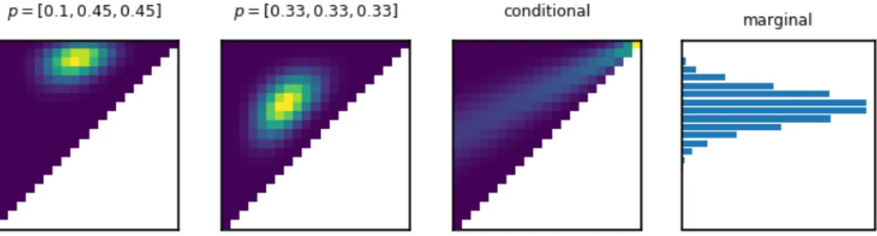
Figure 1.2:Multinomial distribution p(X,Y)withn=20and different categorical distribu-tions p, as well as the conditional distribution p(X|Y) and the marginal distribution p(X)

of the second multinomial distribution.

describes the probability of having k successes in nexperiments, where p is the Bernoulli distribution of success and non-success for a single experiment. This parametric repre-sentation of a distribution with n discrete values only has two parameters, i.e., p and n. Consequently, the range of distributions that can be represented is limited. Figure 1.1 shows the probability masses with n =20 for different values of p. The single degree of freedom in this representation with the parameterponly allows to shift the single mode of the distribution betweenk=0for p→0and k=nfor p→1. An example of a multivari-ate, parametric, discrete probability distribution is the multinomial distribution. Now, the underlying experiment has not a Bernoulli distribution with two possible outcomes (’suc-cess’ and ’no suc(’suc-cess’), but a categorical distribution (also multinoulli distribution) with K

possible outcomes. For an experiment with 3 possible outcomes x,y,z, the multinomial distribution has two random variablesX,Y which count the number of the respective out-comes x and y inntrials. Figure 1.2 depicts the multinomial distribution forn=20trials with two different categorical distributions, as well as the conditional distribution p(X|Y)

and the marginal distribution p(X)which are obtained by conditioning and marginalizing, respectively, the second multinomial distribution.

(21)

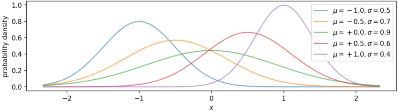
Figure 1.3:Probability density of a normal distribution for different values ofµandσ.

1.1.2 Continuous Probability Distributions

Continuous probability distributions are defined by cumulative distribution functions (cdf) which describe the probability that the random variableX is less than a given value x. The derivative of the cdf is the probability density function (pdf) which gives the probability mass for an infinitesimal value of the sample space Ω.

Continuous probability distributions usually do require parametric models as representa-tion. Besides the continuous uniform distribution, the most prominent example is probably the Gaussian distribution, also called the normal distribution, that is defined by the pdf

N(x;µ,σ) = p 1 2πσ2exp −(x−µ) 2 2σ2 . (1.3)

The parametersµandσallow to move the mode of the distribution and to scale the width, respectively. Figure 1.3 depicts normal distributions for different values ofµandσ.

Many other parametric continuous distributions exist, however, they usually share the common property that they have their probability mass distributed around a single mode. Exceptions are, for example, the bimodal beta and arcsine distributions which have two modes, one at each limit of the sample space. Most of these distributions have two or even only one parameter.

In the multivariate case with k random variables, the Gaussian distribution has the probability density function

N(x;µ,Σ) = _p 1 (2π)k_|Σ_|exp −1 2(x−µ) üΣ−1(_x₋µ) , (1.4)

where x andµarek-dimensional vectors andΣ_∈_Rk×k is the covariance matrix. If we par-tition the random variables into two subsetsX₁andX₂, we get the conditional distribution of X₁given X₂with pdf

p(X1=x1|X2=x2) =N(x1;µ1+Σ12Σ22−1(x2−µ2),Σ11−Σ12Σ−221Σ21). (1.5) 1.1 Probability Distributions and their Representations 5

(22)

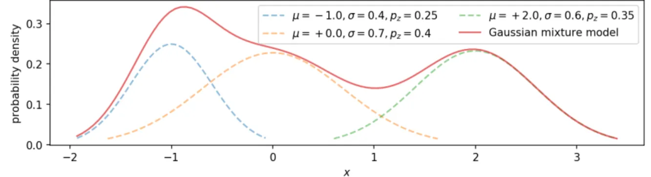
Figure 1.4:Gaussian mixture model with three components.

Here, Σ₁₁, Σ₂₂, and Σ₁₂ are the covariance matrices of the two subsets and the cross-covariance matrix, respectively. A marginal distribution of the subset can be obtained by dropping the remaining variables from mean and covariance, i.e., p(X₁ = x₁) =

N(x₁;µ₁,Σ11).

Mixture Models, Histograms and Kernel Density Estimation

Modeling distributions with more than one mode, i.e., bimodal or especially multi-modal distributions, requires more advanced, often hierarchical approaches such asmixture mod-els. A mixture model consists of multiple, but a fixed number of components. These components are usually continuous, parametric distributions, for example Gaussian distri-butions. Mixture models furthermore assume a latent variable zi that determines which

component is responsible for each sample x_i. A discrete distributionp(z_i)models the prior probability over the latent variables. By using normal distributions as components we obtain a Gaussian mixture model with pdf

p(x) =

N

X

i=1

N(x;µ_i,σ_i)p(z_i). (1.6)

Figure 1.4 shows a mixture model with three Gaussian components. Learning such mixture models from data is not trivial and requires techniques such as the iterative expectation-maximization algorithm to find locally optimal parameters. Another learning approach for mixture models is spectral learning. However, this approach assumes that the individual components are well separated [1].

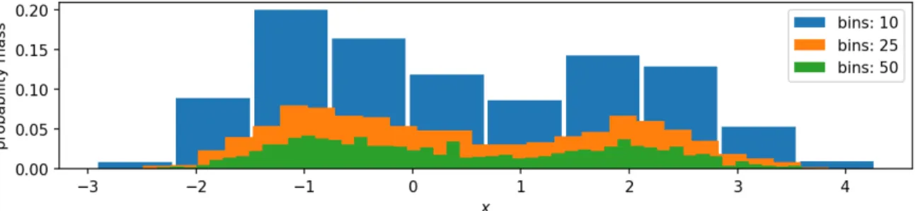
Alternatively,histogramsestimate probability distributions by discretization of the sam-ple space into equidistant bins and estimate the probability of each discrete state by count-ing the samples that fall into each of these bins. The most prevalent issue of histograms is however the exponential growth of the number of parameters with the dimensionality of the data. A trade-off between accuracy, i.e., small bins, and efficiency in the number of parameters and the number of samples that are required to get a good estimate of the dis-tribution, i.e., large bins, is necessary. Figure 1.6 shows a representation of the Gaussian mixture model using histograms with different bin sizes estimated from 1000 samples.

(23)

Figure 1.5: 1000 samples drawn from the Gaussian mixture model. For visualization the samples are randomly distributed between zero and the probability density value at their location.

Figure 1.6: Histograms generated from 1000 samples taken from the Gaussian mixture model (c.f. Figure 1.4) with different numbers of bins.

A non-parametric extension of histograms is kernel-density estimation. Here, the pdf is a linear combination of kernel functions k that are centered at the i.i.d. samples x_i from which we want to estimate the density, i.e.,

˜ p(x) = 1 n N X i k(x,xi). (1.7)

In this context, the term kernel function refers to a positive function that integrates to 1. Examples are the uniform kernel, the triangular kernel, or the Gaussian kernel. In the case of a Gaussian kernel, kernel density estimation is related to a Gaussian mixture-model with a mixture component centered at each sample point and a common variance which is also called bandwidth in the case of a kernel function. Since we assume the samples to be i.i.d., the discrete distribution over the mixture components is a uniform distribution

p(x_i) = 1_n. For mixture models the problem is to find an optimal number of components and a good initialization before optimizing the parameters of each component and of the prior distribution. In kernel density estimation, this problem is transferred to finding an optimal bandwidth of the kernel function.

The density of a joint probability distribution can be estimated by using a product kernel or a suitable kernel function for all variables, e.g., a multivariate Gaussian kernel. From 1.1 Probability Distributions and their Representations 7

(24)

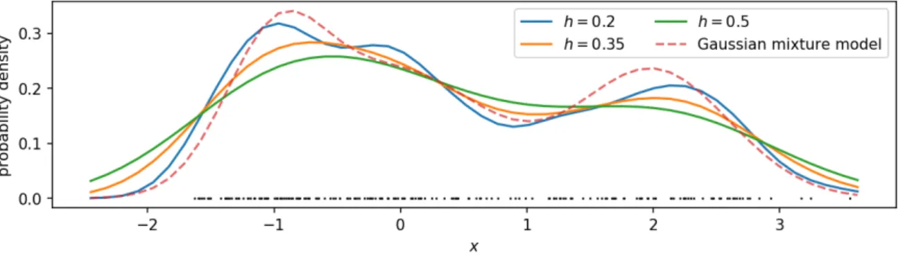
Figure 1.7: Kernel density estimation of the Gaussian mixture model using 200 samples (depicted as black dots) with a Gaussian kernel.

the joint kernel density estimate and a marginal density estimate, we can obtain the kernel density estimate of a conditional distribution by applying Equation 1.1 as

˜ p(x_|y) = ˜p(x,y) ˜ p(y) = PN i k(x,xi)g(y,yi) PN i g(y,yi) . (1.8)

Embedding Probability Distributions into Reproducing Kernel Hilbert Spaces

An alternative representation of probability distributions, which is related to the kernel density estimate, is the non-parametric embedding of a probability distribution into a re-producing kernel Hilbert space [100]. Note that the term kernel has in this case a more restricted meaning than in the case of kernel density estimation. In this case, a kernel, specifically a reproducing kernel, is a symmetric, positive definite function. The embed-dings of probability distributions into reproducing kernel Hilbert spaces and a framework for inference allow us to deduct conclusions using sample-based representations of arbi-trary distributions.

Intuitively, a Hilbert space is an extension of the well known two- or three-dimensional Euclidean space to high-dimensional or even infinite dimensional vector spaces. An ex-ample for such infinite dimensional Hilbert spaces is the space of functions, i.e., infinite dimensional vectors that contain for each element of the domain the corresponding func-tion value in the image. In addifunc-tion, a Hilbert space has an inner product that allows to measure distances and angles between its elements. For a reproducing kernel Hilbert space

H_k, this inner product〈·,·〉is implicitly defined by a reproducing kernel, withk:Ω×Ω→R

and k(x,y) =:〈ϕ(x),ϕ(y)_〉, whereϕ(x)is a feature mapping into a possibly infinite di-mensional space, intrinsic to the kernel function. An example for such a kernel function with intrinsic, infinite dimensional feature vectors is the Gaussian kernel. Due to the re-producing property of the kernel, all elements f of the RKHS can be reproduced by k in the sense that the outcome f(x) of the function for a specific value x can obtained by an evaluation of the kernel function [3], i.e., f(y) =_〈f,φ(y)_〉for any f _∈H_k. Based on the

(25)

representer theorem [87] and the reproducing property, the elements f of an RKHS H_k

can then be written as

f(·) = n X i=1 αik(xi,·) = n X i=1 αi〈ϕ(xi),ϕ(·)〉=αüΥ ü xϕ(·), (1.9)

with the weightsα_i∈Rand whereΥx = [ϕ(x1), . . . ,ϕ(xn)]denotes the feature matrix of

samples x_i.

The embedding of a marginal density p(X) into an RKHS is defined as the expected feature mapping

µX :=EX[ϕ(X)] =

Z ΩX

ϕ(X)p(X)dX, (1.10) also called the mean map[100]. Using a finite set of i.i.d. samples from p(X), the mean map can be estimated as

ˆ µX = 1 n n X i=1 ϕ(x_i) = 1 nΥ ü x1n, (1.11)

where Υ_x is the feature matrix of the samples from the distribution and 1_n ∈ Rn is an n

dimensional vector of ones. Because of the reproducing property of the kernel function, computing the expectation of a function which is an element of the same RKHS resolves to simple matrix operations. On the other hand, obtaining the probability of a single outcome or higher order statistics of the distributions is not straight forward. A joint distribution

p(X,Y)of the random variablesX andY can be embedded in a tensor product reproducing kernel Hilbert spaceH_k_×H_kas the expected tensor product of the feature mappings [100] as C_{X Y} :=EX Y [ϕ(X)⊗ϕ(Y)]−µX ⊗µY (1.12) = Z ΩX Z ΩY (ϕ(X)₋µ_X)_⊗(ϕ(Y)₋µ_Y)dXdY, (1.13)

where we use _⊗ to denote the tensor product (or outer product) of two vectors. This embedding is also called the centered covariance operator. The finite sample estimator is given by ˆ C_{X Y} = 1 m m X i=1 ϕ(x_i)_⊗ϕ(y_i)₋µˆX ⊗µˆY, (1.14)

assuming a set of m i.i.d. samples D = (x₁,y₁), . . . ,(x_n,y_n) from the joint distribu-tion p(X,Y). The embedding of a conditional distribution P(Y|X) is not like the mean map a single element of the RKHS, but rather a family of embeddings where there is one embedding for each realization of the conditioning variable X. To obtain the conditional distribution for a specific valueX =x_∗, Song et al. [104] define theconditional embedding 1.1 Probability Distributions and their Representations 9

(26)

operator C_Y_|_X which, if applied to the feature mapping of x_∗ returns the embedding of

P(Y|X =x_∗)

µY|x_∗ :=EY|x[φ(Y)] =CY|Xϕ(x∗). (1.15) Using a set of samples D = (x₁,y₁), . . . ,(x_n,y_n) , the conditional embedding operator can be derived from a least-squares objective [33] as

ˆ

C_Y_|_X =Φ(K_{x x} +λI_n)−1Υü

x, (1.16)

with the feature matrices Φ := [φ(y₁), . . . ,φ(y_n)] and Υ_x := [ϕ(x₁), . . . ,ϕ(x_n)], the Gram matrix K_{x x} =Υü

xΥx ∈R

n×n_{, the regularization parameter}_λ_{, and the identity matrix}

I_n∈Rn×n. With the feature mapping of the realization x∗ this results in µY|x_∗ =CˆY|Xϕ(x∗) =Φ(Kx x +λIn)− 1_Υ_ü xϕ(x∗) =Φ(Kx x +λIn)− 1_k x_∗, (1.17) where k_x

∗ is the kernel vector of the samples [x1, . . . ,xn] and the realization x∗. As the kernel matrices in the inverse and the kernel vector of the realization are finite, the embedding of the conditional distribution can be represented as a weighted sum of feature mappings µY|x_∗ =Φα= n X i=1 αiφ(yi), (1.18)

with the finite weight vectorα= (K_{x x} +λI_n)−1k_x ∗ ∈R

n_.

1.2 State Estimation with Models Learned from Data

The framework for nonparametric inference [103, 100, 20]—which is based on the em-beddings of distributions discussed above—allows to perform inference on arbitrary prob-ability distributions. High-dimensional embeddings in reproducing kernel Hilbert spaces (RKHS) are manipulated by kernelized inference rules. The conditional embedding oper-ator is used to derive the kernel sum rule, the kernel product rule, and the kernel Bayes’ rule (KBR). However, the computational demands of the conditional embedding operator and of the KBR do not scale well with the number of samples used in their estimators. In addition, the KBR often suffers from numerical instabilities.

In the first part of this thesis, I propose two additions to the framework for non-parametric inference to address these issues. First, I present a sparsification technique for the conditional embedding operator based on the least-squares objective. This spar-sification allows to learn a conditional embedding operator only on a subset of the data points while still leveraging from the full data set. I call this new approach the subspace conditional embedding operator. This work has been presented at the Large-Scale Kernel Learning Workshop at ICML 2015 [28]. Second, I present the kernel Kalman rule (KKR) as an alternative to the KBR. The derivation of the KKR follows from the clear objective of recursive least squares and is inspired by the well known Kalman filter. Based on the

(27)

KKR, I present the kernel Kalman filter (KKF) which uses RKHS embeddings to represent its belief state and learns the system and observation models as conditional embedding operators from data. I further derive the kernel forward backward smoother (KFBS) based on a forward and backward KKF and a smoothing update in Hilbert space. In addition, I derive the KKR, the KKF and the KFBS based on the subspace conditional embedding operator to leverage from the improved scalability with respect to the number of samples used for learning. I demonstrate on nonlinear state estimation tasks that my approaches provide a significantly improved estimation accuracy while the computational demands are considerably decreased. The work on the KKR, the KKF, and the KFBS is under review at the Machine Learning Journal [24] and has been presented at the AAAI Conference on Artificial Intelligence 2017 [29].

1.3 Swarm Representations for Learning Policies

In the second part of this thesis, I use the RKHS embeddings of probability distributions to represent the state of a robot swarm by its generative distribution. Swarm robotics investigates how a large population of robots with simple actuation and limited sensors can collectively solve complex tasks. One particular interesting application with robot swarms is autonomous object assembly. Such tasks have been solved successfully with robot swarms that are controlled by a human operator using a global control signal [85]. The application of such problem settings is mainly in the field of nano-robotics. Here, self-propelled, magnetotactic bacteria are used as agents [61] for the manipulation of nano-structures, for example drug containers. These bacteria have flagatella for propulsion and their orientation can be controlled by a magnetic field.

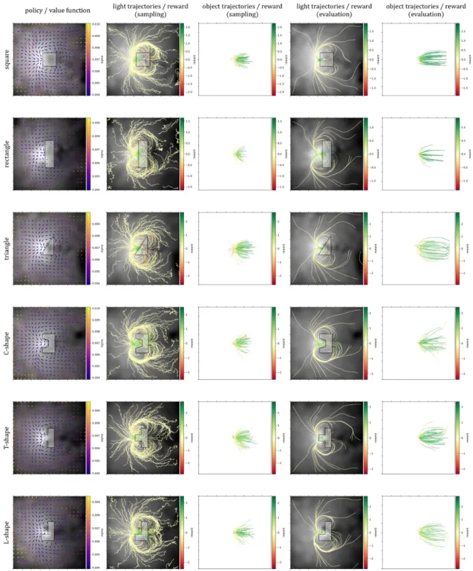
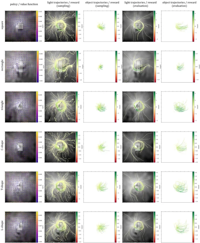
I propose a method to solve such assembly tasks autonomously based on policy search methods. Hereby, the assembly process is split into two subtasks: generating a high-level assembly plan and learning a low-level object movement policy. The high-level assembly policy plans the trajectories for each object and the low-level object movement policy controls the trajectory execution. Learning the object movement policy is challenging as it depends on the complex state of the swarm which consists of an individual state for each agent. To approach this problem, I introduce a representation of the swarm which is based on Hilbert space embeddings of distributions. The proposed representation is invariant to the number of agents in the swarm as well as to the allocation of an agent to its position in the swarm. These invariances make the learned policy robust to changes in the swarm and also reduce the search space for the policy search method significantly. I show that the resulting system is able to solve assembly tasks with varying object shapes in multiple simulation scenarios and evaluate the robustness of our representation to changes in the swarm size. Furthermore, I demonstrate that the policies learned in simulation are robust enough to be transferred to real robots. This work is under review at Advanced Robotics [22] and has been presented at the International Conference on Robotics and Automation (ICRA) 2018 [27]. It has been furthermore presented as extended abstract and as workshop contribution at the International Conference on Autonomous Agents and Multiagent Systems 2017 [26] and at the MALIC workshop at the Annual Conference on Neural Information Processing Systems 2016.

(28)

1.4 Learning Deep Representations for Sets of Homogeneous Inputs

Non-parametric, kernel-based methods for state estimation and prediction provide a versa-tile framework for inference on arbitrary shaped probability distributions. The problem of parameter learning is shifted to the problem of hyper-parameter learning with the promise of obtaining a more robust and better generalizing machine learning method. In fact, the ability of kernel methods to generalize well to unseen data trades off against the ability to model non-smooth functions.

In the recent years, neural networks have seen a revival due to the availability of mas-sive amounts of data and the computational resources to process this data in a reasonable amount of time. Besides the applications of neural networks in supervised learning for regression and classification problems, deep learning has also found its way into the field of reinforcement learning. Using the methods of deep reinforcement learning (DRL), ma-chines are able to learn complex control strategies directly from high dimensional obser-vations and in large state spaces [68, 95, 58].

In the third part of my thesis, I investigate how we can employ the idea of mean embed-dings in the realm of deep reinforcement learning. Specifically, I want to learn policies for object manipulation with a robot swarm. Neural networks usually have a predefined struc-ture which requires that the number of inputs and outputs is known in advance. In the case of swarms this is a severe limitation, as we might not always have the same number of agents in the swarm. However, also in other situations we might have to deal with vari-able numbers of homogeneous observations, as for example point clouds. Furthermore, such data has usually no ordering (i.e., if we exchange two swarm agents, we still have se-mantically the same state of the swarm, if we exchange two points in a point cloud, it still represents the same 3D structure) which cannot be exploited by standard neural network architectures. I present a structure, called the deep M-embeddings which are inspired by the kernel mean embeddings and allow for a compact representation of a variable set of homogeneous inputs as a feature vector of fixed size. In experimental evaluations, I show that this representation allows to learn complex policies in a multi-agent environment out-performing a standard multi-layer perceptron both in the achieved average episode return and in sample efficiency. This work has been submitted to Swarm Intelligence [23].

1.5 Challenges Addressed by the Contributions of this Thesis

In this thesis, I present novel approaches for state estimation and state representation using the concept of non-parametric mean embeddings. In this section, I want to discuss the challenges addressed in this thesis and refer to the chapters of this thesis in which I present the specific approaches.

A major challenge for state representation is imposed byhigh dimensionaldata. Yet, such data is often located on a much lower dimensional manifold of the high dimensional space. Identifying such manifolds and the corresponding projections that map the data to a lower dimensional space is a hard task. Kernel-based methods address this problem through identifying the manifold of the data by learning the representation and models directly from samples. However, to find good kernel machines requires proper settings of the hyper-parameters. In Chapter 2, I present additions to the framework for non-parametric

(29)

Challenge Addressed by Chapter

High dimensionality • Kernel Kalman Rule 2

• Deep M-Embeddings 4

Partial observability • Kernel Kalman Rule 2

• Swarm Kernel 3

Sample complexity • Subspace Conditional Embedding Operator 2

Permutation invariance • Swarm Kernel 3

Table 1.1:Challenges addressed in this thesis, proposed approaches and references.

inference [103] that address this problem. The presented kernel Kalman rule, alleviates the process of hyper-parameter identification by being more sample efficient and thus allowing for a faster optimization than existing techniques. The deep M-embeddings which I present in Chapter 4, address the issue of high dimensional state spaces by introducing a compact representation for sets of observations that allows to learn the parameters of neural network policies more sample efficient than with a standard multi-layer perceptron. A second challenge of state estimation is partial observability. Partial observability can arise from two reasons: occlusions in the sensory system or parts of the state are hard or impossible to measure. Both issues are addressed by the kernel Kalman filter presented in Chapter 2. First, the proposed kernel Kalman filter allows to learn observation models that deal with partial observations which are integrated into the belief state. Second, latent variables in the system are identified by learning a probabilistic, multi-modal dynamics model in the high-dimensional feature space of the kernel function. In Chapter 3, I present a kernel function for swarms which also addresses the problem of partial observability. By representing the swarm as a distribution, the kernel is inherently able to deal with incomplete observations where we do not observe all the agents of the swarm. In a similar fashion, the deep M-embeddings presented in Chapter 4 also allow for a variable number of inputs to a neural network and thus can be used to deal with incomplete observations.

When using kernel methods, a major downside is the poor scaling with the number of data points used for training. I propose two approaches in this thesis to address the problem ofsample complexity. In Chapter 2, I present the subspace conditional embedding operator This addition to the framework for non-parametric inference allows to represent belief states in a much smaller subset from the whole sample set while still learning the operators from the full sample set. Based on the subspace conditional embedding operator, I further re-derive the kernelized inference rules of the framework for non-parametric inference. A second approach is presented in Chapter 4, in which I present the deep M-embeddings. Based on the deep learning techniques, I propose a method that allows to learn a compact feature representation from data which provides an improved sample complexity compared to a standard multi-layer perceptron.

(30)

When using probabilistic representations as state estimators to abstract from complex states, we often want permutation invariance. Given a set of observations, the order of the observations in the set is of no importance and, thus, the representation should be invariant to changes in this order. The representation for swarms which I present in Chap-ter 3 addresses this challenge. By representing the swarm as a distribution embedded into an RKHS, the representation is invariant to permutations of the single agents in the swarm. The deep M-embeddings address the same issue by representing sets of obser-vations with variable size and without order as a feature vector of fixed size in a neural network structure. Table 1.1 gives an overview about the challenges addressed in this thesis, the proposed approaches and in which parts of my theses they can be found.

(31)

2 The Kernel Kalman Rule

In this chapter, I address the problem of state estimation in unstructured and unknown en-vironments. Traditional state estimation methods require known models and make strong assumptions about the dynamics. Novel, versatile techniques should be able to deal with high dimensional observations and non-linear, unknown system dynamics. The recent framework for nonparametric inference [103] allows to perform inference on arbitrary probability distributions. High-dimensional embeddings of distributions into reproducing kernel Hilbert spaces (RKHS) are manipulated by kernelized inference rules, most promi-nently the kernel Bayes’ rule (KBR). However, the computational demands of the KBR do not scale well with the number of samples.

In this chapter, I propose two techniques to increase the computational efficiency of non-parametric inference. First, I derive the kernel Kalman rule (KKR) from a recursive least squares objective and propose the KKR as an alternative to the KBR to perform Bayesian updates on mean embeddings of distributions. Based on the KKR, I present the kernel Kalman filter (KKF) that embeds the belief state into an RKHS and learns the system and observation models from data. I further derive the kernel forward backward smoother (KFBS) based on a forward and backward KKF and a smoothing update in Hilbert space. Second, I present the subspace conditional embedding operator as a sparsification tech-nique that still leverages from the full data set. I apply this sparsification to the KKR and derive the corresponding sparse KKF and KFBS algorithms. I show on nonlinear state es-timation tasks that my approaches provide a significantly improved eses-timation accuracy while the computational demands are considerably decreased.

2.1 Introduction

The ability to reason about past, current and future states in continuous, partially ob-servable stochastic processes is a fundamental stepstone towards fully autonomos and intelligent systems. Such models are required in many applications as for example state estimation in case of incomplete sensory data, smoothing noisy data from mediocre sen-sors, or predicting future states from past and current observations.

Traditional state estimation techniques usually require analytical models of the under-lying system, are often limited to a set of models with a special structure, and require knowledge about the moments of the stochstic processes. When assuming linear Gaussian models with known mean and covariance for instance, the Kalman filter [49] yields the optimal solution. However, the required linear Gaussian models with known statistics im-pose a strong limitation to the applicability of this method. For more complex processes, approximate solutions have to be used instead. Examples are the extended Kalman filter [66, 98] or the unscented Kalman filter [47, 113]. These solution inherit the Gaussian representation of the belief state to which they apply the non-linear system dynamics. However, the Gaussian distribution with its unimodal nature is a strong assumption about 15

(32)

the belief state which leads to poor results for systems that require a more complex dis-tribution over possible states. Moreover, both the Kalman filter but also it’s extensions to non-linear systems, require that the dynamics of the systems are given as analytical mod-els. Yet, these analytical models are often hard to obtain or make simplifying assumptions about the system.

The recently introduced framework for nonparametric inference [103, 20] alleviates the problems of traditional state estimation methods for nonlinear systems. The basic idea of these methods is to embed the probability distributions into reproducing kernel Hilbert spaces (RKHS). These embeddings allow the representation of arbitrary probability dis-tributions using empirical estimators. Inference on the embedded distribution can then be performed efficiently and entirely in the RKHS using the kernelized versions of the sum rule, the chain rule, and the Bayes’ rule. Additionally, Song, Fukumizu, and Gretton [103] use the kernel sum rule and the kernel Bayes’ rule to construct the kernel Bayes’ filter (KBF). The KBF learns the transition and observation models from observed samples and can be applied to nonlinear systems with high-dimensional observations. However, the computational complexity of the KBR update does not scale well with the number of samples such that hyper-parameter optimization becomes prohibitively expensive. More-over, the KBR requires mathematical tricks that may cause numerical instabilities and also render the objective that is optimized by the KBR unclear.

In this paper, we present two approaches to overcome the limitations named above. First, we introduce the subspace conditional embedding operator. In contrast to the condi-tional embedding operator [104], this operator allows to estimate its empirical estimator with a much larger data set while maintaining computational efficiency. We further apply the subspace conditional embedding operator to the kernel sum rule, kernel chain rule and kernel Bayes rule to derive their subspace versions. We have presented these results at the large-scale kernel learning workshop at ICML 2015 [28].

Furthermore, we present the kernel Kalman rule (KKR) as an approximate alternative to the kernel Bayes’ rule. Our derivations closely follow the derivations of the innovation update used in the Kalman filter and are based on a recursive least squares minimization objective in a reproducing kernel Hilbert space (RKHS). The KKR does not perform an exact Bayesian update as it uses a regularization term in the least squares objective and assumes constant noise on the conditioning variable. While the update equations are for-mulated in a potentially infinite dimensional RKHS, we derive through application of the kernel trick and by virtue of the representer theorem an algorithm that uses only opera-tions of finite kernel matrices and vectors. We employ the kernel Kalman rule together with the kernel sum rule for filtering, which results in the kernel Kalman filter (KKF). In contrast to filtering techniques that rely on the KBR, the KKF allows to precompute ex-pensive matrix inversions which significantly reduces the computational complexity and which also allows us to apply hyper-parameter optimization for the KKF. This work has been presented at AAAI 2017 [29].

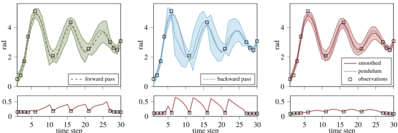
In addition to the KKF, we introduce thekernel forward backward smoother(KFBS) which computes the embedding of the belief state given all available observations from the past and the future. The kernel forward backward smoother combines the belief state embed-dings of a forward pass and a backward pass into smoothed embedembed-dings using Hilbert space operations. Both, the forward and the backward pass are realized by a KKF, where

(33)

the backward KKF operates backwards in time starting at the last observation. To scale gracefully with larger data sets, we rederive the KKR, the KKF and the KFBS with the subspace conditional operator [28].

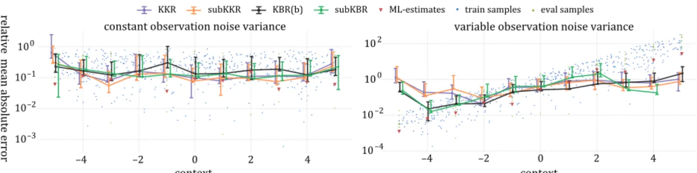
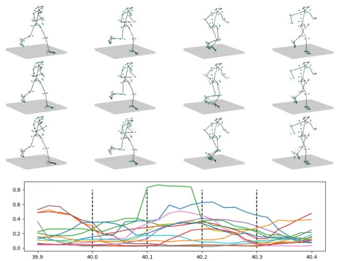
We compare our approach to different versions of the KBR and demonstrate its improved estimation accuracy and computational efficiency. Furthermore, we evaluate the KKR on a simulated 4-link pendulum task, on a human motion capture data set [117] and on data from a table-tennis setup [30].

2.1.1 Related Work

To the best of our knowledge the kernel Bayes’ rule exists in three different versions. It was first introduced in its original version by Fukumizu, Song, and Gretton [20]. Here, the KBR is derived, similar to the conditional operator, using prior modified covariance operators. These prior-modified covariance operators are approximated by weighting the feature mappings with the weights of the embedding of the prior distribution. Since these weights are potentially negative, the covariance operator might become indefinite, and thus, rendering its inversion impossible. To overcome this drawback, the authors have to apply a form of the Tikhonov regularization that decreases accuracy and increases the computational costs. A second version of the KBR was introduced by Song, Fukumizu, and Gretton [103] in which they use a different approach to approximate the prior-modified covariance operator. In the experiments conducted for this paper, this second version often leads to more stable algorithms than the first version. Boots, Gretton, and Gordon [8] in-troduced a third version of the KBR where they apply only the simple form of the Tikhonov regularization. However, this rule requires the inversion of a matrix that is often indefi-nite, and therefore, high regularization constants are required, which again degrades the performance. In our experiments, we refer to these different versions with KBR(b) for the first, KBR(a) for the second (order adapted from the literature), and KBR(c) for the third version. [103] propose in their framework for nonparametric inference to combine the KBR with the kernel sum rule to obtain the kernel Bayes filter (KBF). The kernel Kalman filter presented in this work is closely related to this, as we simply replace the KBR with the KKR. We compare to the KBF in our experiments. [70] recently proposed the nonpara-metric kernel Bayes smoother. This approach builds on top of the kernel Bayes filter, which is used to compute the estimates of a normal forward pass. The smoothing update is then obtained by propagating the embeddings backwards in time without performing a second filtering pass.

For filtering tasks with known linear system equations and Gaussian noise, the Kalman filter (KF) yields the solution that minimizes the squared error of the estimate to the true state. Two widely known and applied approaches to extend the Kalman filter to non-linear systems are the extended Kalman filter (EKF) [66, 98] and the unscented Kalman filter (UKF) [113, 47]. Both, the EKF and the UKF, assume that the non-linear system dynamics are known and use them to update the prediction mean. Yet, updating the prediction covariance is not straightforward. In the EKF the system dynamics are linearized at the current estimate of the state, and in the UKF the covariance is updated by applying the system dynamics to a set of sample-points (sigma points). While these approximations