Adaptive Pointwise Estimation in Time-Inhomogeneous Time-Series Models

No. 2007–35

ADAPTIVE POINTWISE ESTIMATION IN

TIME-INHOMOGENEOUS TIME- SERIES MODELS

By P.

Č

ížek, W. Härdle, V. Spokoiny

May 2007

time-inhomogeneous time-series models

P. ˇ

C´ıˇzek,

W. H¨ardle,

and V. Spokoiny

Abstract

This paper offers a new method for estimation and forecasting of the linear and nonlinear time series when the stationarity as-sumption is violated. Our general local parametric approach par-ticularly applies to general varying-coefficient parametric models, such as AR or GARCH, whose coefficients may arbitrarily vary with time. Global parametric, smooth transition, and change-point models are special cases. The method is based on an adap-tive pointwise selection of the largest interval of homogeneity with a given right-end point by a local change-point analysis. We con-struct locally adaptive estimates that can perform this task and investigate them both from the theoretical point of view and by Monte Carlo simulations. In the particular case of GARCH esti-mation, the proposed method is applied to stock-index series and is shown to outperform the standard parametric GARCH model.

JEL codes: C13, C14, C22

Keywords: adaptive pointwise estimation, autoregressive models, conditional het-eroscedasticity models, local time-homogeneity

∗_{Dept. of Econometrics & OR, Tilburg University, P.O.Box 90153, 5000LE Tilburg, The}

Netherlands.

†_{Humboldt-Universit¨at zu Berlin, Spandauerstrasse 1, 10178 Berlin, Germany.} ‡_{Weierstrass-Institute, Mohrenstr. 39, 10117 Berlin, Germany.}

1

Introduction

A growing amount of econometrical research is devoted to modeling macroeco-nomic and financial time series and their volatility, which measures dispersion at a point in time (e.g., conditional variance). Although many economies and fi-nancial markets have been recently experiencing many shorter and longer periods of instability or uncertainity such as Asian crisis (1997), Russian crisis (1998), start of the European currency (1999), the “dot-Com” technology-bubble crash (2000–2002), or the terrorist attacks (September, 2001) and the war in Iraq (2003), mostly used econometric models are based on the assumption of time homogene-ity. This includes linear and nonlinear autoregressive and moving-average models (ARMA) and conditional heteroscedasticity models such as ARCH (Engel, 1982) and GARCH (Bollerslev, 1986), stochastic volatility models (Taylor, 1986), as well as their combinations such as AR-GARCH or ARCH-in-mean (Engle et al., 1987). On the other hand, the market and institutional changes have long been as-sumed to cause structural breaks in macroeconomics and financial time series, which was confirmed, for example, in data on GDP (McConnell and Perez-Quiros, 2000), money demand (Wolters et al., 1990), stock prices (Andreou and Ghysels, 2002; Beltratti and Morana, 2004), and exchange rates (Herwatz and Reimers, 2001). There even seems to be causal relationship between shocks and structural changes in macroeconomic and financial indicators (Beltratti and Morana, 2006). Moreover, ignoring these breaks can adversely affect the modeling, estimation, and forecasting as suggested by Diebold and Inoue (2001), Mikosch and Starica (2004), Pesaran and Timmermann (2004), and Hillebrand (2005), for instance. Such findings led to the development of the change-point analysis in the context of linear time-series and conditional-heteroscedasticity models; see for example, Chen and Gupta (1997), Bai and Perron (1998), Kokoszka and Leipus (2000), Andrews (2003), Perron and Zhu (2005), and Andreou and Ghysels (2006).

An alternative approach lies in relaxing the assumption of time homogeneity and allowing some or all model parameters to vary over time (Fan and Zhang, 1999; Cai et al., 2000; Fan et al., 2003). Without structural assumptions about

the transition of model parameters over time, time-varying coefficient models have to be estimated nonparametrically, for example, under the identification condition that their parameters are smooth functions of time (e.g., Orbe et al., 2005). In this paper, we follow a more general strategy based on the assumption that a time series can be locally, that is over short periods of time, approximated by a parametric model. As suggested by Spokoiny (1998), such a local approximation can form a starting point in the search for the longest period of stability (homogeneity), that is, for the longest time interval in which the series is described well by a given parametric model. In the context of the local constant approximation, this strategy was employed for volatility modeling by H¨ardle et al. (2003) and Mercurio and Spokoiny (2004). Our aim is to generalize this approach so that it can identify intervals of homogeneity for any parametric model irrespective of its complexity.

In contrast to the local constant approximation of the volatility of a process (Mercurio and Spokoiny, 2004), the main benefit of the proposed generalization consists in the possibility to apply the methodology to a much wider class of models and to forecast over a longer time horizon. The reason is that approximating the mean or volatility process is in many cases too restrictive or even inappropriate and it is fulfilled only for short time intervals, which precludes its use for longer-term forecasting. On the contrary, parametric models like ARMA and GARCH mimic the majority of stylized facts about macroeconomic and financial time series and can reasonably fit the data over rather long periods of time in many practical situations. Allowing for time dependence of model parameters offers then much more flexibility in modeling real-life time series, which can be both with or without structural breaks since global parametric models are included as a special case.

Moreover, the proposed adaptive local parametric modeling unifies the change-point and varying-coefficient models. First, since finding the longest time-homogen-eous interval for a parametric model at any point in time corresponds to detecting the most recent point in a time series, this approach resembles the change-point modeling as in Bai and Perron (1998) or Mikosch and Starica (1999, 2004), for instance, but it does not require prior information such as the number of

changes. Additionally, both the traditional structural-change tests (e.g., Bai and Perron, 1998) and the end-of-sample stability tests (e.g., Chu et al., 1996; An-drews, 2003) require that the number of observations before each break point is large (and can grow to infinity) as these tests rely on asymptotic results. This is not very realistic especially in macroeconomic time series (e.g., for yearly data). On the contrary, the proposed pointwise adaptive estimation does not rely on asymptotic results and does not thus place any requirements on the number of ob-servations before, between, or after any break point. Second, since the adaptively selected time-homogeneous interval used for estimation necessarily differs at each time point, the model coefficients can arbitrarily vary over time. In comparison to varying-coefficient models assuming smooth development of parameters over time (Cai et al., 2000), our approach however allows for structural breaks in the form of sudden jumps in parameter values.

Although seemingly straightforward, extending Mercurio and Spokoiny (2004)’s procedure to the local parametric modeling is a nontrivial problem, which requires new tools and techniques. This is especially true for nonlinear and data-demanding models such as GARCH. The reason is that, at each time point, the procedure starts from a small interval, where local parametric approximation holds, and then iteratively extends this interval and tests it for time-homogeneity until a structural break is found or data exhausted. Hence, a model has to be initially estimated on very short time intervals (e.g., 5 or 10 observations). Using standard testing methods, such a procedure might be feasible for simple parametric models, such as the local constant approximation used by Mercurio and Spokoiny (2004), but it is hardly possible for more complex parametric models such as GARCH that gen-erally require rather large samples for reasonably good estimates. Therefore, we use an alternative and more robust approach to local change-point analysis based on Spokoiny and Chen (2007), which relies on a finite-sample theory of testing a growing sequence of historical time intervals on homogeneity against a change-point alternative. We generalize their results to general time-series models, includ-ing autoregressive and conditional-heteroscedasticity models, and demonstrate the

feasibility and stability of the proposed method.

The rest of the paper is organized as follows. In Section 2, we discuss the two main ingredients of the method: parametric estimation of autoregressive conditional-heteroscedasticity models and the test of homogeneity for these mod-els. Section 3 introduces the adaptive estimation procedure and discusses the choice of its parameters. Theoretical properties of the method are discussed in Section 4. In the specific case of the GARCH(1,1) model, a simulation study il-lustrates the performance of the new methodology with respect to the standard parametric and change-point models in Section 5. Applications to real stock-index series data are presented in Section 6. The proofs are provided in the Appendix.

2

Parametric time-series models

Consider a time series Yt in discrete time, t∈N. A standard way to model such

processes is based on one or another parametric specification. One frequently employed example is given by the autoregressive (AR) model:

Yt=γ0+

pm

X

i=1

γiYt−i+ηt, (2.1)

where {ηt}t∈N is a white noise process and θ = (γ0, . . . , γpm)

⊤ _{is a parameter}

vector. (The AR model can also be nonlinear.)

In financial applications, one often applies similar equations for the volatil-ity process which includes a large class of parametric models around the ARCH (Engle, 1982) and GARCH (Bollerslev, 1986) specifications:

Yt=σtεt, σ2t =ω+ pv X i=1 αiYt2−i+ qv X j=1 βjσt2−j, (2.2)

where {εt}t∈N is again a white noise process. A number of GARCH extensions

were proposed to make the model even more flexible; for example, EGARCH (Nel-son, 1991), QGARCH (Sentana, 1995), and TGARCH (Glosten et al., 1993) that account for asymmetries in a volatility process. All such

conditional-heteroscedast-icity models can be put into a common class of generalized linear volatility models: σt=g(Xt), Xt=ω+ pv X i=1 αih(Yt−i) + qv X j=1 βjXt−j, (2.3)

where g and h are known functions, Xt is a (partially) unobserved process

(structural variable) that models volatility coefficient σ2

t via transformation g,

and θ _{= (ω, α1, . . . , αpv, β1, . . . , βqv)}⊤ _{is a parameter vector. For example, the}

GARCH model (2.2) is described by g(u) =u and h(r) =r2_.

One can also combine the AR-type modeling (2.1) for the observables Yt and

the GARCH-type modeling (2.3) for the noise: with Zt=h(Yt) , the model reads

Yt = γ0+ pm X i=1 γtYt−i+ηt ηt = σtεt=g(Xt)εt, (2.4) Xt = ω+ pv X i=1 αiZt−i+ qv X j=1 βjXt−j.

This model class does not include ARMA and stochastic volatility models, or more generally, the Hidden Markov Chain models. An extension of our approach to such models is possible but involves a number of serious technical problems. However, the class (2.4) is sufficiently large to cover many applications.

We consider a general parametric set-up covering models (2.1)–(2.4), which can

be described as follows. Let the observed process Yt be progressively measurable

w.r.t. a filtration F = (Ft) and let Xt be a non-observed or partially observed

explanatory process which is predictable w.r.t. F, that is, Xt∼ Ft−1. In general,

both Yt and Xt can be multivariate. Our basic assumption is that the conditional

distribution of Yt given the “past” Ft−1 belongs to some given parametric family

P = (Pυ) , but the corresponding parameter υ depends on the explanatory vector

Xt and some parameter θ. We write this relation in the form

L Yt|Ft−1

= Pg(Xt) ∈ P, (2.5)

Xt = fθ(Yt−1, Xt−1), (2.6)

where Yt−1 _{means the past Y}

t−1, Yt−2, . . . of the process Yt, Xt−1 is defined

to note that, given the parameter θ_{, the observations Y1, . . . , Yt, and the}

pre-history X0_{, Y}0_{, one can uniquely reconstruct the process X}

t=Xt(θ) for t ≥1

by recurrently applying the relation (2.6) for Xt. Under ergodicity conditions,

the impact of the pre-history X0_{, Y}0 _{is not significant and we just fix it arbitrary.}

In the case of volatility modeling, Yt means the squared return at time t and

Pυ ∈ P is the distribution of a squared normal random variable with zero mean

and variance υ. The parametric assumption (2.6) means that the time-varying

volatility σ2

t =g(Xt) is a parametric function of the process Xt.

Model (2.5)-(2.6) is time homogeneous in the sense that the process Yt follows

the same structural equation at each time point. In other words, parameter θ _and

hence the structural dependence in Yt is constant over time. Even though

mod-els like (2.4) can often fit data well over a longer period of time, the assumption of homogeneity is too restrictive in practical applications: to guarantee sufficient amount of data for sufficiently precise estimation, these models are often applied for time spans of many years both in the case of macroeconomic data (e.g., due to low sampling frequency) and financial data (e.g., due to high data demands of GARCH models). On the contrary, the strategy pursued in this paper requires

only local time homogeneity, which means that at each time point t there is a

(possibly rather short) interval [t−m, t] , where the process Yt is well described

by model (2.5)-(2.6). This strategy aims then both at finding an interval of homo-geneity (preferably as long as possible) and at the estimation of the corresponding

parameter values, which then enable predicting Yt and Xt.

Now, Section 2.1 describes in details the method of parameter estimation in the model (2.5)-(2.6). Its accuracy in finite samples is discussed in Section 2.2.

2.1

Parameter estimation

This section discusses the parameter estimation for model (2.5)-(2.6) using

obser-vations Yt from some time interval I = [t0, t1] . To give a specific example, we

can focus on the problem of volatility modeling with Pυ being the distribution of

υε2_{, where ε is standard normal. The process Y}

for volatility σ2

t = g(Xt) are described by equations (2.5)-(2.6). We write these

processes in the form Yt =Yt(θ) and Xt =Xt(θ) for t ∈ I. In the parametric

case, θ∗ _{denotes the underlying value of} θ_.

For estimating θ∗_{, we apply the quasi maximum likelihood (quasi-MLE)}

ap-proach under the assumption of Gaussian errors εt, which guarantees efficiency

under the normality of innovations and consistency under rather general moment conditions (Hansen, 1982; Hansen and Lee, 1994). The quasi log-likelihood for the

model (2.5)-(2.6) on an interval I can be represented in the form

LI(θ) =

X

t∈I

ℓ{Yt(θ), g(Xt(θ))}

with ℓ(y, x) = −0.5{log(x) +y2_{/x}. We define the quasi-MLE estimate eθ}

I of

the parameter θ _{by maximizing the log-likelihood LI(}θ_{) ,}

e θ_{I = argmax} θ_∈Θ LI(θ) = argmax θ_∈Θ X t∈I ℓ{Yt(θ), g(Xt(θ))}, (2.7)

and denote by LI(θeI) the corresponding maximum. Symbol Θ denotes the

para-metric space containing only parameter values ensuring ergodicity of process Yt.

2.2

Accuracy of parametric situation

This section discusses some specific properties of the proposed (quasi-)MLE

esti-mate eθ _{that apply for an arbitrarily long interval I (i.e., for an arbitrarily small}

or large sample size). This feature is very important for the proposed adaptive procedure because it starts the search for a structural break in parameter values

at very small intervals. For a given interval I, we now discuss the accuracy of

estimation by eθ_{I in the time-homogeneous situation when the process Yt follows}

a parametric model with the parameter vector θ∗ _{for all t ∈I.}

The main result concerning the quality of estimation of θ _{concerns the value}

of maximum LI(eθI) = maxθ_∈ΘL(θ) rather than the point of maximum θe. More

precisely, we consider difference LI(eθI,θ∗) =LI(eθI)−LI(θ∗) . By definition, this

value is non-negative and represents the deviation of the maximum of the

how the accuracy of estimation of the parameter θ∗ _by eθ_{I relates to the value}

LI(eθI,θ∗) . We will also see that the bound for LI(θeI,θ∗) yields the confidence

set for the parameter θ∗_{, which is then used for the employed change-point test.}

Theorem 2.1 (Spokoiny, 2007). Assume that the process Yt follows the model

(2.5)–(2.6) with the parameter θ∗ _{∈Θ. Let the parameter set Θ be compact and} the function fθ(x) be continuously differentiable w.r.t. θ. Let the process X_t(θ)

belong to a compact set X for all t ∈ N and θ _{∈ Θ and g(x) is smooth and} separated away from zero on X . Then there are some λ >0 and values e(λ,θ∗₎ and e(λ) depending on only fθ, g, and X such that

logEθ∗exp

λLI(eθI,θ∗) ≤e(λ,θ∗)≤e(λ).

Moreover, for any z>0, it holds that

Pθ∗ L_I(eθ_I,θ∗)>z≤expe(λ)−λz , (2.8)

and for any r > 0 and every θ∗ _{∈ Θ, there is a constant Rr(}θ∗_{) depending on} X and r only such that

Eθ∗ LI(eθI,θ∗) r ≤Rr(θ∗)≤Rr.

Remark 2.1. The condition that Xt(θ) is bounded can be easily relaxed to the

condition that Xt(θ) is ergodic and thus belongs to a bounded set with a high

probability but the corresponding formulation is more involved. A special case of this result can be found in Spokoiny and Chen (2007).

One very attractive feature of Theorem 2.1, formulated in the following corol-lary, is that it enables constructing the exact non-asymptotic confidence sets and

testing the parametric hypothesis on the base of the fitted log-likelihood LI(eθI,θ) .

This feature is especially important for our procedure presented in Section 3.

Corollary 2.1. Under the assumptions of Theorem 2.1, let the value zα

ful-fill e(λ,θ∗_{) −λzα < logα for some α < 1. Then the random set EI(zα) =} {θ _{: LI(}eθ_I,θ_{) ≤ zα} is an α-confidence set for} θ∗ _{in the sense that} Pθ∗ θ∗ 6∈

EI(zα)

≤α.

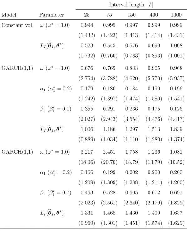
Table 1: Simulated mean values and standard deviations (in brackets, multiplied

by factor|I|1/2) of parameter estimates and likelihood differences LI(eθI,θ∗). The

parameters of a constant volatility model and two GARCH(1,1) models with

nor-mally distributed error terms are estimated for intervals I with 25 to 1000

obser-vations using 10000 simulated samples.

Interval length |I| Model Parameter 25 75 150 400 1000 Constant vol. ω (ω∗ _{= 1.0) 0.994 0.995 0.997 0.999 0.999} (1.432) (1.423) (1.413) (1.414) (1.431) LI(eθI,θ∗) 0.523 0.545 0.576 0.690 1.008 (0.732) (0.760) (0.783) (0.893) (1.001) GARCH(1,1) ω (ω∗ _{= 1.0) 0.676 0.765 0.833 0.905 0.968} (2.754) (3.788) (4.620) (5.770) (5.957) α1 (α∗1 = 0.2) 0.179 0.180 0.184 0.190 0.196 (1.242) (1.397) (1.474) (1.580) (1.541) β1 (β1∗ = 0.1) 0.355 0.291 0.236 0.175 0.126 (2.027) (2.943) (3.554) (4.476) (4.417) LI(eθI,θ∗) 1.006 1.186 1.297 1.513 1.839 (0.889) (1.034) (1.110) (1.280) (1.374) GARCH(1,1) ω (ω∗ _{= 1.0) 3.217 2.451 1.758 1.236 1.081} (18.06) (20.70) (18.79) (13.79) (10.52) α1 (α∗1 = 0.2) 0.166 0.199 0.202 0.200 0.200 (1.209) (1.309) (1.288) (1.211) (1.200) β1 (β1∗ = 0.7) 0.463 0.528 0.605 0.672 0.691 (2.023) (2.561) (2.640) (2.179) (1.829) LI(eθI,θ∗) 1.331 1.468 1.430 1.499 1.637 (0.969) (1.301) (1.451) (1.574) (1.629)

The benefits of considering the distance LI(eθI,θ∗) and the result of

Theo-rem 2.1 can be illustrated by a small simulation study. Consider the constant volatility and GARCH(1,1) models with two different sets of parameters. In Ta-ble 1, estimation results are presented in terms of the mean and the normalized

standard deviation |I|1/2 _θe

I −θ∗

of the estimate θe_{I and in terms of the}

fit-ted log-likelihood LI(eθI,θ∗) . We see that for the constant volatility model, the

results are nicely in agreement with the root-n consistency of the estimate θe_I,

whereas for the GARCH(1,1) models, the results for small sample sizes are awful in the sense that the standard deviation of estimates is of order of the range of the parameter set. At the same time, the fitted log-likelihood demonstrates a very stable behaviour for all models and sample sizes.

As already mentioned, Theorem 2.1 gives a non-asymptotic and fixed upper

bound for the risk of estimation which applies to an arbitrary sample size |I|.

To understand the relation of this result to the classical rate result, we apply the standard arguments based on the quadratic expansion of the log-likelihood

L(eθ_,θ_{) . Let ∇}2_L(θ_{) denote the Hessian matrix of the second derivatives of}

L(θ_{) with respect to the parameter} θ_{. Then}

LI(eθI,θ∗) = 0.5 θeI−θ∗ ⊤ ∇2L(θ′ I) eθI−θ∗ , (2.9) where θ′

I is some point on the line connecting θ∗ and eθI. Under the usual

ergod-icity assumptions and for sufficiently large |I|, the normalized matrix |I|−1_∇2_L(θ)

is close to some matrix V2_{(θ) , which depends only on the stationary distribution}

of Xt(θ) and is continuous in θ. Then the result of the theorem approximately

means that kV(θ∗₎ eθ_I−θ∗_k2 _{≤z/|I| for some fixed constant z. In other words,}

the large deviation result of Theorem 2.1 yields the root-|I| consistency of the

MLE estimate eθ_I.

3

Adaptive nonparametric estimation

An obvious feature of the model (2.5)-(2.6) is that the parametric structure of the process is assumed constant over the whole sample and cannot thus incorporate

changes and structural breaks at unknown times in the model. A natural general-ization leads to models whose coefficients may vary with time. For example, Cai et al. (2000) considered the following varying-coefficient model

Yt=γ0(t) + p

X

i=1

γi(t)Yt−i+εt, (3.1)

where γ0(t), . . . , γp(t) are functions of time and have to be estimated from the

observations Yt. In general, one can assume that the structural process Xt

sat-isfies the relation (2.6) but the vector of coefficients θ _{may vary with the time t,}

θ ₌θ_{(t) . The estimation of the coefficients as functions of time is a hard}

prob-lem and it is possible only under some additional assumptions on these functions. Typical examples are given by (i) varying coefficients are smooth functions of time (Cai et al., 2000) and (ii) varying coefficients are piecewise constant functions (Bai and Perron, 1998; Mikosch and Starica, 1999, 2004).

Our local parametric approach differs from the commonly used identification

assumptions (i) and (ii). We assume that the observed data Yt are described

by a (partially) unobserved process Xt due to L Yt|Ft−1

∼ Pg(Xt), see (2.5),

and at each point T , there exists a historical interval I(T) = [t, T] in which

the process Xt “nearly” follows the parametric specification (2.6) (see Section 4

for details on what “nearly” means). This local structural assumption enables

us to apply well developed parametric estimation for data {Yt}t∈I(T) to estimate

the parameter θ ₌ θ_{(T) . The estimate} bθ ₌ bθ_{(T) leads to the value X}b_{T =}

fbθ(Y

T−1_{, X}T−1_{) of the process X}

t at T and can be used for further modeling,

for example, for forecasting the next value YT+1. Moreover, this assumption

includes the above mentioned “smooth transition” and “switching regime” models

as special cases: parametersbθ_{(T) vary over time asI(T) changes, and at the same}

time, discontinuities and jumps in bθ_{(T) as a function of time are possible.}

The idea of choosing the historical interval of homogeneity I(T) is to find

the longest interval I with the right-end point T , where data do not contradict

the hypothesis of model homogeneity. Starting at each time T with a very short

interval I = [t, T] , the search is done by successive extending and testing of

of homogeneity is not rejected for a given I, a larger interval is taken and tested again. This method strongly differs from that of Bai and Perron (1998) and Mikosch and Starica (1999) who try to detect all change points in a given time series. Our approach is local in the sense that it focuses on the local change-point analysis near the point of estimation or forecasting and tries to find only one change closest to the reference point.

In the rest of this section, we first rigorously describe the adaptive pointwise estimation procedure (Section 3.1), which relies on the test of time-homogeneity against a change-point alternative discussed in Section 3.2. Next, the choice of pa-rameters and implementation of the adaptive procedure is described in Section 3.3. Theoretical properties of the method are studied in Section 4.

3.1

Adaptive choice of the interval of homogeneity

This section proposes an adaptive method for the pointwise selection of the longest historical interval of homogeneity for the parametric model (2.6). For a given point

T , we aim to estimate the unknown parameter θ₌θ_{(T) from historical data Yt,}

t≤T . This procedure repeats for every current time point T as new data arrives.

The choice of the longest homogeneous interval at a given point T is done

by the multiscalelocal change point (LCP) detection procedure. The procedure is

based on a family of nested interval-candidates I0 ⊂I1 ⊂I2 ⊂. . .⊂IK =IK+1 of

the form Ik = [T −mk, T] , where T is the right-end point and mk is the interval

length growing with k. Every interval leads to the estimate eθ_{k =} θe_{Ik of the}

parameter θ _{from the interval Ik. The adaptive procedure selects one interval I}b

out of the given family and thus the corresponding estimate bθ ₌θe_b

I.

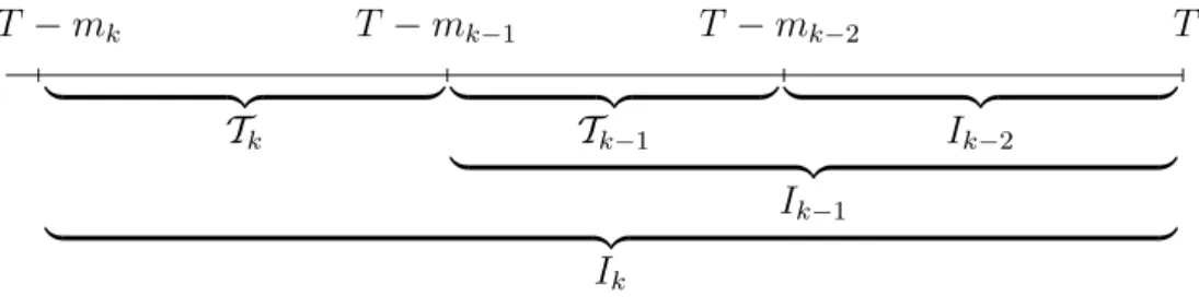
The idea of the proposed method is to sequentially screen each interval Tk =

Ik \ Ik−1 = [T − mk, T − mk−1[, k = 1, . . . , K, and check each point τ ∈ Tk

for a possible change-point location (see Section 3.2 for details of the test). The

interval Ik is accepted if no change point is detected within T1, . . . ,Tk (interval

I0 has to be so short that homogeneity can always be assumed). If the hypothesis

T −mk T −mk−1 T −mk−2 T | {z } Tk | {z } Tk−1 | {z } Ik−2 | {z } Ik−1 | {z } Ik

Figure 1: Choice of the intervalsIk and Tk

selects the latest accepted interval. The formal description reads as follows.

Start the procedure with k = 1 . Then (see Figure 1 for illustration)

1. test the hypothesis H0,k of no structural change within Tk using data from

testing interval Ik+1;

2. if no change points were found in Tk, interval Ik is accepted. Take the next

interval Tk+1 and repeat the previous step withk :=k+1 until homogeneity

is rejected or the largest possible interval IK = [T −mK, T] is accepted;

3. if H0,k is rejected for Tk, the estimated interval of homogeneity is the last

accepted interval Ib=Ik−1;

4. if the largest possible interval IK is accepted, we take Ib=IK.

In the description of the adaptive procedure above, Ibk = Ik is the latest

accepted interval after the first k steps of the procedure, provided that the

pro-cedure has not stop yet. The corresponding quasi-MLE estimate on Ik is then

b

θ_k=eθ_{Ik. The final adaptively selected interval I}b_{(T) at T is the latest accepted}

interval from the whole procedure, that is, Ib(T) =Ib. The corresponding adaptive

pointwise estimate bθ_{(T) is then defined as} θb_{(T) =}eθ_b

I(T).

3.2

Test of homogeneity against a change-point alternative

The main ingredient of the adaptive estimation procedure is the test of local

Let T be a tested historical interval. This means that we want to check every point of this interval for a possible change in the dependency structure.

The test statistic is based on the observations Yt from a larger testing interval

I of the form I = [T −m, T] . We consider the supremum likelihood ratio (LR)

test introduced by Andrews (1993). The null hypothesis for I means that the

observations {Yt}t∈I follow the parametric model (2.6) with a parameter θ =θ∗,

which yields the parametric estimate eθ_{I due to (2.7) and the corresponding fitted}

log-likelihood LI(eθI) . The change-point alternative given by the tested set T

can be described as follows. Every point τ ∈ T ⊂ I splits the interval I in two

subintervals J = [τ+1, T] and Jc _{=I\J = [T−m, τ] . A change-point alternative}

with a location at τ ∈ T(I) means that Yt follows the parametric model with

parameter θ_{J for t ∈ J and} θ_Jc for t ∈ Jc with θ_J 6= θ_Jc. Under such an

alternative, data {Yt}t∈I are associated with the log-likelihood LJ(θeJ)+LJc(eθ

Jc) .

To test against a single change-point alternative with a known fixed τ ∈ T ,

the LR test statistic can be used:

TI,τ = max θJ,θJ c∈Θ {LJ(θJ) +LJc(θ J)} −max θ_∈Θ LI( θ_{) =LJ(}θe_{J) +LJ}c(θe Jc)−L I(θeI).

Considering an unknown change point τ ∈ T , the test of homogeneity for intervals

I can be defined as the maximum (supremum) of the LR statistics over all τ ∈ T :

TI,T = max

τ∈T TI,τ. (3.2)

A change point is detected within I if the test statistic TI,T exceeds a critical

value z, which may generally depend on the intervals I and T .

In the adaptive procedure described in Section 3.1 at every step k ≥ 1 , this

test is applied to the tested interval Tk and testing interval Ik+1. The hypothesis

of homogeneity is rejected if the test statistic TIk+1,Tk exceeds the critical value

zk, which depends on the step k.

3.3

Parameters and implementation details of the method

To run the proposed procedure, one has to fix some of its parameters and

important ingredient of the method is a collection of the critical values zk, which is

used for testing the presence of a change point in the interval Tk at every step k.

Their choice and related computational issues are discussed in Sections 3.3.2–3.3.4.

3.3.1 Set of intervals

This section presents our way of selecting the sets Ik for k = 0, . . . , K. Note

however that our proposal is just an example. The procedure and the theoretical results in Section 4 apply under rather general conditions on these sets. In what

follows, similarly to Spokoiny and Chen (2007), we fix some geometric grid {mk=

[m0ak], k = 0, . . . , K} with an initial length m0 ∈ N and a multiplier a > 1 to

define intervals Ik = [tk, T] = [T −mk, T] , k= 0, . . . , K.

Our experiments show that results are rather insensitive to the choice of the

parameters a and m0. Results presented in Section 5 employ a multiplier a =

1.25 and the initial length m0 = 10 . For simpler parametric models (2.6), such

as local constant volatility or AR(p), m0 = 5 could be a reasonable choice.

3.3.2 Choice of critical values zk

The proposed estimation method can be viewed as a hierarchic multiple testing

procedure. At every step k, the hypothesis of homogeneity is tested against

a change-point alternative with possible locations in the interval Tk. The

cor-responding test statistic TIk+1,Tk is compared with the critical value zk. The

parameters zk are selected to provide the prescribed error level under the null

hypothesis, that is, in the time-homogeneous parametric situation. Because the proposed adaptive choice of the interval of homogeneity is based on the supremum LR test applied sequentially in rather small samples, the well-known asymptotic

properties of the supremum LR statistics TI,T defined in (3.2) for a single interval

I (Andrews, 1993) are not applicable. For a practically relevant choice of

crit-ical values, we therefore apply, instead of asymptotic bounds, the finite-sample theoretical concepts and results presented in this section.

fixed. The parameters zk are then selected so that they provide the below

pre-scribed features of the procedure under the parametric (time-homogeneous) model

(2.6) with some fixed parameter vector θ∗_.

Let Ib be the selected interval and bθ _{be the corresponding adaptive estimate}

for data generated from a time-homogeneous parametric model. Both the interval b

I and estimate bθ _{depend implicitly on the critical values zk. Under the null}

hypothesis, the desirable feature of the adaptive procedure is that, with a high

probability, it does not reject any interval Ik as being time-homogeneous and

thus selects the largest possible interval IK. Equivalently, the selected interval

b

Ik after the first k steps and the corresponding adaptive estimate bθk should

coincide with a high probability with their non-adaptive counterparts Ik and

e

θ_{k =} θe_{Ik. Motivated by the results of Section 2.2 and following Spokoiny and}

Chen (2007), this condition can be stated in the form

Eθ∗ LIk(θek,bθk) r ≤ρRr(θ∗), k = 1, . . . , K, (3.3)

where r and ρ are a given positive constant and Rr(θ∗) is the log-likelihood risk

of the parametric estimation: Rr(θ∗) = maxk≤KEθ∗|L_Ik(θe_k,θ∗)|r. In total, (3.3)

states K conditions on the choice of K parameters zk that implicitly enter the

definition of bθ_{. There are two ways to determine the values of zk so that they}

satisfy (3.3). First, one can fix the values zk sequentially starting from z1 by the

procedure described in the next Section 3.3.3. Second, an alternative way is to

apply the critical values which linearly depend on log(|Ik|) , where |Ik| denotes

the length of interval Ik. This second choice is justified by the following result.

Theorem 3.1. Suppose that |Ik| = m0ak for some a > 1, m0 ∈ N, and k =

0, . . . , K, and assume r > 0 and ρ > 0. Then there are constants a1, a2, and

a3 such that conditions (3.3) hold for the choice

zk =a1logρ−1+a2log(|IK|/|Ik|) +a3log(|Ik|). (3.4)

Note however that the bound of Theorem 3.1 on the critical values zk is very

rough and leads to a very conservative procedure. Below we discuss one practically relevant choice of critical values using Monte-Carlo simulations.

3.3.3 Sequential choice of the critical values by simulations

Let us now present a general way of selecting the critical values zk using Monte

Carlo simulations from a parametric model so that they satisfy condition (3.3).

To specify the contribution of z1 to the final risk of the method, we set all the

remaining values z2, . . . ,zK equal to infinity: z2 = . . . = zK = ∞. For every

particular z1, the whole set of critical values zk is thus fixed and one can run

the procedure leading to the estimates bθ_{k(z1) for k= 2, . . . , K. The value z1 is}

selected as the minimal one for which

Eθ∗ LIk eθk,θbk(z1) r ≤ ρRr(θ ∗₎ K , k = 1, . . . , K. (3.5)

Such a value exists because the choice z1 =∞ leads to θbk(z1) =eθk for all k.

Next, with z1 fixed, we can continue this way for all zk, 1< k≤K. Suppose

z1, . . . ,zk−1 have been already fixed. We set zk+1 =. . .=zK =∞ and adjust zk.

Every particular choice of zk leads to estimates θbl(z1, . . . ,zk) for l=k+1, . . . , K

coming out of the procedure with the parameters z1, . . . ,zk,∞, . . . ,∞. We select

zk as the minimal value which fulfills

Eθ∗ LIl eθl,θbl(z1, . . . ,zk) r ≤ kρRr(θ ∗₎ K , l =k, . . . , K. (3.6)

By simple induction arguments one can see that such a value exists since the

choice zk = ∞ provides a stronger inequality (3.6) for k := k−1. Clearly, the

final procedure with the parameters defined in the described way fulfills (3.3). It is also worth mentioning that the numerical complexity of the proposed

pro-cedure is not very high. One can first generate M samples using the data

generat-ing process (2.5)-(2.6) with parameter θ∗ _{and compute and store estimates} θe(m)

k ,

test statistics T_Ik(m), and values LIl(eθ

(m)

k ) for every realization m= 1, . . . , M and

all k ≤ l = 1, . . . , K. Now, for a given set of critical values {zk}Kk=1, running

the procedure and computing the estimates θb(m)

k and the loss LIk(eθk,bθk) requires

only a fixed number of operations proportional to K. One can thus roughly bound

3.3.4 Selecting parameters r and ρ by minimizing the forecast error

The choice of critical values using inequality (3.3) additionally depends on two

“metaparameters” r and ρ. A simple strategy is to use conservative values

for these parameters and the corresponding set of critical values. On the other hand, the two parameters are global in the sense that they are independent of

T . Hence, one can also determine them in a data-driven way by minimizing some

global forecasting error (Cheng et al., 2003). Different values of r and ρ may lead

to different sets of critical values and hence to different estimates bθ(r,ρ)_{(T) and}

to different forecasts Yb_T(r,ρ_+h)_|T of the future value YT+h, where h is the forecasting

horizon. Now, a data-driven choice of r and ρ can be done by minimizing the

following objective function:

(br,ρb) = argmin r,ρ P EΛ,H(r, ρ) = argminr,ρ X T X h∈H Λ{YT+h,Yb_T(r,ρ_+h)_|T}, (3.7)

where Λ is a loss function and H is the forecasting horizon set. For example,

one can take Λr(υ, υ′) = |υ −υ′|r for r ∈ [1/2,2] . Another reasonable choice

is ΛK

c(υ, υ′) =

K(υ, υ′₎c_{, where K(υ, υ}′_{) is the Kullback-Leibler divergence for}

measures Pυ and Pυ′ from the family P. In the case of the volatility family,

K(v, v′_{) = −0.5log(υ/υ}′_{) + 1−υ/υ}′ _{and c= 1 or c= 1/2 . For daily data, the}

forecasting horizon could be one day, H ={1}, or two weeks, H={1, . . . ,10}.

4

Theoretic properties

In this section we collect results describing the quality of the proposed adaptive procedure. Note first that the definition of the procedure ensures the prescribed performance in the parametric situation, see (3.3). We however claimed that

the pointwise adaptive estimation applies even if the process Yt is locally only

approximated by a parametric model. Therefore, we now define locally “nearly parametric” process, fow which we derive an analogy of Theorem 2.1 (Section 4.1). Later, we prove certain “oracle” properties of the proposed method (Section 4.2).

4.1

Small modeling bias condition

This section discusses the concept of “nearly parametric” case. To treat this case in a rigorous mathematical way, we have to quantify the distance between the true

latent process Xt, which drives the observed data Yt by (2.5), and the parametric

process Xt(θ) described by the parametric model (2.6) for some θ ∈ Θ. To

simplify presentation, we restrict ourselves to the case of the MLE estimation for model (2.5)-(2.6). In context of volatility modeling, this means that we consider the case of Gaussian innovations. Chen and Spokoiny (2007) explain how the study can be extended to the case of sub-Gaussian and heavy tailed-innovations.

Following Spokoiny and Chen (2007), we introduce for every interval I and

every parameter θ _{∈Θ the random quantity}

∆I(θ) =

X

t∈I

K{g(Xt), g(Xt(θ))},

where K(υ, υ′_{) denotes the Kullback-Leibler distance between two distributions:}

K(υ, υ′_{) = E}

υ{logp(y, υ)−logp(y, υ′)}, where p(y, υ) represents the density of a

measure Pυ ∈ P. In the case of volatility modeling, K(υ, υ′) =−0.5{log(υ/υ′) +

1−υ/υ′_}.

In the parametric case with Xt = Xt(θ∗) , we clearly have ∆I(θ∗) = 0 .

To characterize the “nearly parametric case,” we introduce small modeling bias

(SMB) condition, which simply means that, for some θ _{∈ Θ, ∆I(}θ_{) is bounded}

by a small constant with a high probability. Informally, this means that the “true”

model can be well approximated on the interval I by the parametric one with the

parameter θ_{. In this situation, the parameter} θ _{of the approximating model can}

be considered as the target of estimation and θe_{I is the estimate of} θ_.

The following theorem then claims that the results on the accuracy of estima-tion given in Theorem 2.1 can be extended from the parametric case to the general

nonparametric situation under the SMB condition. Let ̺(bθ_,θ_{) be any loss}

func-tion for an estimate bθ _{constructed from the observations {Yt}t∈I. Define also the}

Theorem 4.1. Let for some θ _{∈Θ and some ∆≥0}

E_∆I(θ_{)≤∆. (4.1)}

Then it holds for any estimate bθ _{measurable with respect to FI that}

E_{log 1 +̺(}bθ_,θ_)/R(bθ_,θ_{)≤1 +∆.}

If we now apply this general result to the quasi-MLE estimation with the loss

function LI(eθI,θ) and combine it with the bound for the parametric risk from

Theorem 2.1, we yield the following corollary.

Corollary 4.1. Assume that the SMB condition (4.1) holds for some interval I

and θ _{∈Θ. Then} E_log 1 +LI(eθI,θ) r /Rr(θ) ≤1 +∆.

This result shows that the estimation loss LI(eθI,θ)

r

normalized by the

para-metric risk Rr(θ) is stochastically bounded by a constant proportional to e∆. If

∆ is not large, this result extends the parametric risk bound (Theorem 2.1) to the

nonparametric situation under the SMB condition. Another implication of Corol-lary 4.1 is that the confidence set built for the parametric model (CorolCorol-lary 2.1) continues to hold, with a slightly smaller coverage probability, under SMB.

Furthermore, to understand the meaning of the SMB condition and the derived

results in the context of varying-coefficient models, let us suppose that process Yt

follows the varying-coefficient model (3.1) with a time-dependent parameter vector

θ_{(t) ∈ Θ. Then the SMB condition can be easily reformulated in terms of the}

process θ_{(t) : for} θ _{∈ Θ, the process Xt(}θ_{) defined recurrently by the formula}

(2.6) is smooth with respect to the vector θ_{. In addition, the Kullback-Leibler}

divergence K(υ, υ′_{) is typically proportional to |υ−υ}′_|2_{. This implies that the}

value ∆I(θ) is of the same order as the squared L2-distance between the “true”

time-varying function θ_{(t) and its constant approximation} θ _{on the interval I:}

∆I(θ)≍P_t∈I

θ_(t)−θ2_{. The SMB condition for the varying-coefficient models}

4.2

The “oracle” choice and the “oracle” result

Corollary 4.1 suggests that the “optimal” or “oracle” choice of the interval Ik from

the set I1, . . . , IK can be defined as the largest interval for which the SMB

condi-tion (4.1) still holds (for a given small ∆ >0 ). For such an interval, one can still

neglect deviations of the underlying process (e.g., varying-coefficient model with a

parameter θ_{(t) ) from a parametric model with a fixed parameter} θ_{. Therefore,}

we say that the choice k∗ _{is “optimal” if there exists θ ∈Θ such that}

E_∆Ik(θ_{)≤∆, k ≤k}∗_{, (4.2)}

for a fixed ∆ >0 and that (4.2) does not hold for k > k∗_.

By construction, the pointwise adaptive procedure described in Section 3 pro-vides the prescribed performance if the underlying process follows a parametric model (2.4). Now, condition (3.3) combined with of Theorem 4.1 implies similar

performance in the first k∗ _{steps of the adaptive estimation procedure.}

Theorem 4.2. Let θ _{and k}∗ _{be such that (4.2) holds for some ∆≥0. Then}

E_log 1 + LIk∗ eθk∗,θ r Rr(θ) ≤ 1 +∆ E_log 1 + LIk∗ eθk∗,bθk∗ r ρRr(θ) ≤ 1 +∆, .

Theorem 4.2 documents that the distance between oracle estimate eθ_k∗ and θ,

measured by LIk∗(eθk∗,θ) , is of the same magnitude as the distance LIk∗(eθk∗,θbk∗)

between the adaptive estimate θb_k∗ and the oracle eθ_k∗ itself. Thus, within the

propagation phase under the condition (4.2), the adaptive pointwise estimation does not induce larger errors into estimation than the quasi-MLE estimation itself.

For further steps of the algorithm with k > k∗_{, where (4.2) does not hold, the}

value ∆Ik(θ) can be large and the bound for the risk becomes meaningless due to

the factor e∆_{. To establish the result about the quality of the final estimate, we}

thus have to show that the quality of estimation cannot be significantly destroyed

at the steps k > k∗_{; that is, if bθ}

k becomes equal to θel for some l > k∗. For

Theorem 4.3. Suppose that interval Ik is accepted as time-homogeneous for some k, k∗ _{≤k ≤K. Then it holds for every k}∗ _{≤l < k that}

LIl(eθl,eθl+1) =LIl(θel)−LIl(eθl+1) ≤zl+1.

To understand the meaning of this “stability” result, we utilize the quadratic

expansion of the fitted log-likelihood LI(θeI,θ) . Quadratic expansion (2.9)

im-plies that keθ_Il−θe_Il

+1k

2 _{≤ Cz}

l+1/|Il| for any k∗ ≤ l < k. By simple arguments,

see Spokoiny and Chen (2007), it follows that the difference between the adaptive

estimate θb_{k and the “oracle” estimate} eθ_k∗ is of order |I_k∗|−1/2 up to the

mul-tiplicative factor zk∗. As the “oracle” estimate itself has the accuracy |I_k∗|−1/2,

this means nearly “oracle” quality of estimation. Polzehl and Spokoiny (2006) have shown that this “oracle” property implies the rate optimal estimation qual-ity for the case of smoothly varying model coefficients. Spokoiny and Chen (2007) argued that this result guarantees the smallest (in rate) possible delay in detecting a change of the structure from the observed data.

5

Simulation study

In the last two sections, we present simulation study and real data applications documenting the performance of the proposed adaptive estimation procedure. De-spite the generality of the proposed method, we concentrate on the volatility es-timation using parametric and pointwise adaptive eses-timation of ARCH(1) and GARCH(1,1) models. The reason for this choice is to verify the practical applica-bility of the method in a complex settings. Specifically, the estimation of GARCH models requires generally hundreds of observations for reasonable quality of es-timation (cf. Table 1), which puts the adaptive procedure working with samples as small as 10 or 20 observations to a hard test. Additionally, the critical values obtained as described in Section 3.3.2 depend on the underlying parameter values in the case of (G)ARCH (contrary to the case of homoscedastic autoregressive models, for instance).

volatility, ARCH(1), and GARCH(1,1) models (for the sake of brevity, referred to also as the local constant, local ARCH, and local GARCH approximations). We first study the finite-sample critical values for the test of homogeneity by means of Monte Carlo simulations (Section 5.1). Later, we demonstrate the performance of the proposed pointwise adaptive estimation procedure in simulated samples and real data (Sections 5.2 and 6, respectively). Additionally, note that, throughout

this section, we identify the GARCH(1,1) models by triplets (ω, α, β) : for

exam-ple, (1,0.1,0.3) -model. Constant volatility and ARCH(1), are then indicated by

α = β = 0 and β = 0 , respectively. Finally, GARCH estimation is done using

GARCH 3.0 package (Laurent and Peters, 2006) and Ox 3.30 (Doornik, 2002).

5.1

Finite-sample critical values for test of homogeneity

A practical application of the proposed adaptive procedure requires critical values

for the test of local homogeneity of a time series. For given r and ρ, the average

risk (3.3) between the adaptive and oracle estimates can be bounded for critical

values that linearly depend on the logarithm of interval length |Ik|:

z_k =b0+b1k=c0 +c1log(|Ik|) (5.1)

(see Theorem 3.1). Since such critical values are generally decreasing with the interval length, the linear approximation cannot be used for an arbitrarily long interval. Hence, we recommend to simulate critical values up to a certain interval

length, for example |I| = 1000 , and to use the critical values obtained for the

latest interval considered also for longer intervals if needed.

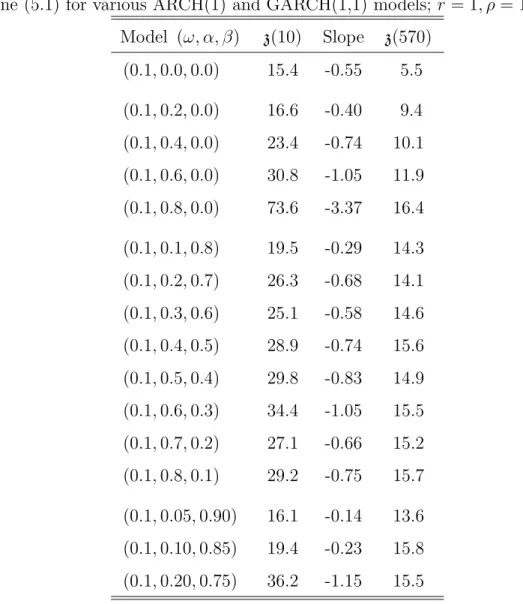
Unfortunately, the critical values depend on the parameters of the underlying (G)ARCH model (in contrast to the case of local constant approximation). We simulated the critical values for ARCH(1) and GARCH(1,1) models with differ-ent values of underlying parameters; see Table 2 for critical values corresponding

to r = 1 and ρ = 1 . The adaptive estimation was performed sequentially on

intervals with length ranging from |I0| = 10 to |IK| = 570 observations using a

geometric grid with the initial interval length m0 = 10 and multiplier a = 1.25 ,

Table 2: Critical values zk = z(|Ik|) of the sequential supremum LR test defined

by line (5.1) for various ARCH(1) and GARCH(1,1) models;r = 1, ρ= 1.

Model (ω, α, β) z(10) Slope z(570) (0.1,0.0,0.0) 15.4 -0.55 5.5 (0.1,0.2,0.0) 16.6 -0.40 9.4 (0.1,0.4,0.0) 23.4 -0.74 10.1 (0.1,0.6,0.0) 30.8 -1.05 11.9 (0.1,0.8,0.0) 73.6 -3.37 16.4 (0.1,0.1,0.8) 19.5 -0.29 14.3 (0.1,0.2,0.7) 26.3 -0.68 14.1 (0.1,0.3,0.6) 25.1 -0.58 14.6 (0.1,0.4,0.5) 28.9 -0.74 15.6 (0.1,0.5,0.4) 29.8 -0.83 14.9 (0.1,0.6,0.3) 34.4 -1.05 15.5 (0.1,0.7,0.2) 27.1 -0.66 15.2 (0.1,0.8,0.1) 29.2 -0.75 15.7 (0.1,0.05,0.90) 16.1 -0.14 13.6 (0.1,0.10,0.85) 19.4 -0.23 15.8 (0.1,0.20,0.75) 36.2 -1.15 15.5

Generally, the critical values seem to increase with the values of the ARCH parameter or the sum of the ARCH and GARCH parameters. To deal with the dependence of the critical values on the underlying model parameters, we pro-pose to choose the largest (most conservative) critical values corresponding to any estimated parameter in the analyzed data. For example, if the largest estimated

parameters of GARCH(1,1) are α_b= 0.3 and βb= 0.8 , one should use z(10) = 25.1

and z(570) = 14.6 . The proposed adaptive search procedure is however not overly

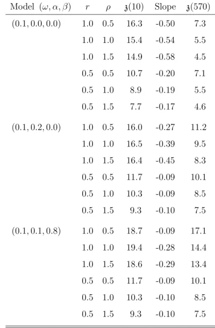
Table 3: Critical values z(|I|) of the sequential supremum LR test defined by line

(5.1) for various ARCH(1) and GARCH(1,1) models and various valuesr and ρ.

Model (ω, α, β) r ρ z(10) Slope z(570) (0.1,0.0,0.0) 1.0 0.5 16.3 -0.50 7.3 1.0 1.0 15.4 -0.54 5.5 1.0 1.5 14.9 -0.58 4.5 0.5 0.5 10.7 -0.20 7.1 0.5 1.0 8.9 -0.19 5.5 0.5 1.5 7.7 -0.17 4.6 (0.1,0.2,0.0) 1.0 0.5 16.0 -0.27 11.2 1.0 1.0 16.5 -0.39 9.5 1.0 1.5 16.4 -0.45 8.3 0.5 0.5 11.7 -0.09 10.1 0.5 1.0 10.3 -0.09 8.5 0.5 1.5 9.3 -0.10 7.5 (0.1,0.1,0.8) 1.0 0.5 18.7 -0.09 17.1 1.0 1.0 19.4 -0.28 14.4 1.0 1.5 18.6 -0.29 13.4 0.5 0.5 11.7 -0.09 10.1 0.5 1.0 10.3 -0.10 8.5 0.5 1.5 9.3 -0.10 7.5

Finally, let us have a look at the influence of the tuning constants r and ρ

in (3.3) on the critical values for several selected models (Table 3). The influence

is significant, but can be classified in the following way. Whereas increasing ρ

generally leads to an overall decrease of critical values (cf. Theorem 3.1), but

primarily for the longer intervals, increasing r leads to an increase of critical values

primarily for the shorter intervals (cf. (3.3)). In simulations and real applications,

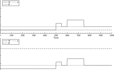
0 100 200 300 400 500 600 700 800 900 1000 0.25 0.50 0.75 1.00 Time Parameter value W B A 0 100 200 300 400 500 600 700 800 900 1000 0.25 0.50 0.75 1.00 Time Parameter value W B A

Figure 2: GARCH(1,1) parameters of low (upper panel) and high (lower panel)

GARCH-effect simulations for t= 1, . . . ,1000.

the performance of the adaptive methods, one can however determine constants

r and ρ in a data-dependent way as described in Section 3.3.2. In the rest of this

section and in Section 6, we use this strategy for a small grid of r ∈ {0.5,1.0}

and ρ ∈ {0.5,1.0,1.5} and find globally the optimal choice of r and ρ; we will

document though that the differences in the average prediction errors (3.7) for

various values of r and ρ are relatively small.

5.2

Simulation study

The main concern of this simulation study is two-fold: (i) to examine how well the proposed estimation method is able to adapt to long stable (time-homogeneous) periods and to less stable periods with more frequent volatility changes, and (ii) to see which adaptively estimated model – local volatility, local ARCH, or local GARCH – performs best in different regimes. To this end, we simulated 100 series

from two change-point GARCH models with a low GARCH effect (ω,0.2,0.1) and

a high GARCH-effect (ω,0.2,0.7) . Changes in constant ω are spread over a time

250 500 750 1000

0.25

0.50

0.75

1.00

Parametric GARCH: Const.

250 500 750 1000 0.25 0.50 0.75 1.00 ARCH parameter 250 500 750 1000 0.25 0.50 0.75 1.00 GARCH parameter 250 500 750 1000 0.25 0.50 0.75 1.00

Adaptive GARCH: Const.

250 500 750 1000 0.25 0.50 0.75 1.00 ARCH parameter 250 500 750 1000 0.25 0.50 0.75 1.00 GARCH parameter

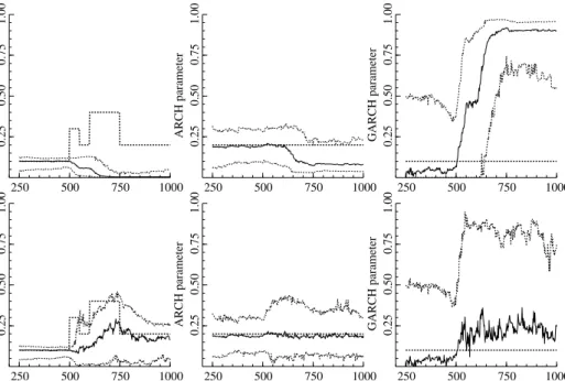
Figure 3: Parameters estimated by the parametric (upper row) and locally

adap-tive (lower row) GARCH methods, t= 250, . . . ,1000.Thick dotted line represents

the true parameter value, solid line is the mean estimate, and the upper and lower dotted lines represent 10% and 90% quantiles of parameter estimates.

(500 days ≈ 2 years) and end (250 days ≈ 1 year) of time series with several

volatility changes between them.

5.2.1 Low GARCH-effect

Let us now discuss simulation results from the low GARCH-effect model. First, we mention the effect of structural changes in time series on the parameter estimation. Later, we compare the performance of all methods in terms of absolute prediction

error (PE), that is, in terms of P EΛ1,H(r, ρ) from (3.7).

Estimating a single parametric model from data containing a change point will necessarily lead to various biases in estimation. For example, Hillebrand (2005)

and Mikosch and Starica (2003) demonstrate that a change in volatility level ω

within a sample drives the GARCH parameter β very close to 1. Therefore, it is

proce-dure, which should try to detect and avoid change points. The parameter estimates

both for parametric and adaptive GARCH at each time point t ∈[250,1000] are

depicted on Figure 3. Let us first observe that, whereas the parametric estimates

are consistent before breaks starting at t = 500 , the GARCH parameter β

be-comes inconsistent and converges to 1 once data contain breaks, t > 500 . The

locally adaptive estimates are similar to parametric ones before the breaks and become rather imprecise after the first change point, but they are not too far from the true value on average and stay consistent (in the sense that the confidence interval covers the true values). The low precision of estimation can be attributed

to rather short intervals used for estimation (cf. Table 1 and Figure 3 fort <500).

Next, we would like to compare the performance of parametric and adaptive

estimation methods by means of absolute prediction error P EΛ1,H in (3.7), where

Λ1(v, v′_{) = |v −v}′_{|; first for the prediction horizon of one day, H = {1}, and}

later for prediction two weeks ahead, H ={1, . . . ,10}. To make the results easier

to decipher, we present in what follows PEs averaged over the past month (21 days). The absolute-PE criterion was also used to determine the optimal values

of parameters r and ρ (jointly for all simulations). The results differ for different

models: r= 0.5, ρ= 0.5 for local constant, r= 0.5, ρ= 1.0 for local ARCH, and

r= 0.5, ρ= 1.5 for local GARCH. Hence, all methods “prefer” in this case flatter

critical-value lines corresponding to r = 0.5 .

Let us now compare the adaptively estimated local constant, local ARCH, and local GARCH models with the parametric GARCH, which is the best performing parametric model in this setup. The average PEs for all methods forecasting one period ahead are presented on Figure 4. First of all, one can notice that all methods

are sensitive to jumps in volatility, especially to the first one at t = 500 : the

parametric ones because they ignore a structural break, the adaptive ones because they use a small amount of data after a structural change. In general, the local

GARCH performs rather similarly to the parametric GARCH for t <625 . After

initial volatility jumps, the local GARCH however outperforms the parametric

250 300 350 400 450 500 550 600 650 700 750 800 850 900 950 1000 0.025 0.050 0.075 0.100 0.125 0.150 0.175 0.200 0.225 0.250 L1 error Time Local constant Local GARCH Local ARCH GARCH

Figure 4: Low GARCH-effect simulations: absolute prediction errors one period ahead averaged over last month for the parametric GARCH and adaptive local

constant, local ARCH, and local GARCH models; t∈[250,1000].

level returns closer to the original level (before t <500 ), the parametric GARCH

is best of all methods for some time, 775< t <850 , until the adaptive estimation

procedure “collects” enough observations for estimation after the last change in volatility. Then the local GARCH (and also local ARCH) become preferable

to the parametric model again, 850 < t. Next, it is interesting to note that

the local ARCH approximation performs almost as well as the GARCH methods

and even outperforms them after several structural breaks, 600 < t < 775 and

850< t <1000 (the only exception to this is the last break at t= 750 ). Finally, the local constant estimation is lacking behind the other two adaptive methods whenever there is a longer time period without a structural break, but keeps up

with them in periods with more frequent volatility changes, 500 < t <650 . All

these observations can be documented also by the absolute PE averaged over the

whole period, t= 250, . . . ,1000 (we refer to it as the global PE from now on): the

smallest PE is achieved by local ARCH (0.075), then by local GARCH (0.079), and the worst result is from local constant (0.094).

250 300 350 400 450 500 550 600 650 700 750 800 850 900 950 1000 0.05 0.10 0.15 0.20 0.25 0.30 0.35 L1 error Time Local constant Local GARCH Local ARCH GARCH

Figure 5: Low GARCH-effect simulations: absolute prediction errors ten periods ahead averaged over last month for the parametric GARCH and adaptive local

constant, local ARCH, and local GARCH models; t∈[250,1000].

Additionally, all models are compared using the forecasting horizon of ten days. Most of the results are the same (e.g., parameter estimates) or similar (e.g., absolute PE) to forecasting one period ahead due to the fact that all models rely on at most one past observation. The absolute PEs averaged over one month are summarized on Figure 5, which reveals that the difference between local constant volatility, local ARCH, and local GARCH models are smaller in this case. As a result, it is interesting to note that: (i) the local constant model becomes a viable alternative to the other methods (it has in fact the smallest global PE 0.107 from all adaptive methods); and (ii) the local ARCH model still outperforms the local GARCH even though the underlying model is GARCH (the global PEs are 0.108

and 0.116, respectively). The GARCH parameter β = 0.1 is however relatively

250 300 350 400 450 500 550 600 650 700 750 800 850 900 950 1000 0.25 0.50 0.75 1.00 1.25 1.50 1.75 L1 error Time Local constant Local GARCH Local ARCH GARCH

Figure 6: High GARCH-effect simulations: absolute prediction errors one period ahead averaged over last month for the parametric GARCH and adaptive local

constant, local ARCH, and local GARCH models; t∈[250,1000].

5.2.2 High GARCH-effect

Let us now discuss the high GARCH-effect model. One would expect much more prevalent behavior of both GARCH models, since the underlying GARCH

pa-rameter is higher and the changes in the volatility level ω are likely to be small

compared to overall volatility fluctuations. Note that the “optimal” choice of

crit-ical values corresponded to the different values of tuning constant r and ρ than

in the case of low GARCH-effect simulations: r= 0.5, ρ= 1.5 for local constant;

r= 0.5, ρ= 1.5 for local ARCH; andr= 1.0, ρ= 0.5 for local GARCH.

Comparing the absolute PEs for one-period-ahead forecast at each time point (Figure 6) indicates that the adaptive and parametric GARCH estimation perform approximately equally well. On the other hand, both the parametric and adap-tively estimated ARCH and constant volatility models are lacking significantly. Unreported results confirm, similarly to the low GARCH-effect simulations, that the differences among method are much smaller once a longer prediction horizon

0 12/91 11/93 10/95 09/97 08/99 07/01 06/03 −0.075 −0.050 −0.025 0.000 0.025 0.050 0.075 Time Returns

Figure 7: The log-returns of DAX series from January, 1990 till December, 2002.

of ten days is used.

6

Applications

The proposed adaptive pointwise estimation method will be now applied to real time series consisting of the log-returns of the DAX and S&P 500 stock indices (Sections 6.1 and 6.2). Similarly to Section 5.2, we summarize the results concern-ing both parametric and adaptive methods by lookconcern-ing at absolute PEs one-day ahead averaged over one month throughout this section. As a benchmark, we use now the parametric GARCH estimated using last two years of data (500 obser-vations). Since we however do not have the underlying volatility process in this case, we approximate the underlying volatility by squared returns. Despite being noisy, this approximation is unbiased and provides usually the correct ranking of methods (Andersen and Bollerslev, 1998).

03/91 12/91 09/92 06/93 03/94 12/94 09/95

1

2

Ratio of L1 errors

Time Local Constant to parametric GARCH

03/91 12/91 09/92 06/93 03/94 12/94 09/95

1

2

Ratio of L1 errors

Time Local ARCH to parametric GARCH

03/91 12/91 09/92 06/93 03/94 12/94 09/95

1

2

Ratio of L1 errors

Time Local GARCH to parametric GARCH

Figure 8: The ratio of the absolute prediction errors of the three pointwise adaptive methods to the parametric GARCH for predictions one period ahead averaged over one month. The DAX index is considered from January, 1992 to March, 1997.

6.1

DAX analysis

Let us now analyze the log-returns of the German stock index DAX from January, 1990 till December, 2002. The whole time series is depicted on Figure 7. In the following analysis, we select several periods interesting for comparing the perfor-mance of parametric and adaptive pointwise estimates since results for the whole period might be hard to decipher at once.

First, let us have a look at the estimation results for years 1991 to 1996. Con-trary to later periods, there are structural breaks practically immediately detected by all adaptive methods (July, 1991 and June, 1992; cf. Stapf and Werner, 2003). In the case of the local GARCH approximation, this differs from less pronounced structural changes discussed later, which are typically detected only with several months delays. One additional break detected by all methods occurs in October

1994. Let us note that parameters r and ρ were r = 0.5, ρ = 1.5 for local

The results for this period are summarized in Figure 8, which depicts the PEs of each adaptive method relative to the PEs of parametric GARCH. First, one can notice that the local constant and local ARCH approximations are optimal at the beginning of the period, where we have less than 500 observations. After the detection of the structural change in June 1991, from July 1991 on, all adaptive methods are shortly worse than the parametric GARCH due to limited amount of data used, but then outperform the parametric GARCH till the next structural break in the second half of 1992. A similar behavior can be observed after the break detected in October 1994, where the local constant and local ARCH models actually outperform both the parametric and adaptive GARCH. In the other parts of the data, the performance of all methods is approximately the same, and even though the adaptive GARCH is overall better than the parametric one, the most interesting fact is that the adaptively estimated local constant and local ARCH models perform equally well. In terms of the global PE, the local constant is best (0.829), followed by the local ARCH (0.844) and local GARCH (0.869). This closely corresponds to our findings in simulation study with low GARCH effect in

Section 5.2. Further, note that even the worst choice of r and ρ results in the

global prediction errors 0.835 and 0.851 for the local constant and local ARCH, respectively. This indicates low sensitivity to the choice of these parameters.

Next, we would like to discuss the estimation results for years 1999 to 2001

(r= 1.0 for all methods now). After the financial markets were hit by the Asian

crisis in 1997 and Russian crisis in 1998, market headed to a more stable state in year 1999. In this case, the adaptive methods detected the structural breaks in the fall of 1997 and 1998. The local GARCH detected them however with more than one-year delay, that is, only in the course of year 1999. The results presented in Figure 9 confirm that the benefits of the adaptive GARCH are practically negligible compared to the parametric GARCH in such a case. On the other hand, the local constant and ARCH methods perform slightly better than both GARCH methods during the first presented year (July 1999 to June 2000). From July 2000, the situation becomes just the opposite and the performance of the GARCH