Predictive Reasoning in Subjective Bayesian Networks

Predictive Reasoning in Subjective Bayesian Networks

Magdalena Ivanovska

and Audun Jøsang

Abstract

Subjective Bayesian networks extend Bayesian networks by substituting the conditional probability distributions with subjective opinions. In that way they enable explicit representation of the uncertainty in the probabilistic information encoded in the network. In this paper we focus on predictive reasoning in subjective Bayesian networks and propose an inference method that is based on the operations of deduction and multiplication of subjective opinions. We demonstrate modelling and inference with subjective Bayesian networks through an example.

1

Introduction

A Bayesian network (BN) is a compact representation of probabilistic information in the form of a directed acyclic graph and probability distributions associated with its nodes. Bayesian network reasoning algorithms provide a way to propagate probabilistic information through the graph, enabling predictive and diagnostic reasoning applicable in risk assessment and decision making. A serious limitation of the Bayesian network reasoning methods is that all the input probabilities must be assigned a precise value in order for the inference algorithms to work and the model to be analysed. This is problematic in many situations where probabilities can not be reliably estimated or are completely missing, while we still want to infer the most accurate conclusions possible. Many different approaches have been proposed for dealing with incomplete Bayesian networks and imprecise probabilistic information in general, like, for example, Bayesian logic (Andersen and Hooker, 1994), credal networks (Cozman, 2000), the probabilistic logics and networks discussed in (Haenni et al., 2011), the logics of likelihood in (Fagin et al., 1990), and imprecise probabilities (Walley, 1991). Conditional reasoning has been an important part of the mentioned theories and has also been analysed in the context of belief theory (Shafer, 1976), (Xu and Smets, 1994).

Subjective Bayesian networks represent second-order uncertainty in BNs, uncertainty

about the probabilities, in the form of subjective opinions. A subjective opinion on a

random variable is a composite representation that includes a specific belief assessment of the random variable done by an expert, based on a test, etc; and a base rate distribution obtained from a background statistics about the knowledge domain. (Ivanovska et al., 2015) provides an introduction to subjective networks and briefly discusses several

possible reasoning approaches. In Bayesian networks, inference is based on evidence

in the form of an observation of some of the variables’ values. In subjective BNs, the evidence itself can in general have the form of a subjective opinion, which provides a

*_{Dept. of Informatics, University of Oslo, Norway}

way of representing soft evidence like, for example, vague observations. In this paper we propose a method for predictive reasoning in subjective BNs which provides a way of propagating subjective evidence from variables to their descendants in the graph. The proposed method combines the deduction operation for subjective opinions described in (Ivanovska et al., 2016) and the operation for multiplication of opinions introduced in (Jøsang and McAnally, 2004).

In Section 2 we introduce subjective BNs providing the necessary preliminaries for Bayesian networks and subjective opinions, but assuming that the reader is familiar with the basics of probability theory. In Section 3 we review the operations of deduction and multiplication of subjective opinions and propose a method for predictive reasoning in subjective BNs. In Section 4 we provide an example to demonstrate the method. In Section 5 we summarize the results of the paper and discuss topics for future work.

2

Subjective Bayesian Networks

Bayesian Networks

A Bayesian network (Pearl, 1988) with n variables is a directed acyclic graph (DAG) with random variablesV ={X₁, . . . ,X_n} as nodes, and a set of conditional probability distributions p(Xi|Pa(Xi)) associated with each node Xi containing one probability

distribution p(X_i|pa(X_i))of X_i for every assignment of values pa(X_i)to its parent nodes Pa(X_i).

If the Markov property holds for the given DAG and the joint distribution p of the

variablesX₁, . . . ,X_n(Every node is conditionally independent of its non-descendant nodes given its parent nodes in the graph,I(X_i,ND(X_i)|Pa(X_i)), then pis determined from the input information in the network as follows:

p(x1, . . . ,xn) = n

∏

i=1

p(xi|pa(Xi)), (1)

where pa(X_i) is the assignment of the parents of X_i that corresponds to the tuple

(x1, . . . ,xn).

The general belief update problem in Bayesian networks is the following: Given

evidence in the form of anobservationof the value of a variableX, to find the probability distribution of another variableY (X andY can also be subsets ofV). There are different belief propagationmethods for solving this problem which make use of the conditional independencies embedded in the graph.

Of importance for our later discussion is the graphical criterion for conditional

independence in Bayesian networks, calledd-separation (see, for example, (Neapolitan,

2003)): For three disjoint sets of nodesX,Y, andZin a DAG, we say thatZ d-separates X

fromY, if every path between a node fromXand a node fromY isblockedbyZ, meaning:

1) there is a node on the path that delivers an arrow and belongs toZ, or 2) there is a node on the path with converging arrows that is neither inZ nor has a descendant that is inZ. IfX andY ared-separated byZ, then they are independent givenZ,I(X,Y|Z).

Subjective Opinions

LetX be a random variable. Asubjective opiniononX (Jøsang, 2008) is a tuple:

where bX :X →[0,1] is a belief mass distribution, uX ∈[0,1] is an uncertainty mass,

and a_X :_X→[0,1] is a base rate distribution of X, satisfying the following additivity constraints:1 uX+

_∑

∑

The beliefs and the uncertainty mass are a result of a specific analysis of the random

variable by applying expert knowledge, experiments, or a personal judgement. bX(x)is

the belief thatX takes the valuexexpressed as a degree in[0,1]. It represents the amount of experimental or analytical evidence in favour ofx. u_X is a single value, representing the degree of uncertainty about the belief analysis. It represents lack of evidence that can be due to lack of knowledge or expertise, or insufficient experimental analysis. The base ratea_X is a prior probability distribution ofX that reflects domain knowledge relevant to the specific analysis, most usually relevant statistical information. For example, a doctor wants to determine whether a patient suffers from depression. Based on examinations and tests, she concludes that the collected evidence is 10% inconclusive, but is still two times more in support of the diagnosis that the patient suffers from depression than of the opposite one. As a result, the doctor assigns 0.6 belief mass to the patient suffering

from depression and 0.3 belief mass to the opposite diagnosis, complemented by 0.1

uncertainty mass. The probability that a random person in the population suffers from depression is 5% and this fact determines the base rates in the doctor’s subjective opinion about the condition of the patient.

A subjective opinion in which uX =0, i.e. an opinion without any uncertainty, is

called adogmatic opinion. Dogmatic opinions correspond to probability distributions. A

dogmatic opinion for which b_X(x) =1, for some x∈_X, is called an absolute opinion.

Absolute opinions correspond to observations. In contrast, an opinion for whichuX =1

(and consequently b_X(x) =0, for every x) is called a vacuous opinion. For a given

multinomial opinion ωX we define its corresponding projected probability distribution

PX :X→[0,1]in the following way:

PX(x) =bX(x) + aX(x)uX . (5)

PX(x) is an estimate for the probability of x which varies from the base rate value, in

the case of complete ignorance (uX =1), to the actual probability in the caseuX =0. In

the correspondence between subjective opinions on a random variable and multinomial Dirichlet model (Walley, 1996) of its distribution given in (Jøsang and McAnally, 2004), the belief massb_X(x)is proportional to the number of observations of x,n(x_i), whileu_X is inversely proportional to the total number of observationsN:

b_X(x_i) = n(xi)

N+s , uX = s

N+s , (6)

wheres is the Dirichlet strength. Then PX corresponds to the mean distribution of the

Dirichlet posterior, ifa_X is the mean of the Dirichlet prior.

Ajoint subjective opinionon variablesX1, . . . ,Xn,n≥2, is a tuple:

ωX1...Xn = (bX1...Xn,uX1...Xn,aX1...Xn), (7)

1_{This definition is for amultinomial subjective opinion. In general, we can definehyper opinions, where}

bX :R(X) =2X\ {X,0}/ , and operate with them through their multinomial projections (see (Ivanovska et al., 2016)).

wherebX1...Xn :X1×. . .×Xn→[0,1]and uX1...Xn ∈[0,1]satisfy the additivity condition

in Eq.(3) anda_X1...Xn is a joint probability distribution of the variablesX₁, . . . ,X_n. Given

two sets of random variablesX andY, aconditional opinion onY given thatX takes the

valuexis a subjective opinion onY defined as a tuple:

ω_Y|x= (b_Y|x,u_Y|x,a_Y|x), (8)

whereb_Y|x:_Y→[0,1]andu_Y|x∈[0,1]satisfy the condition in Eq.(3) anda_Y|x:_Y→[0,1]

is a probability distribution ofY. We use the notationω_Y|X for a set of conditional opinions

onY, one for each value ofX, i.e.:

ω_Y|X ={ω_Y|x|x∈_X}. (9)

Subjective Bayesian Networks

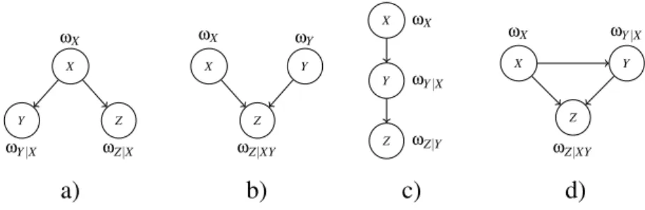
Asubjective Bayesian network (SBN)is a generalization of a classical Bayesian network where each probability distribution p(X|pa(X))is represented with an opinion about it,

ω_X|pa(X) (Fig.1).

The inference problem of opinion updatein an SBN can be formulated as follows:

Given a subjective opinion on an evidence variable X to derive a subjective opinion

on a target variableY.2 This means that, unlike in the case of BNs, we allow for soft

evidence, evidence in the form of a general subjective opinion, not only an absolute one (observation). We denote the derived opinion by ω_YkX. If X is a root node, then ω_YkX

is the marginal opinion onY derived from the network’s input. In the case when X is

not a root node, we assume that by providing an opinion ωX, we ignore the opinion on

X that would be derived from the network’s input, i.e. we “delete” the arrows betweenX

and its parent nodes. A general inference procedure for derivingω_YkX would ideally be

performed in the following steps:

1. The projected probability of the resulting opinion is determined from the projected probabilities of the given opinions using standard BNs reasoning methods.

2. The base rate of the resulting opinion is either given a priori, or determined from

the given ones by Bayesian reasoning or other specified methods.

3. The uncertainty mass and the beliefs are determined by implementing the result of 1. and 2. in Eq.(5), and setting additional constrains that they should satisfy in the specific inference.

While 1. and 2. can be defined in a generic way, it is hard to think of general constrains to be imposed on u_YkX and b_YkX that would apply independently of the position of the evidence and target variable in the graph. That is the reason we apply a piece-wise reasoning strategy, which follows the direction of the arrows in the graph and applies one operation (having its own constraints on the resulting opinion) at a time.

3

Predictive Reasoning in SBNs

Predictive reasoningin Bayesian networks (Korb and Nicholson, 2010) is the reasoning along the direction of the arrows in the DAG in the sense that the target variable

is a descendant of the evidence variables. Determining the marginal probability

X Y Z ωX ωY|X ωZ|X X Y Z ωX ωY ωZ|XY X Y Z ωX ωY|X ωZ|Y X Y Z ωX ωY|X ωZ|XY a) b) c) d)

Figure 1: Three-node subjective Bayesian networks

distribution of a variable can be considered a special case of predictive reasoning

where the set of evidence variables is empty. We present a method for predictive

reasoning in SBNs that combines the subjective logic operations of deduction and multiplication. The deduction operation propagates information from parents to children, while multiplications operation derives the joint opinion from the individual opinions of two or more independent variables. We provide a short review of the deduction and multiplication operation. Then we propose an inference method for singly-connected and a class of multiply-connected networks. The proposed method is an extension of the discussion for predictive reasoning in singly-connected networks provided in (Ivanovska et al., 2016).

Subjective Logic Deduction

Given a set of opinions ω_Y|X and a subjective opinion ωX, the goal of the operation of

deduction is to derive a subjective opinion onY,ωYkX. We denote this by the following

expression:

ω_YkX =ω_Y|X}ωX . (10)

First the projected probability distribution ofω_YkX is determined as follows:3

P(ykX) =

_∑

P(x)P(y|x). (11)

The base rate a_Y is determined by an equation similar to Eq.(11) or supplied from

another source (statistics). It remains to determine the uncertainty and the beliefs of the deduced opinion.

For the belief masses of the deduced opinionω_YkX, we assume the following:

b_ykX ≥min

x∈X

{b_y|x}, (12)

for everyy∈Y, which can be found as aprinciple of plausible reasoningin (Pearl, 1990). Letω_Yk

b

X be the deduced opinion from the vacuous opinion ωbX with a base rate aX. Then u_Yk

b

X is determined as the maximum possible uncertainty mass value under the

conditions imposed by Eq.(12) and Eq.(11) applied to a vacuous opinion. The result is the following expression:

u YkXb =min_y∈ Y ∑xP(y|x)ax−minxby|x ay . (13)

3_{Note that we use simplified notation for the projected probabilities, beliefs, and base rates, for example,}

The uncertainty of the opinion ωYkX deduced from an arbitrary ωX is then determined

as the weighted average of the uncertainty massu

YkXb and the uncertainty masses of the given conditional opinions:

u_YkX =u_Xu

YkXb+

∑

x∈X

b_xu_Y|x. (14)

Eq.(14) is the unique transformation that maps ωbX into u_YkXb, and the corresponding absolute opinions onX intou_Y|x, for x∈_X. Once we have the uncertainty mass of the deduced opinion, the beliefs are easily derived as a consequence, applying Eq.(5).4

Deduction can be generalized for the case whenY has parentsX1. . .Xk, wherek≥2.

Then the input arguments for the deduction operation are: 1) a joint opinion on the parents

ωX1...Xk; and 2) a set of conditional opinionsωY|X1...Xk onY, one for each combination of

values of its parents. While the set of conditional opinionsω_Y|X1...Xk is a part of the input

in a subjective Bayesian network, the joint opinionωX1...Xk would have to be derived. For

this purpose we use the multiplication operation described in the next section.

Subjective Logic Multiplication

Given subjective opinionsωX andωY on two probabilistically independent variables X

andY, the multiplication operation derives an opinionωXY on their joint distribution. We

will denote this by the following expression:

ωXY =ωX·ωY . (15)

Since X and Y are probabilistically independent, the projected probability of the joint

opinion satisfies the following:

P(x,y) =P(x)P(y). (16)

a_XY is either obtained by a similar equation or provided separately. We will assume that

a_XY =a_Xa_Y here. Applying Eq.(5) in Eq.(16), we obtain:

u_XY = bxby+bxuYay+uXaxby+uXuYaxay−bxy

axay

. (17)

We impose the following requirement on the beliefs:

b_xy≥b_xb_y. (18)

For every pair of valuesxandy, the maximum value on the right-hand side of Eq.(17)

is achieved for the smallest allowable value ofb_xy, which is b_xy=b_xb_y. We denote that value withuxy. Applying the latter in Eq.(17), we obtain:

u_xy= bx

ax

u_Y+u_Xby ay

+u_Xu_Y . (19)

We take u_XY to be the minimum of these values, i.e.u_XY =minx,y{uxy}, to assure that

Eq.(18) always holds. This leads to the following expression: uXY =min x,y { bx a_xuY+uX b_y a_y+uXuY}. (20) The beliefsb_xy, forx∈_X andy∈_Y, then follow as a consequence of Eq.(16), Eq.(20), and Eq.(5).

4_{Note that the operation uses only unconditional base rates forY. This is necessary for the condition in}

Eq.(12) to hold for the beliefs ofωYkX. Relaxing on this constraint, we can consider conditional base rates

Reasoning in Three-Node Structures

In this section we analyse the cases of predictive reasoning that appear in the subjective

networks given in Fig.1(a, b, c). The underlying graphs represent the three basic

independence structures.

In thecommon causenetwork given in Fig.1(a), the only case of predictive reasoning

is when we are given a subjective opinion onX and want to derive an opinion onY orZ.

Then only the deduction operation is used in deriving the opinionsωYkX andωZkX from

the opinionωX and the corresponding sets of conditionals given in the network. In this

paper we are generally interested in inference with one evidence and one target variable, but it is worth mentioning that in Fig.1(a), we could easily combine the operations of deduction and multiplication to derive an opinion ω_{Y ZkX} given ωX. First we obtain the

set ω_{Y Z|X} by a series of multiplications: ω_{Y Z|x} =ω_Y|x·ω_Z|x, for every x∈_X, and then

we obtainω_{Y Z}kX applying deduction on ωY Z|X andωX. Multiplication operation can be

applied here because the independence relationI(Y,Z|X)holds.

In thecommon effectnetwork in Fig.1(b), the most natural case of predictive reasoning

is when we are given opinions on the parentsX andY, and want to derive an opinion on

the childZ. Since the variablesX andY in this network are probabilistically independent, we can apply the multiplication operation on the subjective opinionsωX andωY to obtain

the opinionωXY. Then ω_ZkXY =ωZ|XY }ωXY. The case that fits the general inference

problem we are treating here is when we have a single piece of evidence, i.e. evidence

on one of the parents, for exampleωX, and want to derive a subjective opinion onZ. We

obtainω_ZkX in the same way asωZkXY here.

In the chain network in Fig.1(c), predictive reasoning is used when evidence ωX is

given, and opinionω_YkX is derived by deduction. Applying deduction further onω_YkXand ω_Z|Y would complete a predictive reasoning fromX toZderivingωZkX. Alternatively, we

could use two consecutive deductions on the absolute opinions onX, through ω_Y|X and

ω_Z|Y, to derive a set of opinions ω_Z|X, and then use this set to deduce ω_ZkX from ωX.

The first method is preferable though, since it is more direct, involving less operations. If evidence in the form of a subjective opinionωY is available atY, then applying deduction

onωY andωZ|Y we can deriveωZkY. In the latter inference we ignore the input opinion

ωX that is “above” the evidence variableY, and the opinion ωYkX that can be deduced

from it, since we have a new opinion (soft evidence) on the evidence variableY.

Reasoning in Singly-Connected DAGs

A singly-connected DAG is a graph where there is only one path between any two nodes.

Let X be the evidence variable and Y be the target variable in the inference, i.e. we

are given a subjective opinion ωX and want to derive a subjective opinion ωYkX. We

distinguish between the following two cases:

1. The DAG is in the form of atree. This means that every node has only one parent,

so there is an ancestor chain between the evidence and the target: X1→ · · · →Xn

where X₁ =X and X_n =Y. Then the reasoning from the evidence to the target

is a generalization of the reasoning in the chain network in Fig.1(c), i.e. ω_YkX is

obtained byn−1 consecutive deduction operations. IfX is not a root node, then its ancestors in the graph are ignored in the inference.

2. The DAG contains V-structures, i.e. there are nodes that have multiple parents.

Suppose Z is a node on the path between X and Y that has multiple parents.

the d-separation criterion since the only path between each two of them passes

through Z, and Z is a node with converging arrows. This means that we can first

derive subjective opinion on each of the parents of Z separately, and then use the

multiplication operation to findω_Pa(Z)kX, which we further propagate toZ. Because

the graph is singly-connected, the parents ofZ have sets of ancestors that are non-intersecting, hence the deduced opinions on them are derived independently.

Reasoning in Multiply-Connected DAGs

LetX→Y be an arrow in a given DAG. We callX→Y ashortcutif there is another path

in the graph fromX toY containing at least one nodeZother thanX andY. Clearly, all the singly-connected graphs are graphs without shortcuts. The simplest example of a graph

with a shortcut is the three-node connected network given in Fig.1(d). Already in this

network, the inference problem becomes complicated due to absence of the necessary

independencies. In particular, given an opinion ωX as evidence, we can propagate the

evidence toY by applying deduction, but we do not have a way of determining the opinion

ωXY in order to propagate the evidence toZ. Similar problems would appear in any DAG

containing shortcuts.

The simplest example of a multiply-connected DAG that does not contain shortcuts

is the directed diamond structure given in the example in Fig.2(b). We can generalize

the directed diamond to adirected polygon, which is a DAG in the shape of a polygon

with two designated nodes,start Sandfinish F, and two directed paths of arbitrary length (greater than 1) fromStoF.

If the evidence in the directed polygon is at a node E other than the start node S,

then the incoming arrow inE is deleted, and the graph becomes singly-connected. If the

evidence is a subjective opinion on the start nodeS, and the target is not the finishF, we

perform chain reasoning. If the evidence is a subjective opinion on the start nodeS, and

the target node isF, we take the following steps:

• ω_P1|s,ω_P2|s, forP1,P2∈Pa(F), for everys∈S, are determined by chain reasoning. • ω_Pa(F)|s=ωP1|s·ωP2|s, for everys, sinceI(P1,P2|S).

• ω_Pa(F)kS=ω_Pa(F)|S}ωS

• ω_FkS=ω_F|Pa(F)}ωPa(F)kS

If the DAG is consisted of two directed polygons that are connected with the start or finish nodes, and do not have any other nodes in common, then the same reasoning

will still work, since the connection points willd-separate any path from a node in one

polygon to a node in the other. More precisely, we will have one of the following cases: • The polygons are connected at the starts, i.e.S1=S2. Then the predictive inference

problems in them and their solutions are completely disjoint.

• The end of one of the polygons is the start of the other, i.e. F₁ = S₂. Then

any inference problem with an evidence in the “above” polygon and target in the

“below” one is performed by first determining the opinion ω_F1kE by reasoning in

the first polygon, and then propagating it to the target in the second polygon.

• The polygons are connected with the final nodes, i.e. F1 = F2. Then the only

Z D W T S ωZ ωD ω_W|ZD ω_T|D ω_{S|W T} D W T S a) b)

Figure 2: a) A graph of a problematic type, b) The graph of the scholarship example

b_w b_w¯ u_W a_w p_w ωW|d 0.60 0.20 0.20 0.5 0.7 ω_W|d¯ 0.30 0.30 0.40 0.5 0.5 b_t bt¯ uT at pt ωT|d 0.20 0.10 0.70 0.20 0.34 ω_T|d¯ 0.05 0.85 0.10 0.20 0.07

Figure 3: Conditional opinions onW andT given the values ofD

is provided by deducing opinions on the parents of the target node first (which will be a deduction from the new opinion on the evidence node, for the group of parents that are in the same polygon as the evidence node, or a deduction from the opinion on the root (start) node, for the group of parents that are not in the same polygon as the evidence node). Then, the deduced opinions on the two (independent) groups of parents are multiplied and propagated to the target by deduction.

The case of more than two polygons connected in the above described way is dealt with in a similar way. Similar methods apply in a graph structure obtained by connecting a singly-connected graph at one of the end nodes of a directed polygon. Fig.2(a) shows an example of a simple DAG that does not belong to the above discussed categories. The

propagation from D to S in this network would require the set of conditional opinions

ω_W|D, in order to multiply them with the corresponding opinions fromωT|D(I(W,T|D))

and propagate them further to the target, but we do not have a way to determine ω_W|D

from the information provided in the graph.

4

Example

Consider the following situation depicted in Fig.2(b): A student can be granted a college scholarship (S) if she wins a race. Using doping (D) would increase the chances of her winning the race (W) at the same time increasing the chances of her testing positive on the doping test (T) after the race. Another student (we will call her “the analyst”) competing for the same scholarship wants to predict the racers’ chances of receiving the scholarship having an opinion on her use of doping.

We assume all the variables in the example are binary and denote the two states of

a variable X by x and ¯x. The conditional opinions ω_W|D on the influence of doping on

the results in the race are given in the left table of Fig.3. The beliefs and uncertainty in these opinions are subjective estimates of the analyst based on common sense and the current situation, while, in the absence of relevant statistics, the base rates are uniform. The analyst’s opinions about the accuracy of the doping test are given in the right table of Fig.3 and are based on gathered opinions from experts in the laboratory. We can see that the test is very uncertain when there is doping, but still the chances are double for it being accurate rather than inaccurate. In the case of no doping, it will most certainly give

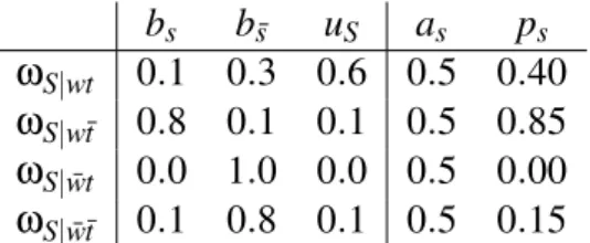
b_s b_s¯ u_S a_s p_s

ω_S|wt 0.1 0.3 0.6 0.5 0.40 ω_S|wt¯ 0.8 0.1 0.1 0.5 0.85

ωS|wt¯ 0.0 1.0 0.0 0.5 0.00

ω_S|w¯t¯ 0.1 0.8 0.1 0.5 0.15

Figure 4: Conditional opinions onSgivenW andT

bwt bwt¯ bwt¯ bw¯t¯ uW T ω_{W T|d} 0.1935 0.2840 0.0575 0.0200 0.4450 ω_{W T|d}¯ 0.0150 0.3850 0.0150 0.3850 0.2000 a_{W T} 0.1000 0.4000 0.1000 0.4000 p_{W T|d} 0.2380 0.4620 0.1020 0.1980 p_{W T|d}¯ 0.0350 0.4650 0.0350 0.4650

Figure 5: Conditional opinions on(W,T)givenD

the correct results, with small chances of giving false positive result based on presence of similar substances. Statistically, the test has shown positive in 20% of the cases.

Granting the scholarship is not completely guaranteed by winning the race and testing negatively on the doping test, it is also based on availability and competition. Also, there is a little chance that the committee decides to grant the scholarship to the winner in case the test shows positive. On the other hand, it can happen that the racer in question does not win the race, but shows dedication and is clean on the test, and obtains the scholarship. The only deterministic case is when the racer does not win and tests positive on the doping test, which results in not obtaining the scholarship. The corresponding opinions are given in Fig.4. The base rate is non-informative.

Assume the analyst has a subjective opinion on the racer taking doping or not given by

ωD= (bD,uD,aD), wherebD= (0.40,0.10),uD=0.50, andad=a_d¯=0.50 and resulting

p_d=0.65. Based on that, she wants to derive a subjective opinion on the racer winning

the scholarship, the opinionω_SkD. Following the procedure described in Section 3, we

first derive the opinions in the set ω_{W T}|D by multiplication: ωW T|d =ωW|d·ωT|d. The

results are presented in Fig.5. Then we apply deduction to obtainω_{W TkD}fromω_{W T|D}and ωD. At the end we apply one more deduction to obtainωSkDfromωS|W T andωW TkD. The

results of these deductions are given in Fig.6.

The resulting opinion suggests belief that is slightly in favor of the racer not winning the scholarship, but we can clearly see that there is a significant amount of uncertainty in this opinion. We can imagine that operating with probabilities only, i.e. excluding the uncertainty factor, is comparable with operating with the projected probabilities here. In this example, it would give the same impression about not obtaining being more probable than obtaining the scholarship, but the uncertainty in this fact (that could be anything from

bwt bwt¯ bwt¯ bw¯t¯ uW T ω_{W TkD} 0.125 0.294 0.036 0.240 0.305 a_{W T} 0.100 0.400 0.100 0.400 p_{W TkD} 0.155 0.416 0.067 0.362 bs bs¯ uS ω_SkD 0.272 0.331 0.397 a_S 0.500 0.500 p_SkD 0.470 0.530

0 to 1) would be ignored.

5

Conclusions and Future Work

In dealing with uncertain probabilistic information, we usually operate with probability estimates where the nature and the amount of evidence they are based on is rarely explicit. The advantage of reasoning with subjective opinions is that it deals with beliefs, uncertainty about them, and prior statistical information at the same time. In that way it enables control over more complex information, returning a more accurate portrait of the modelled situation. The projected probability of a subjective opinion is an estimate for the unknown probability distribution, in which the prior information acts as a backup for the beliefs as much as it is needed (depending on the uncertainty mass).

Subjective Bayesian networks are “uncertain” Bayesian networks whose local modes are subjective opinions instead of probability distributions. In view of the Dirichlet representaton of subjective opinions, SBNs can be seen as credal networks in a hierarchical form (Antonucci et al., 2014), where the hierarchical credal sets(K(X),π)

that correspond to the local conditional distributions are such that K(X) consists of all

the possible distributions of X, and π is a Dirichlet density function over K(X) with

parameters determined by the elements of the subjective opinions. Evidence in SBNs in general takes the form of subjective opinions on some of the network’s variables, which enables reasoning over partial observations or soft evidence in SBNs. This is, in a sense, a generalization of Jeffrey’s updating (Jeffrey, 1983) (where evidence takes the form of a new probability distribution over some of the variables) since subjective opinions are generalization of probability distributions.

We proposed a method for predictive reasoning in SBNs with singly-connected DAGs and multiply-connected DAGs of certain types. The proposed method combines the use of deduction and multiplication operation along the paths from the evidence to the target variable in a way that minimizes the number of applied operations in order to provide a better approximation of the ground truth. The probabilistic inference in BNs, and in particular inferring the marginal probabilities of the nodes, is proven to be NP-hard (Cooper, 1990). Since BNs can be considered as SBNs in which all the subjective opinions are dogmatic (all the uncertainty masses are zero), the problem of determining the marginal probabilities in BNs reduces to a predictive reasoning problem in SBNs and we can conclude that the latter is NP-hard as well.

In future work we want to extend the method to be able to do predictive reasoning in any type of DAGs. Also, evaluation of the procedure as well as a comparison with methods for opinion update based on the Dirichlet representation of subjective opinions (Kaplan and Ivanovska, 2016) will be a part of future work. We are currently working on developing general inference methods for opinion update in SBNs, which will apply to inference problems with any position of the evidence and target variable in the graph, and also to multiple evidence and target variables. In addition to predictive reasoning, this will open the possibilities for diagnostic and combined reasoning.

References

K. A. Andersen and J. N. Hooker. Bayesian logic. Decis. Support Syst., 11(2):191–210,

1994.

Sets. InInformation Processing and Management of Uncertainty in Knowledge-Based Systems, IPMU 2014, pages 456–465, 2014.

G. Cooper. The Computational Complexity of Probabilistic Inference Using Bayesian

Belief Networks. Artificial Intelligence, 42(2):393 – 405, 1990.

F. G. Cozman. Credal networks. Artificial Intelligence, 120(2):199–233, 2000.

R. Fagin, J. Y. Halpern, and N. Megiddo. A Logic for Reasoning about Probabilities. Information and Computation, 87:78–128, 1990.

R. Haenni, J.-W. Romeijn, G. Wheeler, and J. Andrews. Probabilistic Logic and

Probabilistic Networks. Synthese Library, 350(8), 2011.

M. Ivanovska, A. Jøsang, L. Kaplan, and F. Sambo. Subjective Networks: Perspectives

and Challenges. Fourth International Workshop of Graph Structures for Knowledge

Representation and Reasoning (GKR2015), pages 107–124, 2015.

M. Ivanovska, A. Jøsang, and F. Sambo. Bayesian Deduction with Subjective Opinions. In 15th International Conference on Principles of Knowledge Representation and Reasoning (KR 2016), pages 484–493. AAAI press, 2016.

R. Jeffrey. The Logic of Decision. McGraw-Hill, 2nd edition Univ. of Chicago press,

1983.

A. Jøsang. Conditional Reasoning with Subjective Logic. Journal of Multiple-Valued

Logic and Soft Computing, 15(1):5–38, 2008.

A. Jøsang and D. McAnally. Multiplication and Comultiplication of Beliefs.International

Journal of Approximate Reasoning, 38(1):19–51, 2004.

L. Kaplan and M. Ivanovska. Efficient Subjective Bayesian Network Belief Propagation

for Trees. In19th International Conference on Information Fusion (FUSION 2016), to

appear, 2016.

K. Korb and A. Nicholson. Bayesian Artificial Intelligence, Second Edition. CRC Press,

2010.

R. E. Neapolitan. Learning Bayesian Networks. Prentice Hall, 2003.

J. Pearl. Probabilistic Reasoning in Intelligent Systems: Networks of Plausible Inference. Morgan Kaufmann, 1988.

J. Pearl. Reasoning with Belief Functions: An Analysis of Compatibility. International

Journal of Approximate Reasoning, 4(6):363–389, 1990.

G. Shafer. A Mathematical Theory of Evidence. Princeton University Press, 1976.

P. Walley. Statistical Reasoning with Imprecise Probabilities. Chapman and Hall, 1991.

P. Walley. Inferences from Multinomial Data: Learning about a Bag of Marbles. Journal

of the Royal Statistical Society, 58(1):3–57, 1996.

H. Xu and P. Smets. Evidential Reasoning with Conditional Belief Functions. In

D. Heckerman et al., editors, Proceedings of Uncertainty in Artificial Intelligence