ROBUST MODEL-FREE VARIABLE SCREENING, DOUBLE-PARALLEL MONTE CARLO AND AVERAGE BAYESIAN INFORMATION CRITERION
A Dissertation by
JINGNAN XUE
Submitted to the Office of Graduate and Professional Studies of Texas A&M University
in partial fulfillment of the requirements for the degree of DOCTOR OF PHILOSOPHY
Chair of Committee, Samiran Sinha Committee Members, Bani Mallick
Anirban Bhattacharya Jianxin Zhou
Head of Department, Valen Johnson
August 2017
Major Subject: Statistics
ABSTRACT
Big data analysis and high dimensional data analysis are two popular and chal-lenging topics in current statistical research. They bring us a lot of opportunities as well as many challenges. For big data, traditional methods are generally not efficient enough to handle them, from both time perspective and space perspective. For high dimensional data, most traditional methods can’t be implemented, let alone maintain their desirable properties, such as consistency.
In this disseration, three new strategies are proposed to solve these issues. HZ-SIS is a robust model-free variable screening method and possesses sure screening property under the ultrahigh-dimensional setting. It works based on the nonpara-normal transformation and Henze-Zirkler’s test. The numerical results indicate that, compared to the existing methods, the proposed method is more robust to the data generated from heavy-tailed distributions and/or complex models with interaction variables.
Double Parallel Monte Carlo is a simple, practical and efficient MCMC algorithm for Bayesian analysis of big data. The proposed algorithm suggests to divide the big dataset into some smaller subsets and provides a simple method to aggregate the subset posteriors to approximate the full data posterior. To further speed up com-putation, the proposed algorithm employs the population stochastic approximation Monte Carlo (Pop-SAMC) algorithm, a parallel MCMC algorithm, to simulate from each subset posterior. Since the proposed algorithm consists of two levels of par-allel, data parallel and simulation parpar-allel, it is coined as “Double Parallel Monte Carlo”. The validity of the proposed algorithm is justified both mathematically and numerically.
Average Bayesian Information Criterion (ABIC) and its high-dimensional variant Average Extended Bayesian Information Criterion (AEBIC) led to an innovative way to use posterior samples to conduct model selection. The consistency of thismethodis established for the high-dimensional generalized linear model under some sparsity and regularity conditions. The numerical results also indicate that, when the sample size is large enough, this method can accurately select the smallest truemodelwith high probability.
ACKNOWLEDGMENTS
First and foremost I would like to express my sincerest gratitude to my advisor, Dr. Faming Liang for his excellent guidance, systematic mentoring, and constant support throughout my entire doctoral study. I’m very lucky to have him as my advisor. Without his help, I would not be able to finish this dissertation. His continuous passion in research and deep understanding of statistical methodology also let me know what properties one should possess to achieve success in academia. My gratitude also goes to my committee chair, Dr. Samiran Sinha, for assisting me to handle documents with patience, and other committee members, Dr. Bani Mallick, Dr. Anirban Battacharya, Dr. Jianxin Zhou for generously giving insightful comments and suggestions to improve my dissertation work. I’m very honored to have them on my Ph.D. advisory committee.
I would also like to express my thanks to Dr. Michael Longnecker for his constant help ever since I entered the department. As the associate department head, he is extremely caring and nice to every graduate student. I’m also thankful to Dr. Jianhua Huang, Dr. Jeffery Hart, Dr. Willa Chen, Dr. Ursula Mueller, Dr. Valen Johnson, Dr. Mohsen Pourahmadi, Dr. Huiyan Sang, Dr. Suhasini Subba Rao, Dr Edward Jones and Dr. Raymond Carroll. I really learned a lot from their courses.
Last but not least, I would like to thank my parents for providing me uncondi-tional support and all my friends for making my past five years colorful and memo-rable. I’ll cherish this for the rest of my life.
CONTRIBUTORS AND FUNDING SOURCES
Contributors
This work was supervised by Professor Faming Liang and a dissertation commit-tee consisting of Professor Samiran Sinha (chair), Professor Bani Mallick, Professor Anirban Bhattacharya from the Department of Statistics and Professor Jianxin Zhou from the Department of Mathematics.
All work conducted for the dissertation was completed by the student indepen-dently.
Funding Sources
Graduate study was supported by a fellowship from Texas A&M University and in part by the NSF grants DMS-1545202 and DMS/NIGMS R01-GM117597.
TABLE OF CONTENTS
Page
ABSTRACT . . . ii
ACKNOWLEDGMENTS . . . iv
CONTRIBUTORS AND FUNDING SOURCES . . . v
TABLE OF CONTENTS . . . vi
LIST OF FIGURES . . . viii
LIST OF TABLES . . . ix
1. INTRODUCTION . . . 1
1.1 High Dimensional Data . . . 1
1.2 Big Data . . . 3
1.3 Dissertation Structure . . . 5
2. ROBUST MODEL-FREE FEATURE SCREENING FOR ULTRAHIGH DIMENSIONAL DATA . . . 6
2.1 Introduction . . . 6
2.2 Robust Feature Screening . . . 8
2.2.1 The Method . . . 8
2.2.2 Theoretical Properties . . . 12
2.3 Simulation Studies . . . 14
2.3.1 An Additive Model Example . . . 15
2.3.2 A Model with Interaction Variables . . . 17
2.3.3 A Complex Model with More Interaction Variables . . . 19
2.4 Screening of Anticancer Drug Response Genes . . . 20
3. DOUBLE-PARALLEL MONTE CARLO FOR BAYESIAN ANALYSIS OF BIG DATA . . . 24
3.1 Introduction . . . 24
3.2 Subset Posterior Aggregation . . . 26
3.3.1 Pop-SAMC Algorithm and Its OpenMP Implementation . . . 30
3.3.2 Double Parallel Monte Carlo . . . 33
3.4 Simulation Study . . . 34
3.4.1 Logistic Regression . . . 34
3.4.2 Linear Regression with Unknown Variance . . . 35
3.5 A Big Data Example . . . 38
4. AVERAGE BAYESIAN INFORMATION CRITERION AND ITS APPLI-CATION TO HIGH DIMENSIONAL GENERALIZED LINEAR MODEL 42 4.1 Introduction . . . 42
4.2 Average Extended Bayesian Information Criterion . . . 46
4.3 Consistency . . . 52
4.4 Simulation . . . 54
4.4.1 Low Dimensional Logistic Regression . . . 55
4.4.2 Low Dimensional Linear Regression . . . 57
4.4.3 High Dimensional Logistic Regression . . . 58
4.4.4 High Dimensional Linear Regression . . . 59
4.5 Real Data Example . . . 60
5. SUMMARY AND DISCUSSIONS . . . 63
REFERENCES . . . 66
APPENDIX A. SUPPLEMENTARY MATERIALS FOR CHAPTER 2 . . . . 74
A.1 Proof of Lemma 2.1 . . . 74
APPENDIX B. SUPPLEMENTARY MATERIALS FOR CHAPTER 3 . . . . 83
B.1 Proof of Theorem 3.1 . . . 83
APPENDIX C. SUPPLEMENTARY MATERIALS FOR CHAPTER 4 . . . . 86
C.1 A Useful Lemma . . . 86
C.2 Proof of Theorem 4.1 . . . 97
LIST OF FIGURES
FIGURE Page
2.1 Histograms of the screening indices of different methods for the addi-tive model example with the predictors generated from the distribu-tion t(4). . . 17 2.2 Scatter plots of the transformed response variable Tey(Y) versus the
transformed predictors Te1(X1),Te50(X50) and Te100(X100) . . . 19
3.1 Binned kernel posterior density estimates for the parameters of a lo-gistic regression. The true parameter θ∗ = (1,−1)T (black dot). . . . 36 3.2 QQ-plots for the normal regression example. The top, middle and
bottom panels are for the double parallel, WASP and consensus Monte Carlo, respectively. . . 38
LIST OF TABLES
TABLE Page
2.1 Simulation results for the additive model example. For MSD, we re-port the median with its associated interquartile range (IQR) in the parentheses. . . 16 2.2 Results for the model with interaction variables. For MSD, we
re-port the median with its associated interquartile range (IQR) in the parentheses. . . 18 2.3 Results for the complex model with more interaction variables. For
MSD, we report the median with its associated interquartile range (IQR) in the parentheses. . . 20 2.4 Top 10 genes selected for the drug topotecan by different methods. . . 22 2.5 Top 10 genes selected for the drug 17-AAG by different methods. . . 23 3.1 Comparison of computational time (wall clock time) and parameter
estimation for the MiniBooNE particle data set. . . 41 4.1 Simulation results of AIC,BIC,DIC and ABIC for the low dimensional
logistic regression . . . 56 4.2 Simulation results of AIC,BIC,DIC and ABIC for the low dimensional
linear regression . . . 57 4.3 Simulation results of EBIC and AEBIC for the high dimensional
lo-gistic regression . . . 58 4.4 Simulation results of EBIC and AEBIC for the high dimensional linear
regression . . . 60 4.5 AEBIC and 1-CVMR for the top 10 models with highest AEBIC . . . 61 4.6 Top 10 genes in Chen and Chen (2012) and their corresponding
1. INTRODUCTION
Big data and High dimensional data are two popular and challenging topics in current statisticial research. Both have attracted lots of attention and lead to nu-merous innovative methods. This dissertation contributes three new approaches, the first and the third one can be used to deal with high dimensional data, and the second one is developed for big data analysis.
1.1 High Dimensional Data
In statistics, high-dimensional data usually refers to the data whose dimension p is larger than the sample size n and ultrahigh-dimensional data usually refers to the data where p grows exponentially withn, that is, p=O(nα).
In recent years, high dimensional data analysis has become more frequent and im-portant in diverse fields of our daily life, such as genomics, microarrays, proteomics, brain images, climatology, geology, neurology, health science,economics, finance and machine learning (Fan and Lv, 2010). For example, in genowide association stud-ies between genotypes and phenotypes, millions of SNPs are potential covariates; in disease classfication using microarray or proteomics data, thousands of expression profiles are potential predictors; in biomedical and clinical studies, a large number of magnetic resonance images (MRI) and functional MRI data are collected for each subject. Moreover, when interaction are considered, the dimensionality will grow more quickly. These massive amounts of high dimensional data have undoubtedly brought many opportunities for scientific development. However, at the same time, they have also significantly challenged traditional statistical theory (Fan and Li, 2007; Johnstone and Titterington, 2009).
even in the low dimensional case, the notorious collinearity will sometimes cause lots of trouble, and force us to use PCA or any other techniques to solve it. In the high dimensional setting, this problem becomes worser and usually makes us to overfit the data and select wrong models, since any variable can be well approximated or even replaced by a combination of spurious variables. Besides, under the high dimensional setting, some traditional methods can’t even be implemented. For example, in gaus-sian graphical models (GGM), the sample covariance matrix is singular when p > n, thus we can no longer directly estimate the concentration matrix and use it to learn the graph. (Liang et al., 2015) Noise accumulation in high dimensional prediction has been recongnized as another challenge. In fact, in supervised learning problems, prediction using all features can be as bad as random guess. Therefore, variable selection is fundamentally important to high dimensional data analysis, for both re-gression and classification. To overcome these challenges and make high dimensional statistical inference possible, we usually impose the so called sparsity condition. For example, in supervised learning, that means most of the features are irrelevant with the response variable; in Gaussian Graphical Models, that means only few edges truly exist. With sparsity assumption and specific methods, variable selection is able to possess the consistency property and can be implemented to improve the model interpretability and prediction accuracy.
In the past decades, numerous innovative methods have been proposed to deal with high dimensional data. The frequentist methods are usually regularition-based, imposing a penalty on the likelihood function to enforce sparsity. For example, Tib-shirani (1996) employs a l1-penalty, Zou and Hastie (2005) employs a combination of l1 and l2 penalties, Fan and Li (2001) employs a smoothly clipped absolute devia-tion penalty, Zhang (2010) employes minimax concave penalty and Song and Liang (2015) employes a reverse l1 penalty. The Bayesian methods usually employ
appro-priate prior distributions to enforce sparsity, such as the non-local priors (Johnson and Rossell, 2012), the priors used in EBIC (Liang et al., 2013; Chen and Chen, 2008, 2012), etc.
In this disseration, we contribute two more methods. In Chapter 2, we’ll intro-duce a robust model-free variable screening method. It is well known that variable screening can reduce the dimension of feature space to a moderate scale while keeping all relevant features. Thereby it can act as a preliminary step ahead of variable se-lection. Compared to the previous proposed model-free variable screening methods, which more or less require some additional assumptions and are not robust to non-regular data, our method only needs few assumptions to guarantee its sure screening property under ultrahigh-dimensional setting, and is more robust to the heavy-tailed data and data with interaction effects. In Chapter 4, we’ll describe a new informa-tion criterion, ABIC and its high dimensional variant AEBIC. To our knowledge, AEBIC is the first information criterion that use information from posterior samples and possess model selection consistency.
1.2 Big Data
Big data often refers to the data whose the sample size is too large such that it can not be processed and stored on a single computer.
Nowadays, we are entering the era of Big data, thanks to the technology develop-ment and information explosion. Big data can be found almost everywhere around our life. For example, Walmart handles more than 1 million customer transactions every hour, which are imported into databases estimated to contain more than 2.5 petabytes of data - the equivalent of 167 times the information contained in all the books in the US Library of Congress; Amazon.com handles millions of back-end operations every day, as well as queries from more than half a million third-party
sellers; Windermere Real Estate uses anonymous GPS signals from nearly 100 mil-lion drivers to help new home buyers determine their typical drive times to and from work throughout various times of the day.
Big data brings opportunities to modern society. It helps us discover many new findings which are not possible with small-scale data. At the same time, the massive sample size also brings unique challenges to computational and statistical research. (Fan et al., 2014) They mainly come from two aspects. One is on data storage and the other is on computational time. Although hardware is being upgraded in an unprecedented speed to enlarge storage memory and decrease computational time, more efficient algorithms are still highly required to solve these challenges.
Thanks to the advent of parallel computing, a large number of efficient approaches have now been proposed to deal with Big data. For example, it is well known that when making Bayesian inference for big data, traditional MCMC algorithms are generally not efficient enough. Therefore, people propose to divide the large dataset into a number of smaller subsets, and then conduct the Bayesian analysis for each subset separately. Finally, the posterior samples generated for each subset are aggregated in some way such that a correct inference can be made for the full data posterior. Several algorithms have been developed to address the issue of subset posterior aggregation, such as Scott et al. (2016); Neiswanger et al. (2013); Wang and Dunson (2013); Minsker et al. (2014);?); Srivastava et al. (2015)
In Chapter 3, we introduce a new method for aggregating subset posterior sam-ples. The new method is surprisingly simple, which is to first simulate from some modified subset posteriors, for which the log-likelihood functions are appropriately scaled according to their sample size, and then recenter the subset posterior samples to their global mean. In order to further speed up computation, we suggest to use the Pop-SAMC algorithm (Song et al., 2014), rather than traditional single chain
MCMC algorithms, to draw samples from each subset posterior. Since the proposed method consists of two levels of parallel, data parallel and simulation parallel, it is coined as "double parallel” Monte Carlo.
1.3 Dissertation Structure
The rest of the dissertation is organized as follows. Chapter 2 introduces a ro-bust model-free variable screening method to deal with ultra-high dimensional data. Chapter 3 develops the Double-Parallel Monte Carlo algorithm for Bayesian analy-isis of big data. Chapter 4 is dedicated to the Average Bayesian Information Crite-rion(ABIC) and its high-dimensional variant Average Extended Bayesian Information Criterion(AEBIC). Chapter 5 gives a summary of this dissertation and points out some directions for future research. The technical details and supplementary results are included in the Appendix.
2. ROBUST MODEL-FREE FEATURE SCREENING FOR ULTRAHIGH DIMENSIONAL DATA
2.1 Introduction
Variable selection plays an important role in high-dimensional data analysis. However, under the ultrahigh-dimensional setting, where the number of covariates may grow at an exponential rate of sample size, current variable selection methods may not work well due to the simultaneous challenges of computational expediency, statistical accuracy, and algorithmic stability (Fanet al., 2009). A practical approach is using a screening procedure to reduce the dimension of feature space to a moderate scale, and then implementing variable selection methods on the reduced dataset. To pursue this approach, Fan and Lv (2008) proposed the sure independence screening (SIS) method for linear regression, which screens predictors by ranking their Pearson correlations with the response variable. They established the sure screening property, that is, all active predictors can be selected with probability approaching one as the sample size increases to infinity. Fan and Song (2010) extended SIS to generalized linear models, which screens features by ranking the maximum marginal likelihood estimators. As for nonlinear feature screening, Hall and Miller (2009) suggested poly-nomial transformations of predictors, and Fanet al.(2011) suggested to estimate the nonparametric components marginally using B-splines and then screen the features by ranking the magnitude of nonparametric components.
All the above methods require the specification of a particular model structure. If the underlying model is correctly specified, these methods can perform well. How-ever, if the underlying model is misspecified, their performance may be corrupted. Under the ultrahigh dimensional setting, specifying a correct model is usually an
impossible task, thus the model-free feature screening methods are often appealing. Toward this direction, Zhu et al. (2011) proposed a sure independence ranking and screening (SIRS) method to screen significant features for multi-index models. Li
et al. (2012) proposed a distance correlation sure independence screening (DC-SIS) method, which screens features based on their distance correlations (Székely et al., 2007) with the response variable. It is known that for two random variables, zero dis-tance correlation implies independence. Heet al.(2013) proposed a quantile-adaptive sure independence screening (Qa-SIS) method, which employs spline approximation to model the marginal effects of the predictors at a quantile level and then uses it to screen variables. A particular strength of this method is that it can handle the cen-sored data arising in survival analysis. Recently, Cuiet al.(2015) established a mean variance sure independence screening (MV-SIS) method, where the dependence of two random variables is measured using the mean variance of the conditional distribu-tion funcdistribu-tion. This method is originally proposed for categorical response variables, but can be extended to the problems for which the response variable is continuous via discretization.
Although the model-free variable screening methods avoid the specification of a particular model structure, they are still based on some assumptions for the pre-dictor and response variables, more or less. For example, DC-SIS requires both the predictors and the response variable to satisfy the sub-exponential tail probability uniformly. That is, practically, the response variable and predictors should be uni-formly bounded or follow a multivariate Gaussian distribution. Qa-SIS requires the conditional quantile function’s derivative to satisfy a Lipschitz condition and the conditional density function to be uniformly bounded for each feature.
In this chapter, we introduce a new model-free feature screening method and establish its sure independence screening property under the ultrahigh dimensional
setting. The proposed method works based on the nonparanormal transformation (Liu et al., 2009) and Henze-Zirkler’s test (Henze and Zirkler, 1990). It is to first transform the response variable and each of the predictors to Gaussian random vari-ables using the nonparanormal transformation and then test the dependence between the response variable and the predictors using the Henze-Zirkler’s test. Compared to the existing methods, the proposed method requires fewer assumptions to guarantee its sure independence screening property and thus performs more robustly. Our nu-merical studies indicate that the new method can achieve better performance when the covariates follow a heavy-tailed distribution and when the underlying true model is complex with interaction variables.
The rest of this chapter is organized as follows. In Section 2.2, we describe the proposed method and establish its sure independence screening property. In Section 2.3, we conduct simulation studies to evaluate the finite sample performance of the proposed method along with comparisons with the existing methods. In Section 2.4, we apply the proposed method to screening of anticancer drug response related genes.
2.2 Robust Feature Screening 2.2.1 The Method
LetY denote the continuous response variable, letX = (X1, . . . , Xp)denote the continuous covariates, letndenote the sample size of the data, and letf(y|x)denote the conditional distribution ofY givenX. Under the ultrahigh-dimensional setting, where p=O(exp(nτ))for some τ >0, we generally assume that only few predictors are relevant to the response variable, although the covariate dimension p greatly exceeds the sample size n. Without specifying a parametric form for the regression
model, we define the sets of active predictors and inactive predictors as follows:
D ={k:f(y|x)functionally depends on Xk},
I ={k:f(y|x)does not functionally depends on Xk}.
Directly identifying the active predictor setD is sometimes difficult or even impossi-ble under the ultrahigh-dimensional setting. Therefore, people proposed to first find a larger set with a moderate size including all elements in D, then apply variable selection techniques on this larger set to accurately identify D. Note that if f(y|x) functionally depends onXk, thenY andXkare usually marginally dependent as well, therefore we can select the marginally dependent predictors to construct the larger set, which is usually referred to as independence screening. In fact, under the partial orthogonality condition (Fan and Song, 2010; Huanget al., 2008), that is,{xi, i∈D} is independent of {xj, j ∈I}, we can further show that f(y|x)functionally depends on xk if and only if Y and Xk are marginally dependent.
To implement independence screening, we need to find a metric to measure the marginal dependence between each predictorXkand the response variableY. Several metrics have already been proposed, see e.g., Zhu et al.(2011), Cui et al. (2015), Li
et al. (2012), and He et al. (2013). In this chapter, we propose a new one with the basic idea described as follows. Let Fy(·) denote the CDF of the response variable
Y, and Fk(·)denote the CDF of the kth predictorXk. Consider the nonparanormal transformation (Liu et al., 2009)
Ty(Y) = Φ−1(Fy(Y)), Tk(Xk) = Φ−1(Fk(Xk)), k= 1, . . . , p, (2.1)
nonparanormal transformation implemented here is slightly different with the original one because we don’t need the mean and variance correction step. In addition, Liu
et al.(2009) imposed nonparanormal transformation on nonparanormal distributions, but here we just use this transformation on common random vectors.
It is easy to see thatY is independent ofXk if and only if(Ty(Y), Tk(Xk))forms a bivariate random vector following the distribution N2(0,I2), where I2 denotes the 2×2 identity matrix. The latter can be tested using a multivariate normality test, e.g., Henze-Zirkler’s test (Henze and Zirkler, 1990), with the known covariance structure. If (Ty(Y), Tk(Xk)) does not follow the distribution N2(0,I2), then the Henze-Zirkler’s test statistic tends to take a large value. In practice, sinceFyandFk’s are usually unknown, we can use the estimated nonparanormal transformation in Liu
et al. (2009). The estimated nonparanormal transformation has been implemented
in the R package huge.
In summary, the proposed method consists of the following steps:
1. Transform all variables, including the response variable and predictors, to stan-dard Gaussian random variables by the estimated nonparanormal transforma-tion. Let’s take the response variable as example, let
e
Ty(yi) = Φ−1(Fey(yi)), i= 1, . . . , n,
whereyi denotes the ith observation ofY, Fey is the truncated empirical
distri-bution of Y given by e Fy(t) = δn :Fby(t)< δn, b Fy(t) :δn≤Fby(t)≤1−δn, 1−δn :Fby(t)>1−δn,
b
Fy(t)≡ 1nPi=1n 1{yi≤t} is the empirical distribution of Y, and the default
trun-cation parameter δn = 14n−1/4(πlogn)−1/2.
2. For each predictorXk, calculate the Henze-Zirkler test statistic
e ωk∗ = 1 n2 n X i=1 n X j=1 e−β 2 2 dij− 2 n(1 +β2) n X i=1 e− β2 2(1+β2)di + 1 1 + 2β2, (2.2) where β is the smoothing parameter and its optimal value is (1.25n)1/6/√2, corresponding to the optimal bandwidth for a nonparametric kernel density estimator with Gaussian kernel (Henze and Zirkler, 1990). In addition, dij = (Tek(xki)−Tek(xkj))2+ (Tey(yi)−Tey(yj))2,di =Tek2(xki) +Tey2(yi), and Tek(xki)and
e
Ty(yi) denote the ith realization of Tek(Xk) and Tey(Y), respectively. 3. Select a set of important predictors with large value of ωek∗, i.e., set
b
D={k :eω∗k> cn−κ,for 1≤k ≤p},
where cand κ are predetermined threshold values.
Sincecandκare usually difficult to determine, we follow the other feature screen-ing methods to set the size ofDb to be [n/log(n)], where [z] denotes the integer part
ofz. Since the proposed method employes the Henze-Zirkler test statistic to measure the dependence between the transformed response variable and predictors, we call it the Henze-Zirkler sure independence screening method or HZ-SIS for short.
2.2.2 Theoretical Properties
To study the theoretical properties of the HZ-SIS method, we first describe how the HZ-test statistic ωe∗k in (2.2) is derived. Define
ωk = Z R2 φk(t)−exp(−1 2t 0 t) 2 ϕβ(t)dt, k = 1,2, . . . , p,
where φk(t) is the characteristic function of (Φ−1(Fk(Xk)),Φ−1(Fy(Y))), and ϕβ(t) is the density function of N(0, β2I
2). Recall that exp(−12t0t) is the characteristic function of N(0, I2). Therefore,ωk can be viewed as the averaged difference between the characteristic function of the transformed variables and the characteristic func-tion of N(0, I2). It is easy to verify that ωk equals zero if and only if Xk and Y are marginally independent.
Given observations {(x1, y1), . . . ,(xn, yn)}, wherexi ={x1i, . . . , xpi} denotes the predictor variables inith observation, we first use the truncated empirical distribution to estimate the CDF for each variable. In order to estimate ωk, we re-express it in the following form (Henze and Zirkler, 1990) by some algebra:
ωk =E n e−β 2 2 [(Φ −1(F k(Xk))−Φ−1(Fk(Xk0))) 2+(Φ−1(F y(Y))−Φ−1(Fy(Y0)))2] − 2 1 +β2e − β2 2(1+β2)(Φ −1(F k(Xk))2+Φ−1(Fy(Y))2) + 1 1 + 2β2 o ,
where (Xk0, Y0) is an independent copy of (Xk, Y). With this representation, ωk can be estimated using a V-statistic, which leads to the HZ-test statistic used in (2.2).
Next, we study the sure screening property of the HZ-SIS method. As mentioned previously, compared to the existing methods, HZ-SIS requires fewer assumptions for its sure screening property. The assumptions are given as follows.
2cn−κ.
C2 The dimension p=O(exp(nτ)) for some constant0≤τ < 1−4κ 3 .
Assumption (C1) can be viewed as a regularity condition for sure screening meth-ods, which assumes that the minimum true signal cannot be too weak to be detectable for a given sample size, although it can gradually diminish to zero as the sample size increases to infinity. A similar assumption has been used in other methods, see e.g., Liet al.(2012) and Cuiet al.(2015). Assumption (C2) allows an exponential growth of the dimension p as a function of the sample size. It is also regular for ultrahigh dimensional methods. To establish the sure screening property for HZ-SIS, the key step is to establish an exponential probability bound for |eω∗k−ωk|. The following lemma presents such an exponential probability bound with the proof given in the Appendix.
Lemma 2.1. If the truncation parameter δn = 4n
m 2 √ 2πmlogn−1, where m = 2 3 − 2κ
3, then there exist positive constants c1 >0 such that
P( max 1≤k≤p|ωe ∗ k−ωk|> cn −κ )≤O pexp{−c1n 1−4κ 3 } , for 1< k≤p.
Here we note that we set m = 1/2 as the default value for the HZ-SIS method and this default value has been used in all examples of this chapter. Based on this lemma, we establish the sure screening property for HZ-SIS in the following theorem. Theorem 2.1. Under conditions (C1) and (C2), we have
Proof. If D * Dˆ, there must exist k0 ∈ D such that eω∗k0 < cn−κ. Recall that
ωk >2cn−κ for allk∈D. Therefore, we have |ωe ∗
k0−ωk0|> cn−κ. This indicates that {D*Db} ⊆ { there existk0 ∈D such that |
e
ωk∗0 −ωk0|> cn−κ}. Consequently,
P(D⊆Db) = 1−P(D*Db)
≥ 1−P(there existk0 ∈D such that |ωek∗0 −ωk0|> cn−κ) ≥ 1−P( max 1≤k≤p|ωe ∗ k−ωk|> cn−κ)≥1−O{pexp{−c1n 1−4κ 3 }} = 1−O{exp{−c1n 1−4κ 3 + log(p)}} = 1−O{exp{−c1n 1−4κ 3 +c2nτ}}= 1−o(1),
which concludes the proof. 2.3 Simulation Studies
In this section, we used three simulated examples to assess the finite sample performance of HZ-SIS, along with comparisons with SIS (Fan and Lv, 2008), DC-SIS (Li et al., 2012), Qa-SIS (He et al., 2013) and MV-SIS (Cui et al., 2015). In addition, NIS (Fanet al., 2011) was implemented for additive model(Example 2.3.1), and the screening step in slice inversion regression for interaction detection (SIRI) was implemented for model with interactions(Example 2.3.2 & 2.3.3). For each example, we generated 100 independent datasets and summarized the performance of the methods on these 100 datasets in a few statistics. These statistics include the minimum size of Db needed to cover all active variables, which is denoted by MSD
for short; and for the given size νn = [n/log(n)] of Db, the proportion of Db covering
a single active predictor Xk (denoted by Pk), and the proportion of Db covering all
active variables (denoted byPa). The reason for choosing the above statistics is that in practice, we usually specify the sizeνnof Db instead of the thresholding valuecn−κ
for feature screening.
2.3.1 An Additive Model Example
This example is adopted from Cuiet al. (2015). Let
f1(x) =−sin(2x), f2(x) =x2 − 12 25, f3(x) =x, f4(x) =e −x− 2 5sinh( 5 2), and consider the additive model
Y = 3f1(X1) +f2(X2)−1.5f3(X3) +f4(X4) +ε,
where the error term ε follows a t(1) distribution. For the predictors, we consider two different distributions:
1. Xk’s, k = 1, . . . , p, are generated independently from the distribution t(4); 2. Xk’s, k = 1, . . . , p, are generated independently from the Uniform[−2.5,2.5].
We set (n, p) = (200,2000) and repeated each case for 100 times. In Qa-SIS, we set τ = 0.5 and the number of basis dn = [n
1
5] = 3. In NIS, we took the number
of basis dn = [n
1
5] + 2 = 5. In MV-SIS, we discretized each predictor into a
four-categorical variable using the first, second and third quartiles as knots. For MV-SIS, the same discretization method has been used in all examples of this paper. The results are summarized in Table 2.1.
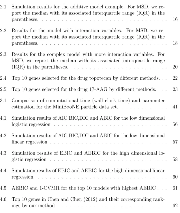
From Table 2.1, we can see that when the predictors are generated from t(4), a heavy-tailed distribution, HZ-SIS performs best, followed by MV-SIS, DC-SIS and Qa-SIS. This result, combined with the fact that HZ-SIS requires fewer assump-tions for the sure screening property, indicates that HZ-SIS is a more robust feature screening method than the existing ones. When the predictors are generated from
Table 2.1: Simulation results for the additive model example. For MSD, we report the median with its associated interquartile range (IQR) in the parentheses.
Method MSD P1 P2 P3 P4 Pa SIS 976.50(1023.00) 0.07 0.08 0.96 0.98 0.01 NIS 1342.50(704.75) 0.01 0.20 0.05 0.76 0.00 DC-SIS 279.50(656.75) 0.27 0.46 0.57 0.95 0.16 Case 1 MV-SIS 24.00(118.00) 0.83 0.73 0.97 0.95 0.58 Qa-SIS 347.50(653.50) 0.02 0.81 0.22 0.98 0.00 HZ-SIS 11.50(22.00) 0.98 0.90 0.97 0.94 0.80 SIS 1216.50(964.75) 0.10 0.02 1.00 1.00 0.00 NIS 924.00(1257.25) 0.16 0.17 0.30 0.33 0.06 DC-SIS 197.00(339.00) 0.20 0.31 0.98 0.98 0.06 Case 2 MV-SIS 11.00(28.00) 0.94 0.83 1.00 1.00 0.78 Qa-SIS 8.00(15.50) 0.91 0.91 1.00 1.00 0.82 HZ-SIS 24.50(52.25) 0.71 0.88 0.99 1.00 0.64
the uniform distribution, for which the support is bounded, HZ-SIS still performs reasonably well. In this case, it is comparable with MV-SIS and Qa-SIS, but much better than DC-SIS, NIS and SIS.
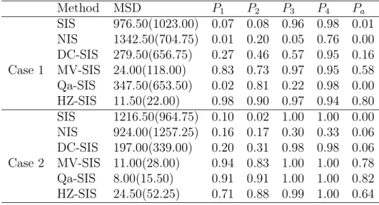
For the case where the predictors are generated from t(4) distribution, we also plotted histograms of the calculated screening indices of each method. Specifically, for each method, we first combined the corresponding screening indices from 100 simulations. Then we drew a histogram using all 400 indices from active variables and a histogram using 600 indices from inactive variables, which are randomly selected from a total of 199,600(100×1996) ones. Finally, we put two histograms in the same figure and differentiated them by color. The histograms are shown in Figure 2.1. It is clear that HZ-SIS has the smallest overlapping area for its two histograms, which again confirms its superiority in separating active features and inactive ones.
Figure 2.1: Histograms of the screening indices of different methods for the additive model example with the predictors generated from the distribution t(4).
2.3.2 A Model with Interaction Variables
This example illustrates the performance of HZ-SIS for the models with interac-tion variables. Let
Y = 0.5 + 10X1 1 +X2
50 +ε,
The vector of covariates X = (X1,· · · , Xp)T is generated from the multivariate normal distribution having mean 0 and the covariance matrix Σ = (σij)p×p with
σij = 0.5|i−j|. For the error term ε, we considered two cases: (i) follows N(0,12) distribution. (ii)followst(1)distribution. We set(n, p) = (200,1000)and repeated each experiment for 100 times.
Jiang and Liu (2014) recently proposed a procedure, called sliced inverse regres-sion for interaction detection (SIRI), to conduct high dimenregres-sional variable selection
for the model with interaction terms. Instead of building a predictive model of the response given combinations of predictors, this procedure is based on modeling the conditional distribution of predictors given responses. Since this procedure includes a screening step, so we also implemented this step here and denoted it as SIRI-SIS.
In SIRI-SIS, we used a fixed slicing scheme with 10 slices of equal size (H=10). In Qa-SIS procedure, we set τ = 0.4 and the number of basis dn = [n
1
5] = 3. The
results are summarized in Table 2.2.
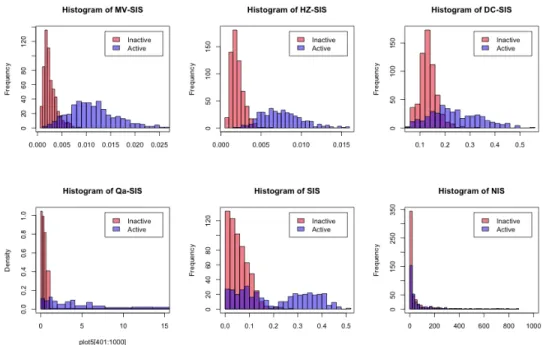
Table 2.2: Results for the model with interaction variables. For MSD, we report the median with its associated interquartile range (IQR) in the parentheses.
Method MSD P1 P50 Pa SIS 686.00(321.25) 1.00 0.00 0.00 SIRI-SIS 3.00(1.00) 1.00 0.99 0.99 DC-SIS 50.50(52.25) 1.00 0.39 0.39 Case 1 MV-SIS 34.00(73.75) 1.00 0.52 0.52 Qa-SIS 426.00(478.00) 1.00 0.02 0.02 HZ-SIS 3.00(1.00) 1.00 1.00 1.00 SIS 575.50(387.00) 0.78 0.03 0.01 SIRI-SIS 11.00(52.00) 1.00 0.69 0.69 DC-SIS 167.00(251.25) 1.00 0.12 0.12 Case 2 MV-SIS 97.50(158.75) 1.00 0.23 0.23 Qa-SIS 414.50(403.75) 1.00 0.02 0.02 HZ-SIS 9.50(22.00) 1.00 0.86 0.86
Table 2.2indicates that in the case where error term is normal, all methods can detect X1 with ease, but when it comes to detecting X50, HZ-SIS and SIRI-SIS substantially outperforms other methods. For the case where error term follows t(1) distribution, we have similar conclusions as in the normal case. In addition, our method performs slightly better than SIRI-SIS in this case.
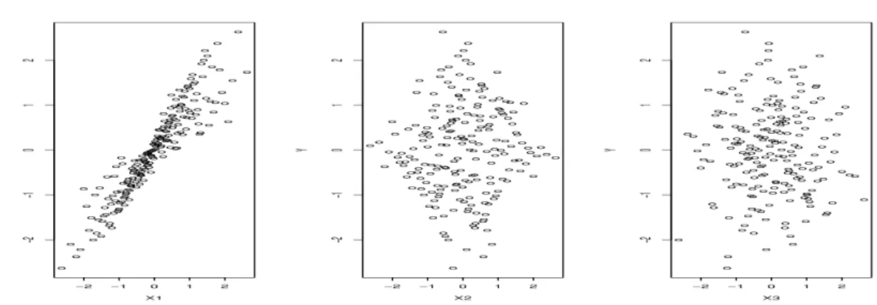
scat-ter plots of the transformed predictors Te1(X1), Te50(X50) and Te100(X100) versus the transformed response variableTey(Y)in case 1. The scatter plots ofX1,X50andX100 versusY are similar. Given the reference scatter plot of(Te100(X100),Tey(Y))for which
the theoretical joint distribution is N(0, I2), we can see that the joint distributions of (Te1(X1),Tey(Y)) and (Te50(X50),Tey(Y)) substantially deviate from N(0, I2), and
thereby HZ-test is powerful in detecting the dependence of Y on X1 and X50. How-ever, not all other methods work well for this example. As indicated by the values of P2 reported in Table 2.2, SIS and Qa-SIS essentially fail to detect the dependence of Y on X50, and DC-SIS and MV-SIS have only limited success probabilities of detecting this dependence.
Figure 2.2: Scatter plots of the transformed response variable Tey(Y) versus the
transformed predictors Te1(X1), Te50(X50) and Te100(X100)
2.3.3 A Complex Model with More Interaction Variables
This example illustrates the performance of HZ-SIS for more complex models. Let
Y = 1 +A[10X1+ exp(X22+ 3X3)] + 10
X5 2 +X6
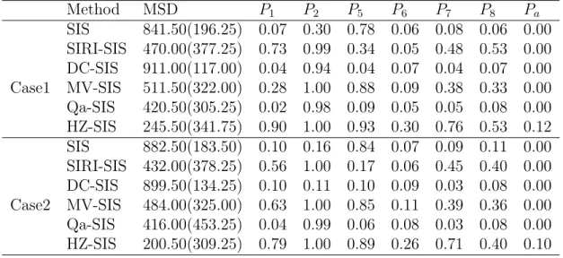
Table 2.3: Results for the complex model with more interaction variables. For MSD, we report the median with its associated interquartile range (IQR) in the parentheses.
Method MSD P1 P2 P5 P6 P7 P8 Pa SIS 841.50(196.25) 0.07 0.30 0.78 0.06 0.08 0.06 0.00 SIRI-SIS 470.00(377.25) 0.73 0.99 0.34 0.05 0.48 0.53 0.00 DC-SIS 911.00(117.00) 0.04 0.94 0.04 0.07 0.04 0.07 0.00 Case1 MV-SIS 511.50(322.00) 0.28 1.00 0.88 0.09 0.38 0.33 0.00 Qa-SIS 420.50(305.25) 0.02 0.98 0.09 0.05 0.05 0.08 0.00 HZ-SIS 245.50(341.75) 0.90 1.00 0.93 0.30 0.76 0.53 0.12 SIS 882.50(183.50) 0.10 0.16 0.84 0.07 0.09 0.11 0.00 SIRI-SIS 432.00(378.25) 0.56 1.00 0.17 0.06 0.45 0.40 0.00 DC-SIS 899.50(134.25) 0.10 0.11 0.10 0.09 0.03 0.08 0.00 Case2 MV-SIS 484.00(325.00) 0.63 1.00 0.85 0.11 0.39 0.36 0.00 Qa-SIS 416.00(453.25) 0.04 0.99 0.06 0.08 0.03 0.08 0.00 HZ-SIS 200.50(309.25) 0.79 1.00 0.89 0.26 0.71 0.40 0.10
where A is generated from the set {−1,1} with equal probability, Xk’s are indepen-dently generated from t(4) distribution. For the error term ε, we considered two cases: (i) follows N(0,12) distribution. (ii) followst(1) distribution. This model is complex, containing more interaction variables than previous examples. We set (n, p) = (400,1000)and repeated each experiment 100 times.
In SIRI-SIS, we used a fixed slicing scheme with 10 slices of equal size (H=10). In Qa-SIS procedure, we set τ = 0.4 and the number of basis dn = [n
1
5] = 3. The
results are summarized in Table 2.3.
From Table 2.3, we can see that in both case, HZ-SIS has an overall superior performance against the other methods.
2.4 Screening of Anticancer Drug Response Genes
Recent advances in high-throughput biotechnologies, such as microarray, sequenc-ing technologies and mass spectrometry, have provided an unprecedented opportunity for biomarker discovery. Molecular biomarkers can not only facilitate disease
diagno-sis, but also reveal underlying, biologically distinct, patient subgroups with different sensitivities to a specific therapy. The latter is known as disease heterogeneity, which is often observed in complex diseases such as cancer. For example, molecularly tar-geted cancer drugs are only effective for patients with tumors expressing targets (Grünwald and Hidalgo, 2003; Buzdar, 2009). The disease heterogeneity has directly motivated the development of precision medicine, which aims to improve patient care by tailoring optimal therapies to an individual patient according to his/her molecular profile and other clinical characteristics.
Toward the ultimate goal of precision medicine, i.e., selecting right drugs for individual patients, a recent large-scale pharmacogenomics study, namely, cancer cell line encyclopedia (CCLE), has screened multiple anticancer drugs over hundreds of cell lines in order to elucidate the response mechanism of anticancer drugs. The dataset consists of the dose-response data for 24 chemical compounds across over 479 cell lines. For each cell line, it consists of the expression data of 18,988 genes. The dataset is publicly available atwww.broadinstitute.org/ccle. Our goal is to screen the genes that respond to each chemical compounds, which will facilitate the followed analysis for identification of anticancer drug response genes. In our analysis, we used the area under the dose-response curve, which is termed as activity area in Barretina
et al. (2012), to measure the sensitivity of drug to a given cell line. Compared to other measurements, such as IC50 and EC50, the activity area could capture the efficacy and potency of a drug simultaneously.
The drug topotecan (trade name Hycamtin) is a chemotherapeutic agent that is a topoisomerase inhibitor. It is a synthetic, water-soluble analog of the natural chemical compound camptothecin and has been used to treat ovarian cancer, lung cancer and other cancer types. After GlaxoSmithKline received final FDA approval for Hycamtin Capsules in 2007, topotecan became the first topoisomerase I inhibitor
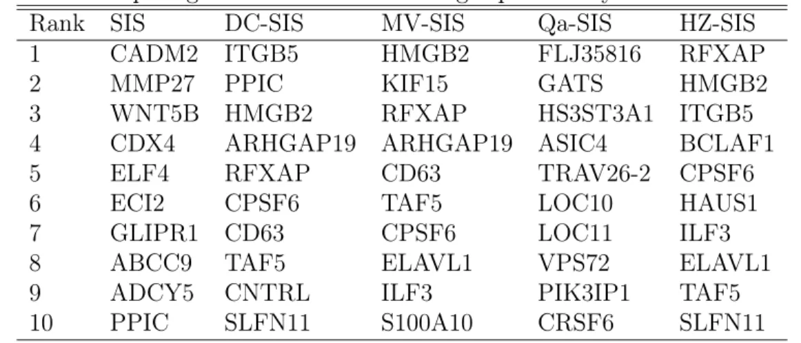
Table 2.4: Top 10 genes selected for the drug topotecan by different methods.
Rank SIS DC-SIS MV-SIS Qa-SIS HZ-SIS
1 CADM2 ITGB5 HMGB2 FLJ35816 RFXAP
2 MMP27 PPIC KIF15 GATS HMGB2
3 WNT5B HMGB2 RFXAP HS3ST3A1 ITGB5
4 CDX4 ARHGAP19 ARHGAP19 ASIC4 BCLAF1
5 ELF4 RFXAP CD63 TRAV26-2 CPSF6
6 ECI2 CPSF6 TAF5 LOC10 HAUS1
7 GLIPR1 CD63 CPSF6 LOC11 ILF3
8 ABCC9 TAF5 ELAVL1 VPS72 ELAVL1
9 ADCY5 CNTRL ILF3 PIK3IP1 TAF5
10 PPIC SLFN11 S100A10 CRSF6 SLFN11
for oral use. Table 2.4 lists the top 10 important genes selected for topotecan by HZ-SIS. For comparison, the table also includes the top 10 genes selected by SIS, DC-SIS, MV-SIS and Qa-SIS. In Qa-SIS procedure, we setτ = 0.5and the number of basis dn = [n
1
5] = 3. For topotecan, the gene SLFN11 has been recognized as a very
important predictor for the sensitivity of topotecan (Barretina et al., 2012; Zoppoli
et al., 2012). HZ-SIS ranks it No. 10. In addition to SLFN11, Wang et al. (2014) found the strong relevance of HMGB2 and BCLAF1 to topotecan. HZ-SIS ranks these two genes No. 2 and No. 4, respectively. DC-SIS has a similar performance to HZ-SIS for the drug topotecan, while the other methods do not.
The drug 17-AAG is a derivative of the antibiotic geldanamycin that is being studied in the treatment of cancer, specific young patients with certain types of leukemia or solid tumors, especially kidney tumors. 17-AAG works by inhibiting the gene HSP90, which is expressed in those tumors, and belongs to the family of drugs called antitumor antibiotics. Table 2.5 reports the top 10 genes ranked by different methods for 17-AAG. According to Hadley and Hendricks (2014) and Barretinaet al.
Table 2.5: Top 10 genes selected for the drug 17-AAG by different methods.
Rank SIS DC-SIS MV-SIS Qa-SIS HZ-SIS
1 UXT NQO1 NQO1 MMP24 NQO1
2 IGFN1 MMP24 INO80 ATP6V0E1 OGDHL
3 MSH2 ZNF610 MMP24 ZFP30 TMEM198
4 ROCK1 ZFP30 ZNF610 GPR35 ZBTB7A
5 DDA1 NFKB1 ZFP30 SLC1A5 GYG2
6 SCEL CDH6 PRPUSD4 GPX2 CDH6
7 ST5 OGDHL LOC10 CNTRL ZNF610
8 THUMPD3 LOC10 PCSK1N VPS72 RPUSD4
9 ITGA9 PRUSD4 NFKB1 LOC10 CSK
10 C20orf141 IN080 ZBTB7A ZNF610 CTCF
3. DOUBLE-PARALLEL MONTE CARLO FOR BAYESIAN ANALYSIS OF BIG DATA
3.1 Introduction
The MCMC method has proven to be a very powerful and typically unique com-putational tool for analyzing data of complex structures. However, it is difficult to be applied to big data problems for which complex models are often needed. The difficulty comes from two aspects. The first one is on data storage; the dataset can be too large for a single computer to store and process. The second one is on computational time; the MCMC method can be very time consuming for simulating from the posterior of a large data set, which typically requires a large number of iterations and a complete scan of the full dataset for each iteration. However, thanks to strategy of embarrassingly parallel computing, the two issues can now be solved simultaneously.
The strategy of embarrassingly parallel computing is to divide a large dataset into a number of smaller subsets such that each subset can be stored in a single machine, and then conduct the Bayesian analysis for each subset separately. Finally, the posterior samples generated for each subset are aggregated in some way such that a correct inference can be made for the full data posterior. During the past few years, this strategy has been pursued by a few groups enthusiastically. Several algorithms have been developed to address the issue of subset posterior aggregation. To be a little more detailed, suppose that a large dataset has been partitioned into k subsets, and N posterior samples have been generated for each subset. Let {θ(i)1 , . . .θ(i)N} denote the posterior samples generated from subset i. Based on the Bernstein-von Mises theorem, which states that the posterior tends to a normal
distribution centered around the true parameter value θ∗ as the number of obser-vations grows, Scott et al. (2016) proposed to use the weighted average Pk
i=1wiθ (i) j to approximate a full data posterior sample, where the weight wi is the inverse of the covariance matrix of {θ(i)1 , . . .θ(i)N}. This algorithm is exact when the subset posterior is exactly Gaussian. Based on the same theory, Neiswanger et al. (2013) proposed to fit the posterior samples generated for each subset by a Gaussian den-sity, denoted the fitted density by pˆi for i = 1, . . . , k, and then draw samples from the product density pˆ1. . .pˆk. As an extension of this approach, Neiswanger et al. (2013) also proposed to estimate the subset posterior density using a Gaussian kernel density estimation method or a semiparametric density estimation method. Wang and Dunson (2013) proposed a Weierstrass refinement sampler, where the samples from an initial approximation to the full data posterior (e.g., obtained via variational approximation or other methods) are refined using the information obtained from the subset posterior samples within a Weierstrass approximation. Another method that makes use of kernel approximation is by Minsker et al.(2014), where the subset pos-teriors are combined by estimating a probability distribution that minimizes a loss function defined in the reproducing kernel Hilbert space embedding the subset pos-teriors. These methods generally work well, but their accuracy can vary significantly depending on how close the subset posteriors are to Gaussian or the choice of kernel and its bandwidth. In particular, their accuracy can be low when the dimension of θ is high. Quite recently, the so-called WASP method was proposed by Srivastava
et al. (2015), where each subset posterior is approximated by an empirical measure and they are combined by estimating their barycenter in the Wasserstein space of probability measures. This method does not depend on the kernel density estimation any more, but computing the Wasserstein barycenter needs to solve a huge linear programming problem which often requires a lot of computer memory.
In this chapter, we introduce a new method for aggregating subset posterior samples. The new method is surprisingly simple, which is to first simulate from some modified subset posteriors, for which the log-likelihood functions are appropriately scaled according to their sample size, and then recenter the subset posterior samples to their global mean. Under mild conditions, we show that the aggregated samples have the same convergence rate toward the true parameter θ∗ as those drawn from the full data posterior. The numerical results indicate that the new method can be rather accurate compared to the existing ones. In order to further speed up computation, we suggest to use the Pop-SAMC algorithm (Songet al., 2014), rather than traditional single chain MCMC algorithms, to draw samples from each subset posterior. Since the proposed method consists of two levels of parallel, data parallel and simulation parallel, it is coined as “double parallel” Monte Carlo.
The remainder of this chapter is organized as follows. Section 3.2 presents the proposed sample aggregation method and describes its theoretical properties. Section 3.3 first gives a brief review of the pop-SAMC algorithm, and then discusses the double parallel strategy. Sections 3.4 and 3.5 present some numerical results along with some comparisons with the existing methods.
3.2 Subset Posterior Aggregation
Suppose that a random sample X = {X1, . . . , Xn} has been collected from the distribution f(x|θ∗), where θ∗ ∈ Θ ⊂ Rp and Θ is the parameter space. Let g(θ) denote the prior distribution of θ. Then the posterior distribution of θ is given by
π(θ|X) = Qn i=1f(Xi|θ)g(θ) R Θ Qn i=1f(Xi|θ)g(θ)dθ . (3.1)
In most cases,π(θ|X)is analytically intractable and we have to approximate it using the Markov chain Monte Carlo(MCMC) method. However, as mentioned previously,
when n is very large, the MCMC method is computationally prohibitive because it requires a large number of scans of the dataset.
To address this issue, we divide the data into k subsets, each containing about the same number of samples. Let X[j] = (Xj1, . . . , Xjmj) denote the jth subset, where
mj denote the sample size of X[j]. Let π(θ|X[j]) denote the posterior distribution corresponding to the subsetX[j], for which the variance is approximatelyn/mj times the variance of full data posterior π(θ|X). To adjust the variance, for each subset, we instead work on a modified subset posterior
˜ π(θ|X[j]) = Qm i=1f n/mj(X ji|θ)π(θ) R Θ Qm i=1fn/mj(Xji|θ)π(θ)dθ , (3.2)
where each sample is duplicated n/mj times. Such a modification, first introduced in Minsker et al. (2014), ensures that π˜(θ|X[j]) has about the same variance as the full data posterior. In what follows, we refers to π˜(θ|X[j]) as a subposterior and, without loss of generality, assume that m1 =m2 =· · ·=mk =m holds.
Letµ(1),· · · ,µ(k) denote the mean of the subposteriors, and letµˆ = 1 k
Pk
j=1µ(j) denote their averages. We propose to recenter each of the subposteriors to µˆ and then use the following mixture of re-centered subposteriors to approximate the full data posterior π(θ|X): ˜ π(θ|X) = 1 k k X j=1 ˜ π(θ+ ( ˆµ−µ(j))|X[j]). (3.3) To quantify the accuracy of the approximation, we make the following assump-tions:
(A1) The log-likelihood function Pm
i=1logf(xji|θ) is Laplace-regular for each j = 1, . . . , k.
(A2) θ∗ is an interior point of Θ, g(θ∗) > 0, and g(θ) is four times continuous differentiable on Θ.
(A3) The number of subsetskcan increase slowly withn, but can not exceedO(n1/2). Since the quantification involves posterior expansions based on Laplace’s method, the Laplace regularity condition is assumed. Refer to Kass et al. (1990) for the detail. This condition is standard and generally holds for the exponentially family. Under the above conditions, we have the following theorem, whose proof is given in the appendix.
Theorem 3.1. If the conditions (A1)-(A3) are satisfied, then we have
E[Eπ˜(θ)−Eπ(θ)]2 = O(m−2), (3.4) E|Varπ˜(θ)−Varπ(θ)| = o(n−1), (3.5) E(d2(π, δθ∗)) = 2 tr(I−1) n +o(n −1), (3.6) E(d2(˜π, δθ∗)) = 2 tr(I−1) n +o(n −1), (3.7)
where Eπ and E˜π denote the expectations with respect to π and π˜, respectively;
Varπ and Varπ˜ denote the variances with respect to π and π˜, respectively; I = −EX|θ∗∂
2logf(X|θ(∗))
∂θ∂θT is the Fisher information matrix, and d
2(˜π, δ
θ∗) = R
Θkθ − θ∗k2
2π˜(θ|X)dθ is the Wasserstein distance of order 2 between π˜(θ|X)and the Dirac
measure at θ∗.
Equations (3.4) and (3.5) measure the accuracy of the approximationπ˜(θ|X)to
π(θ|X) in terms of mean and variance, respectively. In particular, equation (3.4) implies that π˜(θ|X) and π(θ|X) will lead to the same Bayesian estimate (with respect to the square loss function), and equation (3.5) implies that the Bayesian
estimates led from π˜(θ|X) and π(θ|X) will have about the same variance when
n is large. Equations (3.6) and (3.7) imply that π˜(θ|X) and π(θ|X) share the same convergence rate toward the true value θ∗. In other words, the subposterior aggregation does not lose much information about the data.
Rather thanθ itself, sometimes we are interested in h(θ), a Rp 7→Rq function of θ. A similar result, which measures the accuracy of the approximation π˜(h(θ)|X), can be obtained under the following condition:
(A4) h(θ)is square integrable and thrice times continuous differentiable in a neigh-borhood of θ∗.
Corollary 3.1. If A1-A4 are satisfied, then we have
E[E˜πh(θ)−Eπh(θ)]2 = O(m−2), E|V arπ˜h(θ)−V arπh(θ)| = o(n−1), E(d2(π(h(θ)|X), δh(θ∗))) = 2 tr(H(1)∗ I−1H∗0 (1)) n +o(n −1), E(d2(˜π(h(θ)|X), δh(θ∗))) = 2 tr(H(1)∗ I−1H∗0 (1)) n +o(n −1 ), whereH(1)∗ = ∂h(θ)
∂θT |θ=θ∗, and Iis the Fisher information matrix as defined in Theorem
3.1.
The proof is similar to that of Theorem 3.1, which is based on the expansion for the posterior mean of h(θ)and thus omitted here.
3.3 Double Parallel Monte Carlo
In this section, we first give a brief review of the Pop-SAMC algorithm and discuss its implementation on the OpenMP platform. Then we describe the double parallel Monte Carlo scheme.
3.3.1 Pop-SAMC Algorithm and Its OpenMP Implementation
As aforementioned, although MCMC is powerful for analyzing the data of com-plex structures, its computer-intensive nature precludes its use for big data analysis. To accelerate computation, one feasible way is to conduct parallel MCMC simula-tions. People have debated for a long time to make a single long run or many short runs. For conventional MCMC algorithms, such as the Metropolis-Hastings algo-rithm(Metropolis et al., 1953; Hasting, 1970) and the Gibbs sampler (Geman and Geman, 1984), parallel runs may not provide any theoretical advantages over a single long run. In general, if you cannot get a good answer with a long run, then you can-not get a good answer with many short runs either. However, this situation differs for the population stochastic approximation Monte Carlo (pop-SAMC) algorithm (Song
et al., 2014), where it is shown that running pop-SAMC with κ chains (in parallel) for T iterations is asymptotically more efficient than running a single SAMC chain for κT iterations when the gain factor sequence decreases slower thanO(1/t), where
t indexes iterations. This is due to that the chains in pop-SAMC interact with each other intrinsically.
The pop-SAMC algorithm consists of two steps, population sampling and ξ-updating, where ξ denotes an adaptive parameter evolving with iterations. In the population sampling step, each chain is updated independently for one or a few iterations. In the ξ-updating step, ξt (i.e., the value of ξ at iteration t) is updated based on the collected information from individual chains, which enforces interactions between different chains and, consequently, improves the efficiency of the algorithm. The detailed algorithm is described below.
Suppose that we are interested in simulating samples from a density function
u1}, E2 = {θ : u1 ≤ U(θ) < u2}, . . ., EM−1 = {θ : uM−2 ≤ U(θ) < uM−1}, and EM = {θ : U(θ) ≥ uM−1}, where U(θ) is a pre-specified function of θ, e.g.,
U(θ) = −logp(θ), and u1 < u2 < · · · < uM−1 are pre-specified numbers. To explain the concept of SAMC, we assume for the time being that all the subregions are non-empty; that is, zi =
R
Eip(θ)dθ > 0 for all i = 1, . . . , M. However, as
explained in Liang et al. (2007), the algorithm does allow the existence of empty subregions. Let π = (π1, . . . , πM)denote the desired sampling distribution of the M subregions, where PM
i=1πi = 1 and πi >0 for all i = 1, . . . , M. Given the partition and the desired sampling distribution, Pop-SAMC seeks to draw samples from the distribution pz(θ)∝ M X i=1 πip(θ) zi I(θ ∈Ei).
If zi’s are known and the space is partitioned appropriately, e.g., the energy band-width of each subregion is small enough, then the sampling will lead to a random walk in the space of subregions and thus the local-trap problem can be overcome essentially. However, since z1, . . . , zM are generally unknown, Pop-SAMC employs the stochastic approximation algorithm (Robbins and Monro, 1951) to learn their values (up to a constant factor) in an adaptive way.
Let κ denote the population size, i.e., the number of parallel Markov chains contained in Pop-SAMC, and let θt = (θt1, . . . ,θtκ) denote the current state of the
κ chains. Letξt= (ξt1, . . . , ξtM) denote the working estimate of(z1/π1, . . . , zM/πM) obtained at iterationt. One iteration of the algorithm consists of the following steps: 1. (Population sampling) For i = 1, . . . , κ, generate a new sample θt,i starting
from θt−1,i by a single MH update with the target distribution given by
pξt−1(θ)∝ M X j=1 p(θ) eξt−1,jI(θ∈Ej). (3.8)
2. (ξ-update) Set ξt = ξt−1 +γt(Ht − (1/M)1), where Ht = (Pκi=1I(θt,i ∈
E1)/κ,· · · ,PNi=1I(θt,i ∈EM)/κ)T, and γt is a gain factor.
To ensure the convergence of the algorithm, the gain factor {γt} is required to satisfy the conditions:
∞ X t=1 γt=∞, γt+1−γt γt =O(γt+1τ ), ∞ X t=1 γt(1+τ0)/2 √ t <∞,
for some τ ∈ [1,2) and τ0 ∈ (0,1). For example, one can set γt = O(1/tζ) for
ζ ∈ (1/2,1]. To accommodate the case that ξt takes values in an unbounded space, a varying truncation version of the algorithm can be considered as in Andrieu et al.
(2005).
Like the SAMC algorithm(Liang et al., 2007), Pop-SAMC possesses the self-adjusting mechanism, which operates based on past samples and enables the simula-tion to be immune to local traps. This can be considered as a significant advantage over conventional MCMC algorithms, such as the Metropolis-Hastings algorithm and the Gibbs sampler. Also, we would like to state that the pop-SAMC algorithm is essentially a dynamic importance sampling algorithm for which the trial distribu-tion, i.e., the working target distribution (3.8), changes from iteration to iteradistribu-tion, and the quantities of interest can be estimated through weighted averaging as in conventional importance sampling (Liang, 2009). That is, Pop-SAMC generates a sequence of importance samples {(θt,1, e
ξt,J(θt,1)), . . . ,(θ
t,κ, eξt,J(θt,κ))}, where J(θt,i) denotes the index of the subregion that θt,i belongs to, and e
ξt,J(θt,i) specifies the
importance weight of θt,i.
OpenMP is an application programming interface (API) for parallel programming on multi-core CPUs which are now available in regular desktops/laptops. It works in a shared memory mode with the fork/join parallelism, and is particularly suitable
for pop-SAMC. To be precise, the population sampling step of pop-SAMC can be carried out in parallel through the pragmaomp parallelto fork multiple threads with each thread running for an individual Markov chain. After the parallel execution, the threads join back to the master thread, whereξtis updated based on the information collected from the multiple threads. Since OpenMP works in a shared memory mode, distributing the updated ξt to different threads is avoided. Since the population sampling steps cost the major portion of the CPU, the parallel execution provides a nearly linear speedup for the simulation.
3.3.2 Double Parallel Monte Carlo
Based on the subposterior aggregation theory studied in Section 2 and the Pop-SAMC algorithm, we suggest the following double parallel Monte Carlo algorithm for Bayesian analysis of big data.
• (Data Parallel) Divide the dataset into k subsets with each containing about the same sample size.
• (Simulation Parallel) Run Pop-SAMC for each subposterior π˜(θ|X[i]) sepa-rately. Let {(θ(i)1 , w(i)1 ), . . ., (θ(i)N, w(i)N)} denote the importance samples gener-ated by Pop-SAMC from π˜(θ|X[i]) for i = 1, . . . , k. Let µˆ(i) =
PN j=1w (i) j θ (i) j PN j=1w (i) j
denote the mean of the subposterior π˜(θ|x[i]).
• (Sample aggregation) Calculate the global meanµˆ =Pk
i=1µˆ
(i)/k, recenter the importance samples as {(θ(i)1 −µˆ(i) + ˆµ, w(i)1 ), . . . ,(θ(i)N −µˆ(i) + ˆµ, w(i)N)} for
i= 1, . . . , k.
Then, for each i= 1,2, . . . , k, the re-centered samples can be viewed as a batch of importance samples generated from the full data posterior. For any function
b ρ1 = Pk i=1ρb (i) 1 /k, where ρb (i) 1 = PN j=1w (i) j h(θ (i) j −µˆ (i) + ˆµ)/PN j=1w (i) j . Alternatively, ρ can be estimated by b ρ2 = Pk i=1 PN j=1w (i) j h(θ (i) j −µˆ (i)+ ˆµ) Pk i=1 PN j=1w (i) j . Let Ui = PN j=1w (i) j h(θ (i) j −µˆ (i) + ˆµ), Si = PN j=1w (i) j ,S =E(Si), andVi =Ui−ρSi. Following from the property of SAMC, the variances of Ui and Vi are both finite. Then the standard error of ρb2 can be calculated as for the ratio estimate (Ripley, 1987). The Vi’s can be treated as iid random variables with zero mean and finite variance, and its variance can be estimated by σˆ2
V = 1/k
Pk
i=1V 2
i . The law of large numbers implies that 1/√kPk
i=1Vi is asymptotically normal N(0, σ 2 V) and that √ k(ρb2−ρ) = 1 √ k Pk i=1Vi 1 k Pk i=1Si →N(0, σ2), where σ2 =σ2
V/S2, and it can be estimated by σˆ2V/Sˆ2 with Sˆ=
Pk
i=1Si/k. 3.4 Simulation Study
3.4.1 Logistic Regression
The first example is very simple, whose goal is to show the validity of the pro-posed subposterior aggregation method. The example is adopted from Srivastava
et al. (2015). It is for a logistic regression with n = 104 and the true parameter θ∗ = (1,−1)T. The covariatesZ
1 andZ2 are drawn from the standard Gaussian dis-tribution. The prior distribution of θ is N(0, I2). To follow the notation in Section 3.2, we let X = (Y, Z1, Z2).
To implement the proposed double parallel algorithm, we randomly divided the dataset into 10 subsets with each consisting of 1000 samples. Then Pop-SAMC was
run for each subset. Specifically, for each subset, we partitioned the parameter space Θ according to the energy function U(θ) = −logpj(θ) with an equal bandwidth ∆u= 0.5into five subregionsE1 ={θ:U(θ)< u+ 0.5},E2 ={θ :u+ 0.5≤U(θ)<
u+ 1}, E3 ={θ :u+ 1 ≤U(θ)< u+ 1.5} E4 ={θ :u+ 1.5≤U(θ)< u+ 2}, and
E5 ={θ :U(θ)≥u+ 2}, wherepj denote the subposterior of the jth subset, and u was chosen as the smallest value of U(θ) obtained in a preliminary trial. The gain factor γt was set as 100/max(100, t). The proposal was set as a Gaussian random walk distribution with the covariance matrix 0.22I2. The population size was set to
N = 10and the number of iterations was set toT = 105. The first104iterations were discarded for the burn-in process, and samples were collected from the remainder of the run at every 5 iterations. In total, we had1.8×105 importance samples collected at the end of each run.
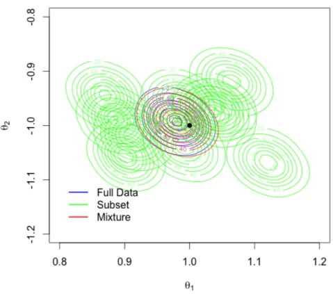
Figure 3.1 shows the contour plots of the full data posterior π(θ|X), each sub-posterior π˜(θ|X[j]), and the proposed mixture posterior π˜(θ|X). The R package KernSmooth was used to generate the corresponding binned kernel density esti-mates. The plots indicate that each subposterior has a similar shape with the full data posterior, however, most of them have a notably biased center from the true parameter θ∗. By shifting the mean of each subposterior to the global mean, the bias was successfully removed. The mixture posterior π˜(θ|X) closely matches the full data posterior π(θ|X).
3.4.2 Linear Regression with Unknown Variance
We use this example to compare the accuracy of the approximations to the full data posterior by the proposed algorithm, WASP(Srivastava et al., 2015) and con-sensus Monte Carlo(Scott et al., 2016). The example was adopted from Liang et al.
Figure 3.1: Binned kernel posterior density estimates for the parameters of a logistic regression. The true parameter θ∗ = (1,−1)T (black dot).
(2016), which is about a normal linear regression with unknown variance:
yi =β0+β1zi1+β2zi2+β3zi3+i, i= 1,2, . . . , n
where (β0, β1, β2, β3) = (2,0.25,0.25,0) the true regression coefficients, in addition,
1,· · · , n are i.i.d. normal random errors with mean 0 and variance σ2 = 0.25. The covariates z1 and z2 are drawn from standard normal distributions independently. The covariatez3 = 0.7z2+0.3e, whereealso follows the standard normal distribution. Under this setting, z2 and z3 are highly correlated with a correlation coefficient of
0.919. We generated n = 104 samples from this model. For this example, we are to estimate both the regression coefficients and the variance of the random error, i.e., θ = (β0, β1, β2, β3, σ2). For the regression coefficients, we use non-informative prior
g(β0, β1, β2, β3)∝1; for the varianceσ2, we use the priorg(σ2)∝(1σ)1/1000. To follow the notation in Section 3.2, we set Xi = (yi, zi1, zi2, zi3).
For the double parallel algorithm, we randomly divided the dataset into 10 subsets with each consisting of 1000 samples. Pop-SAMC was run for each subset separately with the same setting as for the previous example except that the energy bandwidth was set to ∆u= 2 and the covariance matrix of the Gaussian random walk proposal distribution was set to 0.012I
5. For comparison, consensus Monte Carlo and WASP were also applied to this example. For WASP, due to the limitation of memory, we only used 300 posterior samples that were randomly selected from the pool of Metropolis-Hastings samples collected previously. Note that for consensus Monte Carlo, the subset posterior is defined as
Qm i=1f(Xji|θ)g1/k(θ) R Θ Qm i=1f(Xji|θ)g1/k(θ)dθ , (3.9)
which is slightly different from the subposterior defined in (3.2), the one used in WASP and double parallel.
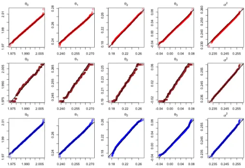
Figure 3.2 shows the QQ-plots for each of the five parameters of the model and for each of the methods, double parallel, consensus Monte Carlo and WASP, ver-sus the full data posterior simulation. The QQ plots indicate that double parallel and consensus Monte Carlo can provide more accurate approximations to the full data posterior than WASP. Regarding efficiency of the three algorithms, we com-pared the rough number of effective samples produced by them with the same CPU time. Within a given CPU time, the double parallel algorithm produced 1.8×10⁶
Figure 3.2: QQ-plots for the normal regression example. The top, middle and bottom panels are for the double parallel, WASP and consensus Monte Carlo, respectively.
importance samples (1.8× 10⁵ importance samples were collected for each of the 10 subsets). However, consensus Monte Carlo produced only 1.8×10⁵ samples, for which the samples produced by different chains (each for a different subset) are av-eraged to get the final samples. For WASP, the samples produced by different chains do not need to be averaged, but need to be weighted through linear programming in estimating their Wasserstein barycenter. Again, the importance weighting procedure will significantly reduce its effective sample size.
3.5 A Big Data Example
The goal of this example is to show how efficient the double parallel algorithm can be compared to the traditional single chain MCMC algorithm for a big data problem. For this purpose, we applied the double parallel algorithm to the MiniBooNE particle identification dataset, which is available at the UCI machine learning repository.
![中文文字蘊涵系統之特徵分析 (Feature Analysis of Chinese Textual Entailment System) [In Chinese]](data:image/gif;base64,R0lGODlhAQABAIAAAP///wAAACH5BAEAAAAALAAAAAABAAEAAAICRAEAOw==)