Combining Representation Learning with Logic for Language Processing

(1)

Combining Representation Learning

with Logic for Language Processing

Tim Rockt¨aschel

A dissertation submitted in partial fulfillment of the requirements for the degree of

Doctor of Philosophy of

University College London.

Department of Computer Science University College London

(2)

(3)

(4)

(5)

Acknowledgements

I am deeply grateful to my supervisor and mentor Sebastian Riedel. He always has been a great source of inspiration and supportive and encouraging in all matters. I am particularly amazed by the trust he put into me from the first time we met, the freedom he gave me to pursue ambitious ideas, his contagious optimistic attitude, and the many opportunities he presented to me. There is absolutely no way I could have wished for a better supervisor.

I would like to thank my second supervisors Thore Graepel and Daniel Tarlow for their feedback, as well as Sameer Singh whose collaboration and guidance made my start into the Ph.D. very smooth, motivating, and fun. Furthermore, I thank Edward Grefenstette, Karl Moritz Hermann, Thomas Kocisk´y and Phil Blunsom, who I was fortunate to work with during my internship at DeepMind in Summer 2015. I am thankful for the guidance by Thomas Demeester, Andreas Vlachos, Pasquale Minervini, Pontus Stenetorp, Isabelle Augenstein, and Jason Naradowsky during their time at the University College London Machine Reading lab. In addition, thanks to Dirk Weissenborn for many fruitful discussions. I would also like to thank Ulf Leser, Philippe Thomas, and Roman Klinger for preparing me well for the Ph.D. during my studies at Humboldt-Universit¨at zu Berlin.

I had the pleasure to work with brilliant students at University College London. Thanks to Michal Daniluk, Luke Hewitt, Ben Eisner, Vladyslav Kolesnyk, Avishkar Bhoopchand, and Nayen Pankhania for their hard work and trust. Ph.D. life would not have been much fun without my lab mates Matko Bosnjak, George Spithourakis, Johannes Welbl, Marzieh Saeidi, and Ivan Sanchez. Thanks to Matko, Dirk, Pasquale, Thomas, Johannes, and Sebastian for feedback on this thesis. Furthermore, I thank my examiners Luke Dickens and Charles Sutton for their extremely helpful in-depth comments and corrections of this thesis. Thank you, Federation Coffee in Brixton, for making the best coffee in the world.

Many thanks to Microsoft Research for supporting my work through its Ph.D. Scholarship Programme, and to Google Research for a Ph.D. Fellowship in Natural

(6)

Language Processing. Thanks to their generous support, as well as the funding from the University College London Computer Science Department, I was able to travel to all conferences that I wanted to attend.

I am greatly indebted and thankful to my parents Sabine and Lutz. They sparked my interest in science, but more importantly, they ensured that I had a fantastic childhood. I always felt loved, supported, and well protected from the many troubles in life. Furthermore, I would like to thank Christa, Ulrike, Tillmann, Hella, Hans, Gretel, and Walter for their unconditional support over the last years.

Lastly, thanks to the two wonderful women in my life, Paula and Emily. Thank you, Paula, for keeping up with my ups and downs during the Ph.D., your love, motivation, and support. Thank you for giving me a family, and for making us feel at home wherever we are. Emily, you are the greatest wonder and joy in my life.

(7)

Declaration

I, Tim Rockt¨aschel confirm that the work presented in this thesis is my own. Where information has been derived from other sources, I confirm that this has been indi-cated in the thesis.

(8)

(9)

Abstract

The current state-of-the-art in many natural language processing and automated knowledge base completion tasks is held by representation learning methods which learn distributed vector representations of symbols via gradient based optimization. They require little or no hand-crafted features, thus avoiding the need for most prepro-cessing steps and task-specific assumptions. However, in many cases representation learning requires a large amount of annotated training data to generalize well to unseen data. Such labeled training data is provided by human annotators who often use formal logic as the language for specifying annotations.

This thesis investigates different combinations of representation learning meth-ods with logic for reducing the need for annotated training data, and for improving generalization. We introduce a mapping of function-free first-order logic rules to loss functions that we combine with neural link prediction models. Using this method, logical prior knowledge is directly embedded in vector representations of predicates and constants. We find that this method learns accurate predicate representations for which no or little training data is available, while at the same time generalizing to other predicates not explicitly stated in rules. However, this method relies on grounding first-order logic rules, which does not scale to large rule sets. To overcome this limitation, we propose a scalable method for embedding implications in a vector space by only regularizing predicate representations. Subsequently, we explore a tighter integration of representation learning and logical deduction. We introduce an end-to-end differentiable prover – a neural network that is recursively constructed from Prolog’s backward chaining algorithm. The constructed network allows us to calculate the gradient of proofs with respect to symbol representations and to learn these representations from proving facts in a knowledge base. In addition to incorporating complex first-order rules, it induces interpretable logic programs via gradient descent. Lastly, we propose recurrent neural networks with conditional encoding and a neural attention mechanism for determining the logical relationship between two natural language sentences.

(10)

(11)

Impact Statement

Machine learning, and representation learning in particular, is ubiquitous in many applications nowadays. Representation learning requires little or no hand-crafted features, thus avoiding the need for task-specific assumptions. At the same time, it requires a large amount of annotated training data. Many important domains lack such large training sets, for instance, because annotation is too costly or domain expert knowledge is generally hard to obtain.

The combination of neural and symbolic approaches investigated in this thesis has only recently regained significant attention due to advances of representation learning research in certain domains and, more importantly, their lack of success in other domains. The research conducted under this Ph.D. investigated ways of training representation learning models using explanations in form of function-free first-order logic rules in addition to individual training facts. This opens up the possibility of taking advantage of the strong generalization of representation learning models, while still being able to express domain expert knowledge. We hope that this work will be particularly useful for applying representation learning in domains where annotated training data is scarce, and that it will empower domain experts to train machine learning models by providing explanations.

(12)

(13)

List of Figures

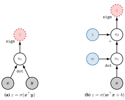
2.1 Two simple computation graphs with inputs (gray), parameters (blue), intermediate variablesui, and outputs (dashed). Operations are shown next to the nodes. . . 31 2.2 Computation graph forz =_kC1_i+P1_s₋C1_j_k1. . . 31

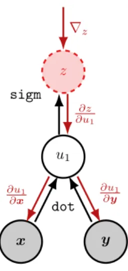
2.3 Backward pass for the computation graph shown in Fig. 2.1a. . . 33 2.4 Simplified pseudocode for symbolic backward chaining (cycle

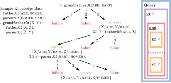
de-tection omitted for brevity, see Russell and Norvig [2010], Gelder [1987], Gallaire and Minker [1978] for details). . . 36 2.5 Full proof tree for a small knowledge base. . . 37 2.6 Knowledge base inference as matrix completion with true training

facts (green), unobserved facts (question mark), relation representa-tions (red), and entity pair representarepresenta-tions (orange). . . 41 2.7 A complete computation graph of a single training example for

Bayesian personalized ranking with`2-regularization. . . 42

3.1 Computation graph for rule in Eq. 3.7 where_·denotes a placeholder for the output of the connected node. . . 51 3.2 Given a set of training ground atoms, matrix factorization learns

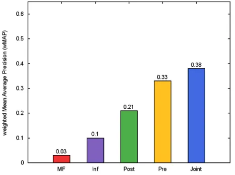
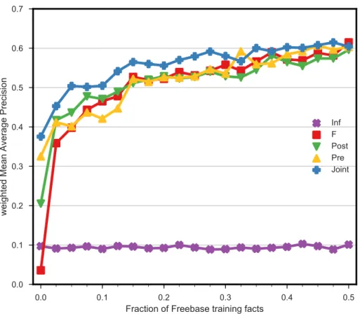
k-dimensional predicate and constant pair representations. Here, we also consider additional first-order logic rules (red) and seek to learn symbol representations such that the predictions (completed matrix) comply with these given rules. . . 53 3.3 Weighted MAP scores for zero-shot relation learning. . . 58 3.4 Weighted MAP of the various models as the fraction of Freebase

training facts is varied. For0% Freebase training facts we get the zero-shot relation learning results presented in Table 3.2. . . 59 3.5 Precision-recall curve demonstrating that theJointmethod, which

incorporates annotated rules derived from the data, outperforms existing factorization approaches (MFandRiedel13-F). . . 61

(18)

4.1 Example for implications that are directly captured in a vector space. 67

4.2 Weighted MAP for injecting rules as a function of the fraction of Freebase facts. . . 72

5.1 A module is mapping an upstream proof state (left) to a list of new proof states (right), thereby extending the substitution set SΨ and

adding nodes to the computation graph of the neural network Sτ representing the proof success. . . 79

5.2 Exemplary construction of an NTP computation graph for a toy knowledge base. Indices on arrows correspond to application of the respective KB rule. Proof states (blue) are subscripted with the sequence of indices of the rules that were applied. Underlined proof states are aggregated to obtain the final proof success. Boxes visualize instantiations of modules (omitted for unify). The proofs S33, S313andS323fail due to cycle-detection (the same rule cannot

be applied twice). . . 84

5.3 Overview of different tasks in the Contries dataset as visualized by Nickel et al. [2016]. The left part (a) shows which atoms are removed for each task (dotted lines), and the right part (b) illustrates the rules that can be used to infer the location of test countries. For taskS1, only facts corresponding to the blue dotted line are removed from the training set. For taskS2, additionally facts corresponding to the green dashed line are removed. Finally, for taskS3also facts for the red dash-dotted line are removed. . . 89

6.1 Computation graph for the fully-connected RNN cell. . . 97

6.2 Computation graph for the LSTM cell. . . 99

6.3 Independent encoding of the premise and hypothesis using the same LSTM. Note that both sentences are compressed as dense vectors as indicated by the red mapping. . . 100

6.4 Conditional encoding with two LSTMs. The first LSTM encodes the premise, and then the second LSTM processes the hypothesis conditioned on the representation of the premise (s5). . . 102

(19)

6.5 Attention model for RTE. Compared to Fig. 6.4, this model does not have to represent the entire premise in its cell state, but can instead output context representations (informally visualized by the red mapping) that are later queried by the attention mechanism (blue). Also note that nowh1 toh5 are used. . . 103

6.6 Word-by-word attention model for RTE. Compared to Fig. 6.5, query-ing the memoryY multiple times allows the model to store more fine-grained information in its output vectors when processing the premise. Also note that now alsoh6toh8are used. . . 105

6.7 Attention visualizations. . . 109 6.8 Word-by-word attention visualizations. . . 113 6.9 Bidirectional encoding of a tweet conditioned on bidirectional

en-coding of a target ([s→

3 s

←

1 ]). The stance is predicted using the last

forward and reversed output representations ([h→

9 h

←

(20)

(21)

List of Tables

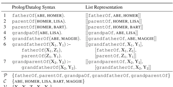
2.1 Example knowledge base using Prolog syntax (left) and as list repre-sentation as used in the backward chaining algorithm (right). . . 34 2.2 Example proof using backward chaining. . . 37

3.1 Top rules for five different Freebase target relations. These im-plications were extracted from the matrix factorization model and manually annotated. The premises of these implications are shortest paths between entity arguments in dependency tree, but we present a simplified version to make these patterns more readable. See Appendix A for the list of all annotated rules. . . 56 3.2 (Weighted) MAP with relations that do not appear in any of the

annotated rules omitted from the evaluation. The difference between PreandJointis significant according to the sign-test (p < 0.05). . . 58 4.1 Weighted MAP for our reimplementation of the matrix factorization

model (F), compared to restricting the constant embedding space (FS) and to injecting WordNet rules (FSL). The orginial matrix factorization model by Riedel et al. [2013] is denoted asRiedel13-F. 70 4.2 Average score of facts with constants that appear in the body of facts

(ei, ej) or in the head (ˆei,eˆj) of a rule. . . 73 5.1 AUC-PR results on Countries and MRR and HITS@mon Kinship,

Nations, and UMLS. . . 91

(22)

(23)

Introduction

“We are attempting to replace symbols by vectors so we can replace logic by algebra.”

— Yann LeCun

The vast majority of knowledge produced by mankind is nowadays available in a digital but unstructured form such as images or text. It is hard for algorithms to extract meaningful information from such data resources, let alone to reason with it. This issue is becoming more severe as the amount of unstructured data is growing very rapidly.

In recent years, remarkable successes in processing unstructured data have been achieved by representation learning methods which automatically learn abstractions from large collections of training data. This is achieved by processing input data using artificial neural networks whose weights are adapted during training. Representation learning lead to breakthroughs in applications such as automated Knowledge Base (KB) completion [Nickel et al., 2012, Riedel et al., 2013, Socher et al., 2013, Chang et al., 2014, Yang et al., 2015, Neelakantan et al., 2015, Toutanova et al., 2015, Trouillon et al., 2016], as well as Natural Language Processing (NLP) applications like paraphrase detection [Socher et al., 2011, Hu et al., 2014, Yin and Sch¨utze, 2015], machine translation [Bahdanau et al., 2014], image captioning [Xu et al., 2015], speech recognition [Chorowski et al., 2015] and sentence summarization [Rush et al., 2015], to name just a few.

Representation learning methods achieve remarkable results, but they usually rely on a large amount of annotated training data. Moreover, since representation learning operates on a subsymbolic level (for instance by replacing words with lists of real numbers – so-called vector representations or embeddings), it is hard to determine why we obtain a certain prediction, let alone how to correct systematic errors or how to incorporate domain and commonsense knowledge. In fact, a recent General Data Protection Regulation by the European Union introduces the “right

(24)

to explanation” of decisions by algorithms and machine learning models that affect users [Council of the European Union, 2016], to be enacted in 2018. This has profound implications for the future development and research of machine learning algorithms [Goodman and Flaxman, 2016], especially for nowadays commonly used representation learning methods. Moreover, for many domains of interests there is not enough annotated training data, which renders applying recent representation learning methods difficult.

Many of these issues do not exist with purely symbolic approaches. For instance, given a KB of facts and first-order logic rules, we can use Prolog to obtain an answer as well as a proof for a query to this KB. Furthermore, we can easily incorporate domain knowledge by adding more rules. However, rule-based system do not generalize to new questions. For instance, given that an apple is a fruit and apples are similar to oranges, we would like to infer that oranges are likely also fruits.

To summarize, symbolic rule-based systems are interpretable and easy to modify. They do not need large amounts of training data and we can easily incorporate domain knowledge. On the other hand, learning subsymbolic representations requires a lot of training data. The trained models are generally opaque and it is hard to incorporate domain knowledge. Consequently, we would like to develop methods that take the best of both worlds.

1.1 Aims

In this thesis, we are investigating the combination of representation learning with first-order logic rules and reasoning. Representation learning methods achieve strong generalization by learning subsymbolic vector representations that can capture similarity and even logical relationships directly in a vector space [Mikolov et al., 2013]. Symbolic representations, on the other hand, allow us to formalize domain and commonsense knowledge using rules. For instance, we can state that everyhuman ismortal, or that everygrandfatheris afatherof aparent. Such rules are often worth many training facts. Furthermore, by using symbolic representations we can take advantage of algorithms for multi-hop reasoning like Prolog’s backward chaining algorithm [Colmerauer, 1990]. Backward chaining is not only widely used for multi-hop question answering in KBs, but it also provides us with proofs in addition to the answer for a question. However, such symbolic reasoning is relying on a complete specification of background and commonsense knowledge in logical form. As an example, let us assume we are asking for thegrandpaof a person, but only know thegrandfatherof that person. If there is no explicit rule connecting grandpatograndfather, we will not find an answer. However, given a large

(25)

KB, we can use representation learning to learn thatgrandpaandgrandfather mean the same thing, or that alecturer is similar to a professor [Nickel et al., 2012, Riedel et al., 2013, Socher et al., 2013, Chang et al., 2014, Yang et al., 2015, Neelakantan et al., 2015, Toutanova et al., 2015, Trouillon et al., 2016]. This becomes more relevant once we do not only want to reason with structured relations but also use textual patterns as relations [Riedel et al., 2013].

The problem that we seek to address in this thesis is how symbolic logical knowledge can be combined with representation learning to make use of the best of both worlds. Specifically, we investigate the following research questions.

• Can we efficiently incorporate domain and commonsense knowledge in form of rules into representation learning methods?

• Can we use rules to alleviate the need for large amounts of training data while still generalizing beyond what is explicitly stated in these rules?

• Can we synthesize representation learning with symbolic multi-hop reasoning as used for automated theorem proving?

• Can we learn rules directly from data using representation learning?

• Can we determine the logical relationship between natural language sentences using representation learning?

1.2 Contributions

This thesis makes the following core contributions.

Regularizing Representations by First-order Logic RulesWe introduce a method for incorporating function-free first-order logic rules directly into vector representa-tions of symbols, which avoids the need for symbolic inference. Instead of symbolic inference, we regularize symbol representations by given rules such that logical rela-tionships hold implicitly in the vector space (Chapter 3). This is achieved by mapping propositional logical rules to differentiable loss terms so that we can calculate the gradient of a given rule with respect to symbol representations. Given a first-order logic rule, we stochastically ground free variables using constants in the domain, and add the resulting loss term for the propositional rule to the training objective of a neural link prediction model for automated KB completion. This allows us to infer relations with little or no training facts in a KB. While mapping logical rules to soft rules using algebraic operations has a long tradition (e.g. in Fuzzy logic), our contribution is the connection to representation learning, i.e., using such rules to

(26)

directly learning better vector representations of symbols that can be used to improve performance on a downstream task such as automated KB completion. Content in this chapter first appeared in the following two publications:

Tim Rockt¨aschel, Matko Bosnjak, Sameer Singh and Sebastian Riedel. 2014. Low-Dimensional Embeddings of Logic. In Proceedings of Association for Computational Linguistics Workshop on Semantic Parsing (SP’14).

Tim Rockt¨aschel, Sameer Singh and Sebastian Riedel. 2015. Injecting Logical Background Knowledge into Embeddings for Relation Extraction. In Pro-ceedings of North American Chapter of the Association for Computational Linguistics – Human Language Technologies (NAACL HLT 2015).

Lifted Regularization of Predicate Representations by ImplicationsFor the sub-class of first-order logic implication rules, we present a scalable method that is independent of the size of the domain of constants, that generalizes to unseen con-stants, and that can be used with a broader class of training objectives (Chapter 4). Instead of relying on stochastic grounding, we use implication rules directly as regularizers for predicate representations. Compared to the method in Chapter 3, this method is independent of the number of constants and ensures that a given implication between two predicates holds for any possible pair of constants at test time. Our method is based on Order Embeddings [Vendrov et al., 2016] and our contribution is the extension to the task of automated KB completion which requires constraining entity representations to be non-negative. This chapter is based on the following two publications:

Thomas Demeester, Tim Rockt¨aschel and Sebastian Riedel. 2016. Regularizing Relation Representations by First-order Implications. InProceedings of North American Chapter of the Association for Computational Linguistics (NAACL) Workshop on Automated Knowledge Base Construction (AKBC).

Thomas Demeester, Tim Rockt¨aschel and Sebastian Riedel. 2016. Lifted Rule Injection for Relation Embeddings. InProceedings of Empirical Methods in Natural Language Processing (EMNLP).

My contribution to this work is the conceptualization of the model, the design of experiments, and the extraction of commonsense rules from WordNet.

End-to-end Differentiable ProvingCurrent representation learning and neural link prediction models have deficits when it comes to complex multi-hop inferences such as transitive reasoning [Bouchard et al., 2015, Nickel et al., 2016]. Automated theorem provers, on the other hand, have a long tradition in computer science and

(27)

provide elegant ways to reason with symbolic knowledge. In Chapter 5, we propose Neural Theorem Provers (NTPs): end-to-end differentiable theorem provers for automated KB completion based on neural networks that are recursively constructed and inspired by Prolog’s backward chaining algorithm. By doing so, we can calculate the gradient of a proof success with respect to symbol representations in a KB. This allows us to learn symbol representations directly from facts in a KB, and to make use of the similarities of symbol representations and provided rules in proofs. In addition, we demonstrate that we can induce interpretable rules of predefined structure. On three out of four benchmark KBs, our method outperforms ComplEx [Trouillon et al., 2016], a state-of-the-art neural link prediction model. Work in this chapter appeared in:

Tim Rockt¨aschel and Sebastian Riedel. 2016. Learning Knowledge Base Inference with Neural Theorem Provers. In Proceedings of North American Chapter of the Association for Computational Linguistics (NAACL) Workshop on Automated Knowledge Base Construction (AKBC).

Tim Rockt¨aschel and Sebastian Riedel. 2017. End-to-End Differentiable Proving. InAdvances in Neural Information Processing Systems 31: Annual Conference on Neural Information Processing Systems (NIPS).

Recognizing Textual Entailment with Recurrent Neural Networks Representa-tion learning models such as Recurrent Neural Networks (RNNs) can be used to map natural language sentences to fixed-length vector representations, which has been successfully applied for various downstream NLP tasks including Recognizing Textual Entailment (RTE). In RTE, the task is to determine the logical relationship between two natural language sentences. This has so far been either approached by NLP pipelines with hand-crafted features, or neural network architectures that independently map the two sentences to fixed-length vector representations. Instead of encoding the two sentences independently, we propose a model that encodes the second sentence conditioned on an encoding of the first sentence. Furthermore, we apply a neural attention mechanism to bridge the hidden state bottleneck of the RNN (Chapter 6). Work in this chapter first appeared in:

Tim Rockt¨aschel, Edward Grefenstette, Karl Moritz Hermann, Tomas Kocisky and Phil Blunsom. 2016. Reasoning about Entailment with Neural Attention. In Proceedings of International Conference on Learning Representations (ICLR).

(28)

1.3 Thesis Structure

In Chapter 2, we provide background on representation learning, computation graphs, first-order logic, and the notation used throughout the thesis. Furthermore, we explain the task of automated KB completion and describe neural link prediction and path-based approaches that have been proposed for this task. Chapter 3 introduces a method for regularizing symbol representations by first-order logic rules. In Chapter 4, we subsequently focus on direct implications between predicates, a subset of first-order logic rules. For this class of rules, we provide an efficient method by directly regularizing predicate representations. In Chapter 5, we introduce a recursive construction of a neural network for automated KB completion based on Prolog’s backward chaining algorithm. Chapter 6 presents a RNN for RTE based on conditional encoding and a neural attention mechanism. Finally, Chapter 7 concludes the thesis with a discussion of limitations, open issues, and future research avenues.

(29)

Background

This chapter introduces core methods used in the thesis. Section 2.1 explains function approximation with neural networks and backpropagation. Subsequently, Section 2.2 introduces function-free first-order logic, the backward chaining algorithm, and inductive logic programming. Finally, Section 2.3 discusses prior work on automated knowledge base completion, linking the first two sections together.

2.1 Function Approximation with Neural Networks

In this thesis, we consider models that can be formulated as differentiable func-tionsfθ : _{X → Y} parameterized byθ_∈Θ. Our task is to find such functions,i.e., to learn parametersθfrom a set of training examples_T =_{(xi, yi)_}wherexi _{∈ X} is the input andyi _{∈ Y} some desired output of theith training example. Both,xiand yi, can be structured objects. For instance,xicould be a fact about the world, like directedBy(INTERSTELLAR,NOLAN), andyia corresponding target truth score

(e.g. 1.0for TRUE).

We define a loss function_L: Y × Y ×Θ→Rthat measures the discrepancy between a provided outputy and a predicted outputfθ(x)on an inputx, given a current setting of parametersθ. We seek to find those parametersθ∗

that minimize this discrepancy on a training set. We denote the global loss over the entire training data asL. Our learning problem can thus be written as

θ∗ = arg min θ L= arg min θ 1 |T | X (x,y)∈ T L(fθ(x), y,θ). (2.1) Note that_Lis also a function ofθ, since we might not only want to measure the discrepancy between given and predicted outputs, but also use a regularizer on the parameters to improve generalization. Sometimes, we omitθin_Lfor brevity. As_L andfθ are differentiable functions, we can use gradient-based optimization methods,

(30)

such as Stochastic Gradient Descent (SGD) [Nemirovski and Yudin, 1978], for iteratively updatingθbased on mini-batches_{B ⊆ T} of the training data1

θt+1 =θt−η∇θt 1 |B| X (x,y)∈ B L(fθ(x), y,θt) (2.2)

whereηdenotes a learning rate, and_∇θ denotes the differentiation operation of the loss with respect to parameters, given the current batch at time stept.

2.1.1 Computation Graphs

A useful abstraction for defining models as differentiable functions arecomputation graphs which illustrate the computations carried out by a model more precisely [Goodfellow et al., 2016]. In such a directed acyclic graph, nodes represent variables and directed edges from one or multiple nodes to another node correspond to a differentiable operation. As variables we consider scalars, vectors, matrices, and, more generally, higher-order tensors.2 _{We denote scalars by lower case letters}_x,

vectors by bold lower case lettersx, matrices by bold capital lettersX, and higher-order tensors by Euler script letters_X. Variables can either be inputs, outputs, or parameters of a model.

Figure 2.1a shows a simple computation graph that calculates z = σ(x>_y_). Here,σandsigmrefer to the element-wise (or scalar) sigmoid operation

σ(x) = 1

1 +e−x (2.3)

and dotandx>_y_{denote the dot product between two vectors. Furthermore, we} name the ith intermediate expression as ui. Figure 2.1b shows a slightly more complex computation graph with two parameterswandb. This computation graph in fact represents logistic regressionf(x) = σ(w>_x₊_b).

2.1.2 From Symbols to Subsymbolic Representations

In this thesis, we will use neural networks to learn representations of symbols. For instance, such symbols can be words, constants, or predicate names. When we say we learn a subsymbolic representation for symbols, we mean that we map symbols to fixed-dimensional vectors or more generally tensors. This can be done by first

1_{Note that there are many alternative methods for minimizing the loss in Eq. 2.1, but all models in}

this thesis are optimized by variants of SGD.

2_{For implementation purpose we will also consider structured objects over such tensors, like tuples}

and lists. Current deep learning libraries such as Theano [Al-Rfou et al., 2016], Torch [Collobert et al., 2011] and TensorFlow [Abadi et al., 2016] come with support for tuples and lists. However, for brevity we leave them out of the description here.

(31)

x y u1 dot z sigm (a)z=σ(x>_y₎ x u1 w dot u2 b + z sigm (b)z=σ(w>_x₊_b₎

Figure 2.1:Two simple computation graphs with inputs (gray), parameters (blue), inter-mediate variablesui, and outputs (dashed). Operations are shown next to the

nodes. 1s 1i 1j vs vi vj P C u1 u2 z

matmul matmul matmul

+

− k•k₁

Figure 2.2:Computation graph forz=_kC1i+P1s−C1jk1.

enumerating all symbols and then assigning the numberito the ith symbol. Let

S be the set of all symbols. We denote the one-hot vector for the ith symbol as

1i ∈ {0,1}|S|, which is1 at index iand 0 everywhere else. Figure 2.2 shows a computation graph whose inputs are one-hot vectors of some symbols with indices s, i, and j. In the first layer, these one-hot vectors are mapped to dense vector

(32)

representations via a matrix multiplication with so-called embedding lookup matrices (P andC in this case).

This computation graph corresponds to a neural link prediction model that we explain in more detail in Section 2.3.2. Here it serves only as an illustration for how symbols can be mapped to vector representations. In the remainder of this thesis, we will often omit the embedding layer for clarity. The goal is to learn symbol representations such asvs,viandvj automatically from data. To this end, we need to be able to calculate the gradient of the output of the computation graph with respect to its parameters (the embedding lookup matrices in this case).

2.1.3 Backpropagation

For learning from data, we need to be able to calculate the gradient of a loss with respect to all model parameters. As we assume all operations in the computation graph are differentiable, we can recursively apply the chain rule of calculus.

Chain Rule of CalculusAssume we are given a composite functionz =f(y) = f(g(x)) with f : Rn _→ _Rm _and _g _: _Rl _→ _Rn_{. The chain rule allows us to} decompose the calculation of _∇xz,i.e., the gradient of the entire computation z with respect tox, as follows [Goodfellow et al., 2016]

∇xz = ∂y ∂x > ∇yz. (2.4)

Here, ∂y_∂x is the Jacobian matrix ofg,i.e., the matrix of partial derivatives, and_∇yz is the gradient ofzwith respect toy. Note that this approach generalizes to matrices and higher-order tensors by reshaping them to vectors before the gradient calculation (vectorization) and back to their original shape afterwards.

Backpropagation uses the chain rule to recursively define the efficient calcula-tion of gradients of parameters (and inputs) in the computacalcula-tion graph by avoiding recalculation of previously calculated expressions. This is achieved via dynamic programming,i.e., storing previously calculated gradient expressions and reusing them for later gradient calculations. We refer the reader to Goodfellow et al. [2016] for details. In order to run backpropagation with a differentiable operationf that we want to use in a computation graph, all we need to ensure is that this function is differentiable with respect to each one of its inputs.

ExampleLet us take the computation graph depicted in Fig. 2.1a as an example. Assume we are given an upstream gradient_∇zand want to compute the gradient ofz with respect to the inputsxandy. The computations carried out by backpropagation

(33)

x y u1 dot z sigm ∇z ∂z ∂u1 ∂u1 ∂x ∂u1 ∂y

Figure 2.3:Backward pass for the computation graph shown in Fig. 2.1a.

are depicted in Fig. 2.3. For instance, by recursively applying the chain rule we can calculate_∇xzas follows: ∇xz = ∂z ∂x = ∂z ∂u1 ∂u1 ∂x =σ(u1)(1−σ(u1))y. (2.5)

Note that the computation of _∂u1∂z can be reused for calculating _∇yz. We get the gradient of the entire computation graph (including upstream nodes) with respect toxvia _∇z∇xz. Later we will use computation graphs where nodes are used in multiple downstream computations. Such nodes receive multiple gradients from downstream nodes during backpropagation, which are summed up to calculate the gradient of the computation graph with respect to the variable represented by the node.

In Chapter 3, we will use backpropagation for computing the gradient of differ-entiable propositional logic rules with respect to vector representations of symbols to develop models that combine representation learning with first-order logic. In Chapter 5, we take this further and construct a computation graph for all possible proofs in a Knowledge Base (KB) using the backward chaining algorithm. This will allow us to calculate the gradient of proofs with respect to symbol representations and to induce rules using gradient descent. Finally, in Chapter 6, we will use Recurrent Neural Networks (RNNs),i.e., computation graphs that are dynamically constructed for input varying-length input sequences of word representations.

(34)

Prolog/Datalog Syntax List Representation

1 fatherOf(ABE,HOMER). [[fatherOf,ABE,HOMER]]

2 parentOf(HOMER,LISA). [[parentOf,HOMER,LISA]]

3 parentOf(HOMER,BART). [[parentOf,HOMER,BART]]

4 grandpaOf(ABE,LISA). [[grandpaOf,ABE,LISA]]

5 grandfatherOf(ABE,MAGGIE). [[grandfatherOf,ABE,MAGGIE]]

6 grandfatherOf(X1,Y1):– [[grandfatherOf,X1,Y1],

fatherOf(X1,Z1), [fatherOf,X1,Z1],

parentOf(Z1,Y1). [parentOf,Z1,Y1]]

7 grandparentOf(X2,Y2):– [[grandparentOf,X2,Y2],

grandfatherOf(X2,Y2). [grandfatherOf,X2,Y2]]

P {fatherOf,parentOf,grandpaOf,grandfatherOf,grandparentOf}

C {ABE,HOMER,LISA,BART,MAGGIE}

V {X1,Y1,Z1,X2,Y2}

Table 2.1:Example knowledge base using Prolog syntax (left) and as list representation as used in the backward chaining algorithm (right).

2.2 Function-free First-order Logic

We now turn to a brief introduction of function-free first-order logic to the extent it is used in subsequent chapters. This section follows the syntax of Prolog and Datalog [Gallaire and Minker, 1978], and is based on Lloyd [1987], Nilsson and Maluszynski [1990], and Dzeroski [2007].

2.2.1 Syntax

We start by defining anatomas apredicate3 _{symbol and a list of terms. We will}

use lowercase names to refer to predicate and constant symbols (e.g. fatherOf and BART), and uppercase names for variables (e.g. X, Y, Z). In Prolog, one also considers function terms and defines constants as function terms with zero arity. However, in this thesis we will work only with function-free first-order logic rules, the subset of logic that Datalog supports. Hence, for us a term can be a constant or a variable. For instance,grandfatherOf(Q,BART)is an atom with

the predicategrandfatherOf, and two terms, the variable Q and the constant

BART, respectively. We define thearityof a predicate to be the number of terms

it takes as arguments. Thus, grandfatherOf is a binary predicate. A literal is defined as a negated or non-negated atom. Aground literalis a literal with no variables (see rules1to5in Table 2.1). Furthermore, we consider first-order logic rules4of the form H :–B, where the bodyB(also called condition or premise) is a possibly empty conjunction of atoms represented as a list, and the head H (also

3_{We will use predicate and relation synonymously throughout this thesis.} 4_{We will use rule, clause and formula synonymously.}

(35)

called conclusion, consequent or hypothesis) is an atom. Examples are rules6and 7in Table 2.1. Such rules with only one atom as the head are calleddefinite rules. In this thesis we only consider definite rules. Variables are universally quantified (e.g._∀X1,Y1,Z1in rule6). A rule is a ground rule if all its literals are ground. We

call a ground rule with an empty body afact, hence the rules1 to5 in Table 2.1 are facts.5 _{We define}_S ₌_{C ∪ P ∪ V} _{to be the set of symbols, containing constant}

symbols_C, predicate symbols_P, and variable symbols_V. We call a set of definite rules like the one in Table 2.1 aknowledge baseorlogic program. Asubstitution Ψ =_{X1/t1, . . . ,XN/tN}is an assignment of variable symbols Xi to termsti, and applying a substitution to an atom replaces all occurrences of variables Xiby their respective termti.

What we have defined so far is the syntax of logic used in this thesis. To assign meaning to this language (semantics), we need to be able to derive the truth value for facts. We focus on proof theory,i.e., deriving the truth of a fact from other facts and rules in a KB.6_{In the next subsection we explain backward chaining, an algorithm}

for deductive reasoning. It is used to derive atoms from other atoms by applying rules.

2.2.2 Deduction with Backward Chaining

Representing knowledge (facts and rules) in symbolic form has the appeal that one can use automated deduction systems to infer new facts. For in-stance, given the logic program in Table 2.1, we can automatically deduce that grandfatherOf(ABE,LISA)is a true fact by applying rule 6 using facts 1 and 2.

Backward chaining is a common method for automated theorem proving, and we refer the reader to Russell and Norvig [2010], Gelder [1987], Gallaire and Minker [1978] for details and to Fig. 2.4 for an excerpt of the pseudocode in style of a functional programming language. Particularly, we are making use of pattern matching to check for properties of arguments passed to a module. Note that ” ” matches every argument and that the order matters,i.e., if arguments match a line, subsequent lines are not evaluated. We denote sets by Euler script letters (e.g. _E), lists by small capital letters (e.g. E), lists of lists by blackboard bold letters (e.g. E) and we use:to refer to prepending an element to a list (e.g.e :E or E:E). While an atom is a list of a predicate symbol and terms, a rule can be seen as a list of atoms and thus a list of lists where the head of the list is the rule head.7

5_{We sometimes only call a rule a rule if it has a non-empty body. This will be clear from the}

context.

6_{See Dzeroski [2007] for other methods for semantics.}

(36)

1. or(G, S) =[S0_|S0 _∈and(B,unify(H,G, S))for H :–B_∈K]

2. and( ,FAIL) =FAIL 3. and([ ], S) =S

4. and(G:G, S) =[S00 |S00∈and(G, S0)forS0 ∈or(substitute(G, S), S)]

5. unify( , ,FAIL) =FAIL 6. unify([ ],[ ], S) = S 7. unify([ ], , ) = FAIL 8. unify( ,[ ], ) = FAIL 9. unify(h: H, g :G, S) = unify     H,G,        S∪ {h/g} ifh∈ V S_{∪ {}g/h_} ifg _{∈ V}, h_{6∈ V} S ifg =h FAIL otherwise            10. substitute([ ], ) = [ ] 11. substitute(g :G, S) = x ifg/x_∈S g otherwise :substitute(G, S)

Figure 2.4:Simplified pseudocode for symbolic backward chaining (cycle detection omitted for brevity, see Russell and Norvig [2010], Gelder [1987], Gallaire and Minker [1978] for details).

Given a goal such as grandparentOf(Q1,Q2), backward chaining

finds substitutions of free variables with constants in facts in a KB (e.g.

{Q₁/ABRAHAM,Q₂/BART}). This is achieved by recursively iterating through rules that translate a goal into subgoals which we attempt to prove, thereby exploring possible proofs. For example, the KB could contain the following rule that can be applied to find answers for the above goal:

grandfatherOf(X,Y):–fatherOf(X,Z),parentOf(Z,Y).

The proof exploration in backward-chaining is divided into two functions called or and and that perform a depth-first search through the space of possible proofs. The function or (line 1) attempts to prove a goal by unifying it with the head of every rule in a KB, yielding intermediate substitutions. Unification (lines 5-9) iterates through pairs of symbols in the two lists corresponding to the atoms that we want to unify and updates the substitution set if one of the two symbols is a variable. It

(37)

Rule Remaining Goals S

[[grandparentOf,Q1,Q2]] { }

7 [[grandfatherOf,Q1,Q2]] {X2/Q1,Y2/Q2}

6 [[fatherOf,Q1,Z1],[parentOf,Z1,Q2]] {X2/Q1,Y2/Q2,X1/Q1,Y1/Q2}

1 [[parentOf,HOMER,Q2]] {X2/Q1,Y2/Q2,X1/Q1,Y1/Q2,Q1/ABE,Z1/HOMER}

2 [ ] {X2/Q1,Y2/Q2,X1/Q1,Y1/Q2,Q1/ABE,Z1/HOMER,Q2/LISA} Table 2.2: Example proof using backward chaining.

Example Knowledge Base: 1. fatherOf(abe,homer).

2. parentOf(homer,bart).

3. grandfatherOf(X,Y):– fatherOf(X,Z),

parentOf(Z,Y).

?–grandfatherOf(abe,bart).

failure failure success

{X/abe,Y/bart}

3.1 ?–fatherOf(abe,Z).

1 2 3

success

{X/abe,Y/bart,Z/homer}

3.2 ?–parentOf(bart,homer).

failure failure

1 2 3

failure success

{X/abe,Y/bart,Z/homer} failure 1 2 3 Query or 1 and1 or 2 or 2

Figure 2.5:Full proof tree for a small knowledge base.

returns a failure if two non-variable symbols are not identical or the two atoms have different arity. For rules where unification with the head of the rule succeeds, the body and substitution are passed to and (lines 2-4), which then attempts to prove every atom in the body sequentially by first applying substitutions and subsequently calling or. This is repeated recursively until unification fails, atoms are proven by unification via grounding with facts in the KB, or a certain proof-depth is exceeded. Table 2.2 shows a proof for the querygrandparentOf(Q1,Q2)given the KB in

Table 2.1 using Fig. 2.4. The method substitute (lines 10-11) replaces variables in an atom by the corresponding symbol if there exists a substitution for that variable in the substitution list. Figure 2.5 shows the full proof tree for a small knowledge base and the query ?–grandfatherOf(ABE,BART).8 The numbers on the arrows correspond to the application of the respective rules. We visualize the recursive calls to or and and together with the proof depth on the right side. Note how most proofs can be aborted early due to unification failure.

Though first-order logic can be used for complex multi-hop reasoning, a draw-back is that for such symbolic inference there is no generalization beyond what we explicitly specify in the facts and rules. For instance, given a large KB we would

(38)

like to learn automatically that in many cases where we observefatherOf we also observeparentOf. This can be approached by statistical relational learning, inductive logic programming, and particularly neural networks for KB completion which we discuss in the remainder of this chapter.

2.2.3 Inductive Logic Programming

While backward chaining is used fordeduction,i.e., for inferring facts given rules and other facts in a KB, Inductive Logic Programming (ILP) [Muggleton, 1991] combines logic programming with inductive learning to learn logic programs from training data. This training data can include facts, but also a provided logic program that the ILP system is supposed to extend. Specifically, given facts and rules, the task of an ILP system is to find further regularities and form hypotheses for unseen facts [Dzeroski, 2007]. Crucially, these hypothesis are again formulated using first-order logic.

There are different variants of ILP learning tasks [Raedt, 1997] and we focus onlearning from entailment[Muggleton, 1991]. That is, given examples of positive facts and negative facts, the ILP system is supposed to find rules such that positive facts can be deduced, but negative facts cannot. There are many variants of ILP systems, and we refer the reader to Muggleton and Raedt [1994] and Dzeroski [2007] for an overview. One of the most prominent systems is the First Order Inductive Learner (FOIL) [Quinlan, 1990], which is a greedy algorithm that induces one rule at a time by constructing a body that satisfies the maximum number of positive facts and the minimum number of negative facts.

In Chapter 5, we will construct neural networks for proving facts in a KB and introduce a method for inducing logic programs using gradient descent while learning vector representations of symbols.

2.3 Automated Knowledge Base Completion

Automated KB completion is the task of inferring facts from information contained in a KB and other resources such as text. This is an important task as real-world KBs are usually incomplete. For instance, theplaceOfBirthpredicate is missing for71% of people in Freebase [Dong et al., 2014]. Prominent recent approaches to automated KB completion learn vector representations of symbols via neural link prediction models. The appeal of learning suchsubsymbolicrepresentations lies in their ability to capture similarity and even implicature directly in a vector space. Compared to ILP systems, neural link prediction models do not rely on a combinatorial search over the space of logic programs, but instead learn a local scoring function based on

(39)

subsymbolic representations using continuous optimization. However, this comes at the cost of uninterpretable models and no straightforward ways of incorporating logical background knowledge – drawbacks that we seek to address in this thesis. Another benefit of neural link prediction models over ILP is that inferring whether a fact is true or not often amounts to efficient algebraic operations (feed-forward passes in shallow neural networks), which makes test-time inference very scalable. In addition, representations of symbols can be compositional. For instance, we can compose a representation of a natural language predicate from a sequence of word representations [Verga et al., 2016a].

In recent years, many models for automated KB completion have been proposed. In the next sections, we discuss prominent approaches. On a high level, these methods can be categorized into (i) neural link prediction models which define a local scoring function for the truth of a fact based on estimated symbol representations, and (ii) models that use paths between two entities in a KB for predicting new relations between them.

2.3.1 Matrix Factorization

In this section, we describe the matrix factorization relation extraction model by Riedel et al. [2013], which is an instance of a simple neural link prediction model. We discuss this model in detail, as it the basis on which we develop rule injection methods in Chapter 3 and 4.

Assume a set of observed entity pair symbols _C and a set of predicate sym-bols _P, which can either represent structured binary relations from Freebase, a large collaborative knowledge base [Bollacker et al., 2008], or unstructured Open Information Extraction (OpenIE) [Etzioni et al., 2008] textual surface patterns col-lected from news articles. Examples for structured and unstructured relations are company/founders and #2-co-founder-of-#1, respectively. Here, #2-co-founder-of-#1 is a textual pattern where #1and #2are placehold-ers for entities. For instance, the relationship between Elon Musk and Tesla in the sentence “Elon Musk, the co-founder of Tesla and the CEO of SpaceX, cites The Foundation Trilogy by Isaac Asimov as a major influence on his think-ing”9could be expressed by the ground atom#2-co-founder-of-#1(TESLA,

ELON MUSK). In this example, ELON MUSK appeared first in the textual pattern, but #2 indicates that this constant will be used as the second argument in the predicate corresponding to the pattern. That way we can later introduce a rule

(40)

∀X,Y :company/founders(X,Y):–#2-co-founder-of-#1(X,Y) with-out changing the order of the variables in the body of the rule.

Let_O =_{rs(ei, ej))_}be the set of observed ground atoms. Model F by Riedel et al. [2013] maps all symbols in a knowledge base to subsymbolic representations, i.e., it learns a dense k-dimensional vector representation for every relation and entity pair. Thus, a training factrs(ei, ej)is represented by two vectors, vs ∈ Rk and vij ∈ Rk, respectively. We will refer to these asembeddings, subsymbolic representations,vector representations,neural representations, or simply (symbol) representations when it is clear from the context. The truth estimate of a fact is modeled via the sigmoid of the dot product of the two symbol representations:

psij =σ(vs>vij). (2.6) In fact, this expression corresponds to the computation graph shown in Fig. 2.1a withx=vsandy=vij. The scorepsij is measuring the compatibility between the relation and entity pair representation and can be interpreted as the probability of the fact being true conditioned on parameters of the model. We would like to train symbol representations such that true ground atoms get a score close to one and false ground atoms a score close to zero. This results in a low-rank matrix factorization corresponding to Generalized Principal Component Analysis (GPCA) [Collins et al., 2001]

K _≈σ(P C>) _∈R|P|×|C| (2.7)

where P _∈ R|P|×k _and _C _∈ _R|C|×k _{are matrices of all relation and entity pair} representations, respectively. This factorization is depicted in Fig. 2.6 where known facts are shown in green and the task is to complete this matrix for cells with a question mark. Equation 2.7 leads to generalization with respect to unseen facts as every relation and entity pair is represented in a low-dimensional space, and this information bottleneck will lead to similar entity pairs being represented close in distance in the vector space (likewise for similar predicates).

The distributional hypothesis states that “one shall know a word by the company it keeps” [Firth, 1957]. It has been used for learning word meaning from large collections of text [Lowe and McDonald, 2000, Pad´o and Lapata, 2007]. Applied to automated KB completion, one could say that the meaning of a relation or entity pair can be estimated from the entity pairs and relations that respectively appear together

(41)

#1-is-historian-at-# 2 #1-is-professor-at-# 2 #1-museum-at-#2#1-teaches-history-a t-#2 employeeAt petrie, ucl ferguson, harvard andrew, cambridge trevelyan, cambridge T T T T T T T T ? ? ? ? ? ? ? ? ? ? ? ? vp1 vp2 vp3 vp4 vp5 vc1 vc2 vc3 vc4 ∈Rk

Textual Patterns Freebase

Figure 2.6:Knowledge base inference as matrix completion with true training facts (green), unobserved facts (question mark), relation representations (red), and entity pair representations (orange).

in facts in a KB. That is, if for many entity pairs we observe that bothfatherOf anddadOfis true, we can assume that both relations are similar.

2.3.1.1 Bayesian Personalized Ranking

A common problem in automated KB completion is that we do not observe any negative facts. In the recommendation literature, this problem is called implicit feedback [Rendle et al., 2009]. Applied to KB completion, we would like to infer (or recommend) for a target relation some (unobserved) facts that we do not know from facts that we do know. Facts that we do not know can be unknown either because they are not true or because they are true but missing in the KB.

One method to address this issue is to formulate the problem in terms of a ranking loss, and sample unobserved facts as negative facts during training. Given a known factrs(ei, ej)∈ O, Bayesian Personalized Ranking (BPR) [Rendle et al., 2009] samples another entity pair(em, en)_{∈ C}such thatrs(em, en) _{6∈ O}and adds the soft-constraint

v_s>vij ≥vs>vmn. (2.8) This follows a relaxation of the local Closed World Assumption (CWA) [Gal´arraga et al., 2013, Dong et al., 2014]. In the CWA, the knowledge about true facts

(42)

1s 1ij 1mn

vs vij vmn

matmul matmul matmul

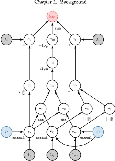
C P u1 u2 dot dot u6 − u8 sigm u10 −log u5 u3 u4 k•k2₂ k•k2₂ k•k2₂ u7 + u9 u11 ∗ ∗ λp λc loss sum

Figure 2.7:A complete computation graph of a single training example for Bayesian per-sonalized ranking with`2-regularization.

for relation rs is assumed to be complete and any sampled unobserved fact can consequently be assumed to be negative. In BPR, the assumption is that unseen facts are not necessarily false but their probability of being true should be less than for known facts. Thus, sampled unobserved facts should have a lower score than known facts. Instead of working with a fixed set of samples, we resample negative facts for every known fact in every epoch, where an epoch is a full iteration through all known facts in a KB. We denote a sample from the set of constant pairs as(em, en)∼ C.10

This leads to the overall approximate loss

L= X rs(ei,ej)∈ O, (em,en)∼ C, rs(em,en)6∈ O −wslogσ(v_s>vij −v>svmn) +λpkvsk22 +λc(kvijk 2 2+kvmnk 2 2) (2.9) 10_{Note that}

(43)

whereλpandλcare the strength of the`2regularization of the relation and entity pair

representations, respectively. Furthermore,wsis a relation-dependent implicit weight accounting for how often(em, en)is sampled during training time. As we resample an unobserved fact every time we visit an observed fact during training, unobserved facts for relations with many observed facts are more likely to be sampled as negative facts than for relations with few observed facts. A complete computation graph of a single training example for matrix factorization using BPR with`2regularization is

shown in Fig. 2.7.

2.3.2

2.3.3 Path-based Models

While all methods presented in the previous section model the truth of a fact as a local scoring function of the representations of the relation and entities (or entity pairs), path-based models score facts based either on random walks over the KBs (path ranking) or by encoding entire paths in a vector space (path encoding).

(45)

2.3.3.1 Path Ranking

The Path Ranking Algorithm (PRA) [Lao and Cohen, 2010, Lao et al., 2011] learns to predict a relation between two entities based on logistic regression over features collected from random walks between these entities in the KB up to some predefined length. Lao et al. [2012] extend PRA inference to OpenIE surface patterns in addition to structured relations contained in KBs.

A related approach to PRA is Programming with Personalized PageRank (ProPPR) [Wang et al., 2013], which is a first-order probabilistic logic program-ming language. It uses Prolog’s Selective Linear Definite clause resolution (SLD) [Kowalski and Kuehner, 1971], a depth-first search strategy for theorem proving, to construct a graph of proofs. Instead of returning deterministic proofs for a given query, ProPPR defines a stochastic process on the graph of proofs using PageRank [Page et al., 1999]. Furthermore, in ProPPR one can use features on the head of rules whose weights are learned from data to guide stochastic proofs. Experiments with ProPPR were conducted on comparably small KBs and contrary to neural link prediction models and the extensions to PRA below, it has not yet been scaled to large real-world KBs [Gardner et al., 2014].

A shortcoming of PRA and ProPPR is that they are operating on symbols instead of vector representations of symbols. This limits generalization as it results in an explosion in the number of paths to consider when increasing the path length. To overcome this limitation, Gardner et al. [2013] extend PRA to include vector representations of verbs. These verb representations are obtained from pre-training via PCA on a matrix of co-occurrences of verbs and subject-object tuples collected from a large dependency-parsing corpus. Subsequently, these representations are used for clustering relations, thus avoiding an explosion of path features in prior PRA work while improving generalization. Gardner et al. [2014] take this approach further by introducing vector space similarity into random walk inference, thus dealing with paths containing unseen surface forms by measuring the similarity to surface forms seen during training, and following relations proportionally to this similarity.

2.3.3.2 Path Encoding

While Gardner et al. introduced vector representations into PRA, these representa-tions are not trained end-to-end from task data but instead pretrained on an external corpus. This means that relation representations cannot be adapted during training on a KB.

Neelakantan et al. [2015] propose RNNs for learning embeddings of entire paths. The input to these RNNs are trainable relation representations. Given a known

(46)

relation between two entities and a path connecting the two entities in the KB, an RNN for the target relation is trained to output an encoding of the path such that the dot product of that encoding and the relation representation is maximal.

Das et al. [2017] note three limitations of the work by Neelakantan et al. [2015]. First, there is no parameter sharing of RNNs that encode different paths for different target relations. Second, there is no aggregation of information from multiple path encodings. Lastly, there is no use of entity information along the path as only relation representations are fed to the RNN. Das et al. address the first issue by using a single RNN whose parameters are shared across all paths. To address the second issue, Das et al. train an aggregation function over the encodings of multiple paths connecting two entities. Finally, to obtain entity representations that are fed into the RNN alongside relation representations they sum learned vector representations of the entity’s annotated Freebase types.

(47)

Regularizing Representations by

First-order Logic Rules

In this chapter, we introduce a paradigm for combining neural link prediction models for automated Knowledge Base (KB) completion (Section 2.3.2) with background knowledge in the form of first-order logic rules. We investigate simple baselines that enforce rules through symbolic inference before and after matrix factorization. Our main contribution is a novel joint model that learns vector representations of relations and entity pairs using both distant supervision and first-order logic rules, such that these rules are captured directly in the vector space of symbol representations. To this end, we map symbolic rules to differentiable computation graphs representing real-valued losses that can be added to the training objective of existing neural link prediction models. At test time, inference is still efficient as only a local scoring function over symbol representations is used and no logical inference is needed. We present an empirical evaluation where we incorporate automatically mined rules into a matrix factorization neural link prediction model. Our experiments demonstrate the benefits of incorporating logical knowledge for Freebase relation extraction. Specifically, we find that joint factorization of distant and logic supervision is efficient, accurate, and robust to noise (Section 3.5). By incorporating logical rules, we were able to train relation extractors for which no or only few training facts are observed.

3.1 Matrix Factorization Embeds Ground Literals

In Section 2.3.1, we introduced matrix factorization as a method for learning rep-resentations of predicates and constant pairs for automated KB completion. In this section, we elaborate on how matrix factorization indeed embeds ground atoms

(48)

in a vector space and lay out the foundation for developing a method that embeds first-order logic rules.

LetF ∈ F denote a rule in a KB. For instance,Fcould be a ground rule without a body (i.e. a fact) like parentOf(HOMER,BART). Furthermore, let JFK denote the probability of this rule being true conditioned on the parameters of the model. For now, we restrictF to ground atoms and discuss ground literals, propositional rules, and first-order rules later. With slight abuse of notation, let J•K _{also denote}

the mapping of predicate or constant symbols (or a pair of constant symbols) to their subsymbolic representation as assigned by the model. Note that this mapping depends on the neural link prediction model. For matrix factorization, _J•K is a

function_{S →} Rkfrom symbols (constant pairs and predicates) tok-dimensional dense vector representations. For RESCAL (see Section 2.3.2),_J•Kmaps constants

toRk and predicates toRk×k. Using this notation, matrix factorization decomposes the probability of a factrs(ei, ej)as

Jrs(ei, ej)_K=σ(_Jrs_K>_Jei, ej_K) = σ(v_s>vij). (3.1)

Training ObjectiveRiedel et al. [2013] used Bayesian Personalized Ranking (BPR) [Rendle et al., 2009] as training objective,i.e., they encouraged the score of known true facts to be higher than unknown facts (Section 2.3.1.1). However, as we will later model the probability of a rule from the probability of ground atoms scored by a neural link prediction model, we need to ensure that all scores are in the interval[0,1]. Instead of BPR, we thus use the negative log-likelihood loss to directly maximize the probability of all rules,including ground atoms, in a KB (we omit`2regularization

for brevity):

L= X

F∈ F

−log(_JFK). (3.2) Therefore, instead of learning to rank facts, we optimize representations to assign a score close to 1.0 to rules (including facts). Our model can thus be seen as generalization of a neural link prediction model to rules beyond ground atoms.

For matrix factorization as neural link prediction model, we are embedding ground atoms in a vector space of predicate and constant pair representations. Next, we will extend this to ground literals and afterwards to propositional and then first-order logic rules.