The dynamic random subgraph model for the clustering
of evolving networks
Rawya Zreik, Pierre Latouche, Charles Bouveyron
To cite this version:
Rawya Zreik, Pierre Latouche, Charles Bouveyron. The dynamic random subgraph model
for the clustering of evolving networks.
Computational Statistics, Springer Verlag, 2016,
<10.1007/s00180-016-0655-5>.
<hal-01122393v3>
HAL Id: hal-01122393
https://hal.archives-ouvertes.fr/hal-01122393v3
Submitted on 3 May 2016
HAL
is a multi-disciplinary open access
archive for the deposit and dissemination of
sci-entific research documents, whether they are
pub-lished or not.
The documents may come from
teaching and research institutions in France or
abroad, or from public or private research centers.
L’archive ouverte pluridisciplinaire
HAL
, est
destin´
ee au d´
epˆ
ot et `
a la diffusion de documents
scientifiques de niveau recherche, publi´
es ou non,
´
emanant des ´
etablissements d’enseignement et de
recherche fran¸cais ou ´
etrangers, des laboratoires
publics ou priv´
es.
The Dynamic Random Subgraph Model for the
Clustering of Evolving Networks
Rawya ZREIK1,2, Pierre LATOUCHE1 and Charles BOUVEYRON2
1 Laboratoire SAMM, EA 4543, Universit´e Paris 1 Panth´eon-Sorbonne
2 Laboratoire MAP5, UMR CNRS 8145, Universit´e Paris Descartes & Sorbonne Paris Cit´e
Abstract
In recent years, many clustering methods have been proposed to extract in-formation from networks. The principle is to look for groups of vertices with homogenous connection profiles. Most of these techniques are suitable for static networks, that is to say, not taking into account the temporal dimension. This work is motivated by the need of analyzing evolving networks where a decom-position of the networks into subgraphs is given. Therefore, in this paper, we consider the random subgraph model (RSM) which was proposed recently to model networks through latent clusters built within known partitions. Using a state space model to characterize the cluster proportions, RSM is then extended in order to deal with dynamic networks. We call the latter the dynamic ran-dom subgraph model (dRSM). A variational expectation maximization (VEM) algorithm is proposed to perform inference. We show that the variational ap-proximations lead to an update step which involves a new state space model from which the parameters along with the hidden states can be estimated using the standard Kalman filter and Rauch-Tung-Striebel (RTS) smoother. Sim-ulated data sets are considered to assess the proposed methodology. Finally, dRSM along with the corresponding VEM algorithm are applied to an original maritime network built from printed Lloyd’s voyage records.
Key words: State space model, variational inference, variational expectation maximization, maritime data.
1. Introduction
Network analysis has become a mature discipline, since the original work of Moreno (1934), which is no longer limited to sociology and is now applied in many areas such as biology (Albert and Barab´asi, 2002; Barab´asi and Oltvai, 2004; Palla et al., 2005), geography (Ducruet, 2013) or history (Rossi et al., 2014). The growing interest in network analysis is explained partly by the strong presence of this type of data in the digital world, and by recent advances in the modeling and the processing of these data. The clustering methods allow in particular clusters of vertices sharing homogeneous connection profiles to be
uncovered. Most methods look for specific structures, so called communities, which exhibit a transitivity property such that nodes of the same community are more likely to be connected (Hofman and Wiggins, 2008). A popular approach for community discovering, though asymptotically biased (Bickel and Chen, 2009), is based on the modularity score given by Girvan and Newman (2002). Alternative methods usually rely on the latent position cluster model (LPCM) of Handcock et al. (2007) which assumes that the links between the vertices depend on their positions in a social latent space.
The stochastic block model (SBM) (Wang and Wong, 1987; Nowicki and Snijders, 2001) is a flexible random graph model which can also characterize communities, but not only. It is based on a probabilistic generalization of the method applied by White et al. (1976) on Sampson’s famous monastery (Fien-berg and Wasserman, 1981). The SBM model assumes that each vertex belongs to a latent group, and that the probability of connection between a pair of ver-tices depends exclusively on their group. Because no assumption is made on the connection probabilities, various types of structures of vertices can be taken into account. While SBM was originally developed to analyze mainly binary networks, many extensions have been proposed since to deal for instance with valued edges (Mariadassou et al., 2010) or to take into account prior informa-tion (Zanghi et al., 2010; Matias and Robin, 2014). In particular, the random subgraph model (RSM) of Jernite et al. (2014) aims at modeling categorical edges using prior knowledge of a partition of the network into subgraphs. These known subgraphs are assumed to be made of latent clusters which have to be inferred. The vertices are then connected with a probability depending only on the subgraphs whereas the edge type is assumed to be sampled conditionally on the latent groups. This model was applied in the original paper to ana-lyze a historical network in merovingian Gaul. Note that other extensions of SBM have focused on looking for overlapping clusters (Airoldi et al., 2008; La-touche et al., 2011). The inference of SBM like models is usually done using variational expectation maximization (VEM) (Daudin et al., 2008), variational Bayes EM (VBEM) (Latouche et al., 2012), or Gibbs sampling (Nowicki and Sni-jders, 2001). Moreover, we emphasize that various strategies have been derived to estimates the number of corresponding clusters using model selection crite-ria (Daudin et al., 2008; Latouche et al., 2012), allocation sampler (Mc Daid et al., 2013), greedy search (Cˆome and Latouche, 2015), or non parametric schemes (Kemp et al., 2006).
Recently, a few attempts have been made to extend the models mentioned previously in order to deal with dynamic networks. The main idea consists in introducing temporal processes in order to characterize the temporal evolution of nodes and edges through time. Thus, Yang et al. (2011) proposed a dynamic version of SBM allowing a node to switch its class at time t+ 1 depending on its state at time t. The switching probabilities are all characterized by a transition matrix. The alternative extension for SBM of Xu and Hero III (2013) focuses on modeling the temporal changes through a state space model and relies on the Kalman filter for inference. Contrary to Yang et al. (2011), Xu and Hero III (2013) treated the edge probabilities as time varying parameters.
In parallel, the mixed membership SBM (MMSBM) of Airoldi et al. (2008), capable of characterizing overlapping clusters, was adapted to deal with dynamic networks by Xing et al. (2010), Ho et al. (2011) and Kim and Leskovec (2013). Moreover, Sarkar and Moore (2005) derived a dynamic version of the LPCM model of Handcock et al. (2007) keeping the transitivity property that nodes which are close in a social latent space should be more likely to connect. Finally, we would like to highlight the work of Dubois et al. (2013) and Heaukulani and Ghahramani (2013). In Dubois et al. (2013) a non homogeneous Poisson process is considered. Thus, contrary to most clustering models for dynamic networks, a continuous time period is taken into account and events, i.e. the creation or removal of an edge, occur one at a time. While models usually focus on modeling the dynamic of networks through the evolution of their latent structures, Heaukulani and Ghahramani (2013) extended the dynamic latent feature model of Foulds et al. (2011) to define how observed social interactions can affect future unobserved latent structures. In the same vein, a dynamic model inspired by SBM was proposed recently by Xu (2015).
In this paper, we aim at modeling dynamic networks with binary or more generally typed edges, for which a partition of the nodes is given. As an example, we will consider an original network, built from printed Lloyd’s voyage records and describing maritime flows between ports where the geographical positions of the ports play an important role. The partition was obtained by associating each port to a region according to its geographical position. Figure 1 presents the evolution of network navigations, for 23 years between October 1985 and October 2008. A (given) partition of the nodes is seen here as a decomposition of the network into known subgraphs that we propose to model using unobserved clusters that have to be inferred from the data in practice. Thus, considering a slightly different version of the original RSM model of Jernite et al. (2014) and relying on a state space model as in Xing et al. (2010), we propose a new random graph model for evolving networks that we call the dynamic RSM (dRSM) model. The model focuses on describing the network dynamic by characterizing the evolution of the cluster proportions within the known subgraphs. A logistic transformation is used to link the hidden states and the clusters proportions, as in Blei and Lafferty (2007a); Ahmed and Xing (2007). The inference of the model is done using a VEM algorithm.
The article is organized as follows. In Section 2, we introduce the dRSM model along with an inference procedure in Section 3. Variational techniques are considered and a model selection criterion is derived. Finally, the methodology is tested on simulated data in Section 4 and on the maritime network built from Lloyd’s data in Section 5.
2. The dynamic random subgraph model
This section presents the context of the work and introduces the dRSM model along with the modeling of its dynamic. The joint distribution associated with the model is also detailed.
1890 1935
1946 1965
Europe−Atlantic
Asia−Pacific
Middle East & Indian Ocean Med & Black Sea
2008
Figure 1: Connections between a subset of 26 ports (from October 1890 to October 2008). Data extracted from Lloyd’s list. The known subgraphs correspond to geographical regions (continents) indicated using colors.
2.1. Context and notations
We consider a set of T networks {G(t)}T
t=1, whereG(t) is a directed graph
observed at time t. Each G(t) is represented by its N ×N adjacency matrix
X(t) where N denotes the number of nodes. The edge X(t)
i,j, describing the
relationship between nodesi and j, is assumed to take its values in{0, . . . C}
such thatXij(t)=cmeans that nodesiandjare linked by a relationship of type cat timet andXij(t)= 0 indicates the absence of relationship between the two nodes at timet. Note that no self loops are considered,i.e. the connection of a node to itself, thusXii(t)= 0, ∀i, t.
Moreover, a partitionP of the network intoS classes of vertices is assumed to be given. We emphasize that the observed partition induces a decomposition of the graph into subgraphs where each class of vertices corresponds to a specific subgraph. To describe the subgraph membership of each vertex, the variable s is introduced. The variable takes its values in {1, . . . S} and is such thatsi
indicates the subgraph of vertex i. In some cases, and in order to clarify the equations, we will also consider the indicator variables yis such that yis = 1
if nodei is in subgraphs, 0 otherwise. Finally, because the vertex ican only belong to a single subgraph, we havePS
s=1yis= 1.
Our goal is to cluster at each timettheN nodes intoKlatent groups with homogeneous connection profiles, i.e. find an estimate of the set Z of latent variables Zik(t) such that Zik(t) = 1 if at time t, the node i belongs to the class
k, and 0 otherwise. Please note thatN, C, P, S and K are all assumed to be
constant over time.
2.2. The model at each timet
As in the original RSM model, the (known) subgraphs are assumed to be built fromK unobserved clusters of vertices, with varying proportions. Thus, each subgraph s has its own mixing proportion vector α(t)s = (α
(t)
s1, . . . , α
(t) sK)
whereα(t)sk is the proportion of clusterkin subgraphsat timetandPK
k=1α (t) sk =
1,∀s, t. The network is then assumed to be generated at each timetas follows.
Each vertex i is first associated to a latent cluster k with a probability depending on its subgraph si. In practice, the variable Z
(t)
i is drawn from a
multinomial distribution of parameterα(t)si: Zi(t)∼ M(1, α(t)si), and thereforePK k=1Z (t) ik = 1. Note thatZ (t)
ik = 1 indicates that vertexibelongs
to clusterkat time t, 0 otherwise.
On the other hand, the type of link between nodesiandj is assumed to be sampled from a multinomial distribution depending on the latent vectorsZi(t) andZj(t): Xij(t)|Zik(t)Zjl(t)= 1∼ M(1,Πkl), with Πkl ∈[0,1]C+1 andP C c=0Π c kl= 1,∀k, l.
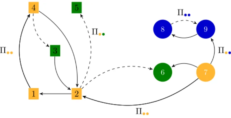
1 2 4 5 3 Π•• Π•• 8 7 6 9 Π•• Π•• Π••
Figure 2: A dRSM network observed at timet. The network is made of 9 nodes belonging
toS= 2 subgraphs (denoted through the form of the nodes) and split intoK = 3 clusters
(indicated by the colors). According to the dRSM model, the directed edges between the
nodes can be of different types (C = 2 types are considered here). Given the clusters, the
presence of an edge depends on the connection probabilities between clusters (Π).
As in the RSM model, and more generally in SBM like models, all vectors Zi(t)are sampled independently, and, conditionally on these membership vectors, the edges are assumed to be independent. Thus, contrary to the original RSM model, the edges depend directly on the latent clusters exclusively, and there is no direct dependency on the subgraphs (see Figure 3). Each edge between a pair (i, j) of vertices does depend on the subgraphssiandsj, but only through
the fact that the edge depends on the latent clusters of the vertices, which themselves depend on the subgraphs. The dependency is indirect while in the original RSM model, the latent clusters along with the subgraphs are all involved in the creation of edges and have different roles. Indeed, the presence or absence of an edge between (i, j) is first drawn from a Bernoulli distribution depending onsi and sj. If an edge is present, the edge type is then sampled depending
on the latent clusters. The separation of roles between the latent clusters and the subgraphs was originally motivated by assumptions regarding the nature of the networks analyzed. We do not make such assumptions in this paper. The latent clusters explain both the creation of an edge and its type.
Figure 2 presents an example of a dRSM network, observed at timet, made of 9 nodes belonging to 2 subgraphs (denoted through the form of nodes) and split into 3 clusters (indicated by the colors).
2.3. Modeling the evolution of random subgraphs
In order to model the evolution of the cluster proportions within the sub-graphs through time, a state space model is considered as in Xing et al. (2010). Thus, the latent variableγs(t)is introduced and a logistic transformationf(·) is
used to link the mixing vectorα(t)s withγ (t) s :
such that α(t)sk =fk(γs(t)) = exp(γ (t) sk −C(γ (t) s )),∀s, k, t,
where γsK(t) = 0 and C(γs(t)) = log(PKk=1exp(γ(t)sk)). The choice to fix the last
component of the vector γs(t) arbitrarily to 0 is widely used in the literature
(see for instance Blei and Lafferty, 2007a; Lafferty and Blei, 2006; Blei and Lafferty, 2007b; Xing et al., 2010) and is due to the bijectivity constraint of this logistic transformation which requiresγs(t) to live in a (K−1) dimensional
space since α(t)s has (K −1) degrees of freedom. This induces that γsk(t) =
log(α(t)sk/α(t)sK),∀s, k, t. In addition, the (K−1) first components of the vector γs(t) are assumed to be distributed according to a Gaussian distribution with
meanBν(t) and covariance matrix Σ:
γs\K(t) ∼ N(Bν(t),Σ), (1)
where γs\K(t) is the vector γ(t)s without his last component. Both Σ and B are
matrices of size (K−1)×(K−1) whileν(t) is a (K−1) dimensional vector.
Let us notice that even though theγs(t) have the same mean in the state-space,
they are actually independent and thus play different roles.
The rest of the model now involves a classic state space model for linear dynamic systems. It is defined as follows:
ν(t)=Aν(t−1)+ω
ν(1)=µ
0+u.
The noise termsω anduare supposed to be Gaussian and independent:
ω∼ N(0,Φ)
u∼ N(0, V0).
Again,A, Φ andV0are matrices of size (K−1)×(K−1) whileµ0is a (K−1)
dimensional vector.
Notice that the state space model for linear dynamic systems may suffer from model identifiability issues and constraints have to be introduced (see for instance Harvey, 1989). In the following, we derive the inference procedure in a general context since different constraints can be considered. In practice, in all the experiments that we carried out, we fixedA,B, andV0 to be equal to the
identity matrixIK−1 and all components ofµ0 to zero.
The model described here has three sets of latent variables (ν = (ν(t)) t, γ =
(γs(t))st, Z= (Z (t)
ik)ikt) and is parameterized byθ= (µ0, A, B,Φ, V0,Σ,Π). Note
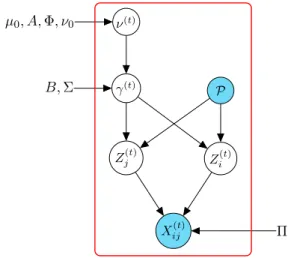
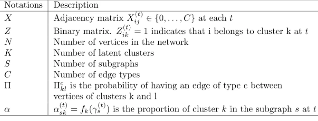
that all parameters in θ depend neither on time nor subgraphs. This model is called thedynamic random subgraph model (dRSM) in the rest of the docu-ment. Figure 3 gives the graphical model for dRSM and Table 1 summarizes the notations used in the model.
At this point, it is possible to see some links and differences between dRSM and dM3SBM (Ho et al., 2011), which is the closest model in the litterature. On
Xij(t) Π Zi(t) Zj(t) P γ(t) B,Σ ν(t) µ0, A,Φ, ν0
Figure 3: Graphical representation of the dRSM model.
the one hand, dRSM and dM3SBM share a common way to model the latent clusters and the temporal dynamic through a state space model. On the other hand, dRSM is able to handle categorical edges, which is a useful feature when working on real-world networks, whereas dM3SBM cannot. In addition, dRSM requires the knowledge of the subgraphs whereas dM3SBM proposes to estimate them. Furthermore, dM3SBM allows the nodes to belong to different clusters. However, allowing to estimate the subgraphs and multi-group belongings may conduce dM3SBM to be a too flexible model and thus to fail in recovering the network structure. Indeed, providing the subgraphs to dRSM allows it to avoid looking for obvious structures such that it can focus on the search of hidden patterns. The comparisons presented in Section 4 seem to confirm this thesis. 2.4. Joint distribution of dRSM
The dRSM model proposed above is defined by the joint distribution:
p(X, Z, γ, ν|θ) =p(X|Z,Π)p(Z|γ)p(γ\K|B, ν,Σ)p(ν|µ0, A,Φ, V0), (2) whereγ\K= (γ (t) s\K)st. Moreover p(X|Z,Π) = T Y t=1 K Y k,l C Y c=0 (Πckl) PN i6=jδ(X (t) ij =c)Z (t) ikZ (t) jl , and p(Z|γ) = T Y t=1 N Y i=1 K Y k=1 fk(γs(t)i ) Zik(t) = T Y t=1 K Y k=1 S Y s=1 fk(γs(t)) PN i=1yisZik(t). (3)
Notations Description
X Adjacency matrixXij(t)∈ {0, . . . , C}at eacht
Z Binary matrix. Zik(t)= 1 indicates that i belongs to cluster k att N Number of vertices in the network
K Number of latent clusters
S Number of subgraphs
C Number of edge types
Π Πc
kl is the probability of having an edge of type c between
vertices of clusters k and l
α α(t)sk =fk(γ
(t)
s ) is the proportion of clusterkin the subgraphsat t
Table 1: Summary of the notations used in the paper.
Note that p(γ\K|B, ν,Σ) = T Y t=1 S Y s=1 N(γs\K(t) ;Bν(t),Σ),
where N(γs\K(t) ;Bν(t),Σ) denotes the multivariate Gaussian distribution, with
mean vectorBν(t)and covariance matrix Σ, evaluated atγs\K(t) . Finally
p(ν|µ0, A,Φ, V0) =p(ν(1)|µ0, V0) T Y t=2 logp(ν(t)|ν(t−1), A,Φ). 3. Estimation
This section focuses on the inference of the model proposed above. A varia-tional EM algorithm is considered and a model selection criterion is derived. 3.1. A variational framework
We aim at maximizing the log-likelihood logp(X|θ) associated with the model. To achieve this maximization, a common approach consists in using an expectation maximization (EM) algorithm (Dempster et al., 1977; Krishnan and McLachlan, 1997). However, such an algorithm cannot be derived here sincep(Z, γ, ν|X, θ) is intractable. Therefore, we propose to use a variational EM-type algorithm (VEM) (Hathaway, 1986) which locally optimizes the model parameters with respect to a lower bound of the log-likelihood. Thus, given a distributionq for the three sets of latent variables (Z, γ, ν), the log-likelihood can be written:
logp(X|θ) =L(q, θ) +KL(q(.)kp(.|X, θ)), (4) whereLis defined as follows:
L(q, θ) =X Z Z γ Z ν q(Z, γ, ν) logp(X, Z, γ, ν|θ) q(Z, γ, ν) dγ dν, (5)
and KL denotes the Kullback-Leibler divergence between the true and approx-imate posterior distributions:
KL(q(.)kp(.|X, θ)) =− X Z Z γ Z ν q(Z, γ, ν) logp(Z, γ, ν|X, θ) q(Z, γ, ν) dγ dν. (6)
Looking for the best approximation of the posterior distributionp(Z, γ, ν|X, θ) in the sense of theKLdivergence becomes equivalent to searching for a distri-butionq(·) that maximizes the lower boundL of the integrated log-likelihood. Unfortunately, because the joint distribution (2) in the lower bound involves the quantity p(Z|γ) which depends on the normalizing constant C(γs(t)), L
has no analytical form and cannot be optimized with respect toq(·). Indeed, C(γs(t)) = log(P
K l=1exp(γ
(t)
sl )) is based on a non linear transformation of the
vector γ(t)s which makes some expectations of the standard VEM algorithm
impossible to derive.
Following the work of Lafferty and Blei (2006) on correlated topic models, we propose a new bound ofL(q, θ) based on a variational lower bound ofp(Z|γ), as in Jordan et al. in Jordan et al. (1999).
Proposition 3.1. (Proof in A) Given any setξof variational parametersξs(t)∈ R∗+, a lower bound of the first lower bound L(q, θ) is given by:
logp(X|θ)>L(q, θ)>L˜(q, θ, ξ), where ˜ L(q, θ, ξ) =X Z Z γ Z ν q(Z, γ, ν) logp(X|Z,Π)h(Z, γ, ξ)p(γ\K|B, ν,Σ)p(ν|µ0, A,Φ, V0) q(Z, γ, ν) dγdν (7) with logh(Z, γ, ξ) = T X t=1 K X k=1 N X i=1 S X s=1 yisZ (t) ik γsk(t)− ξs−1(t) K X l=1 exp(γsl(t))−1+log(ξ(t)s ) .
Note that the variational parameters ξs(t) can be optimized to obtain tight
bounds (see the end of Section 3.2). Moreover, we emphasize that a varia-tional parameterξ(t)s is considered for each subgraphsand each timetfor more
flexibility and to improve the inference procedure. We point out that the qual-ity of the variational approximation we propose cannot be tested analytically since ˜L(q, θ, ξ) and the Kullback-Leibler divergence in (6) are not tractable. Nevertheless, we rely on them for inference purposes. Note that similar approx-imation schemes have been used for instance by Bishop and Svens´en (2003) and Latouche et al. (2014), in the context of model selection.
In order to maximize ˜L(q, θ, ξ), we further assume that q(Z, γ, ν) can be factorized: q(Z, γ, ν) =q(Z)q(γ)q(ν) = T Y t=1 N Y i=1 q(Zi(t))q(γ)q(ν).
Finallyq(γ) is chosen within the family of Gaussian distributions of the form:
q(γ) = T Y t=1 S Y s=1 K Y k=1 N(γ(t)sk; ˆγsk(t),σˆsk2(t)),
to derive analytical expectations in the E step, as in Lafferty and Blei (2006). Since the last component of each vector γ(t)s has to remain equal to zero, to
preserve the bijectivity constraints of the transformation f(·), the terms ˆγsK(t) and ˆσ2(t)
sK are all set to zero to ensure a Dirac mass at zero. All other mean and
variance terms (ˆγsk(t),σˆsk2(t)),∀s, k6=K, t, are parameters to be estimated. 3.2. A VEM algorithm for the dRSM model
In this section, we first assume that the variational terms ξ, which were introduced for approximation purposes, are given. This allows the use of a VEM algorithm (Jordan et al., 1999) to maximize the lower bound ˜L(q, θ, ξ) with respect toq(Z, γ, ν) and the model parameters θ. Such an optimization procedure is iterative and involves a series of successive updates. In the E step, the model parameters are fixed and the lower bound is optimized with respect
toq(Z, γ, ν). Conversely, during the M step, the variational distribution is held
fixed while ˜L(q, θ, ξ) is maximized with respect to θ. In standard VEM algo-rithms, a unique set of latent variables is usually considered. In our case, there are three sets (Z, γ, ν) of latent variables and therefore the E step itself involves iterative updates (as in Latouche et al., 2014, for instance). All distributions
in q(Z, γ, ν) are held fixed, except one, which is optimized. This procedure is
repeated for all distributions in turn.
In the following, we give the update formulae for the E and M steps. The details of the calculations along with the derivation of the lower bound are given in the appendix.
Proposition 3.2. The VEM update step for each distributionq(Zi(t))is given by: q(Zi(t))∼ MZi(t); 1, τi(t)= (τi1(t), . . . , τiK(t)) ∀i, t, where τik(t)∝exp K X l=1 C X c=0 N X i6=j δ(Xij(t)=c)τjl(t)hlog(Πckl) + log(Πclk)i + S X s=1 yis ˆ γsk(t)−ξs−1(t) K X l=1 exp(ˆγsl(t)+σˆ 2(t) sl 2 )−1 + log(ξ (t) s ) ! .
Note thatτik(t) is the approximate posterior probability that nodei belongs to clusterkat timet.
Proposition 3.3. The VEM update step for the distributionq(ν)is given by:
q(ν)∝p(ν(1)|µ0, V0) hYT t=2 p(ν(t)|ν(t−1), A,Φ)ih T Y t=1 N( PS s=1γˆ (t) s S ;Bν (t),Σ S) i .
At this step, we recall that the terms ˆγs(t)are fixed and so is the variablex(t)=
PS
s=1γˆ (t)
s /S. Therefore, it is remarkable to note that the functional form ofq(ν)
corresponds exactly to the form of the posterior distribution associated with a state space model whereν is the set of all latent state variables andx= (x(t))t
the set of observed outputs. Thus, eachx(t)can be written asx(t)=Bν(t)+ ˜v where ˜v∼ N(0,Σ/S) while the variables inν are defined as previously:
ν(t)=Aν(t−1)+ω ν(1)=µ0+u, with ω∼ N(0,Φ) u∼ N(0, V0).
Contrary to the original state space model introduced in Section 2, where both γ and ν were sets of unobserved variables, we obtain here a standard linear dynamic system from which the corresponding parameters, i.e. θ0 =
(µ0, A, B,Φ, V0,Σ/S) can be estimated using Kalman filter and
Rauch-Tung-Striebel (RTS) smoother (Rauch et al., 1965) (details can also be found in Minka, 1998). The expectations ˆν(t) and covariance matrices ˆV(t) of the ran-dom variables ν(t), given all the observed data x, are determined relying on backward forward recursions.
˜ L(q, θ, ξ)simplifies into: ˜ L(q, θ, ξ) = T X t=1 K X k,l C X c=0 N X i6=j δ(Xij(t)=c)τik(t)τjl(t)log(Πckl) + T X t=1 S X s=1 rs(t)γˆ (t) sk −Nsξ−1(t)s K X l=1 exp(ˆγsl(t)+σˆ 2(t) sl 2 ) +Ns−Nslog(ξ (t) s ) + T X t=1 S X s=1 logN(ˆγs(t), Bνˆs(t),Σ)−1 2tr(Σ −1B|Vˆ(t)B) −1 2tr(Σ −1σˆ(t)2 s ) − T X t=1 S X s=1 K−1 X k=1 −log(2π)12ˆσ(t) sk +T KS 2 − T X t=1 logN(x(t);Bνˆ(t),Σ S) + 1 2tr(Σ −1SB|Vˆ(t)B) − N X i=1 T X t=1 K X k=1 τik(t)log(τik(t)) + logp(x|θ0)
where r(t)s = PNi=1τik(t)yis, Ns is a number of nodes in the subgraph s, and
logp(x|θ0)is the log likelihood of the linear dynamic system associated with the variational distributionq(ν) (see Proposition 3.3)
The maximization of this bound allows to obtain the updating formula for the tensor matrix Π: ˆ Πckl = PT t=1 PN i6=jδ(X (t) ij =c)τ (t) ik τ (t) jl PT t=1 PC c=0 PN i6=jδ(X (t) ij =c)τ (t) ikτ (t) jl ,∀k, l, c.
For the parameters ˆγsk(t) and ˆσsk2(t), we do not obtain analytical expressions, and therefore we rely on a quasi-Newton algorithm for the optimization task. 3.3. Optimization ofξ
So far, we have seen that a VEM algorithm could be implemented from approximations depending on the variational parametersξ(t)s . However, we have
not addressed yet how these parameters could be estimated from the data. We follow the work of Svens´en and Bishop (2004) on Bayesian hierarchical mixture of experts. Thus, the lower bound ˜L(q, θ, ξ) is optimized with respect to the variational terms ξs(t) to obtain the tightest bound ˜L(q, θ, ξ) of L(q, θ). This
leads to new estimates ˆξs(t) ofξs(t):
ˆ ξ(t)s = K X l=1 exp(ˆγsl(t)+ ˆσ2sl(t)),∀s, t.
This procedure gives rise to a three step optimization scheme. Given all ξ = (ξs(t))st, the VEM algorithm described previously is used to maximize the lower
bound with respect toq(Z, γ, ν) and θ. These terms are then held fixed and a new estimate ofξ is computed. The three steps are repeated until convergence of the lower bound.
3.4. Model selection: choice of the numberK of latent groups
Using the VEM algorithm proposed in the previous paragraphs, the estima-tion of the model parameters and of the group memberships is fully automatic for a given value ofK. Since we consider here a model-based approach, two dRSM models with different values ofKcan be considered as two different models. The problem of choosingKcan therefore be viewed as a model selection problem. It can be tackled in a model-based context using model selection criteria, such as the Akaike information criterion (AIC) (Akaike, 1974) or the Bayesian informa-tion criterion (BIC) (Schwarz, 1978). Due to its popularity and its asymptotic properties (Leroux, 1992), we use BIC in the numerical experiments presented in the following sections. BIC relies on an asymptotic approximation of the marginal log-likelihood, also called integrated log-likelihood, and is defined in the specific context of the dRSM modelMby:
BIC(M) = logp(X|θ)ˆ −η(M)
2 log(T N(N−1)),
whereη(M) is the number of free model parameters depending onK, for the identifiability constraints considered. Unfortunately, the log-likelihood logp(X|θ) =ˆ logP
Zp(X, Z|θˆ
is not tractable here because it involves marginalizing over all latent vectorsZi(t) in Z. Therefore, we propose to replace the log-likelihood with its variational approximation ˜L(q, θ, ξ). Thus, the VEM algorithm is run for various values ofK. For eachK, the algorithm iterates until convergence of the lower bound. ˆK is then chosen such that the (approximate) BIC criterion is maximized.
4. Numerical experiments and comparisons
This section aims at proving on synthetic data the validity of the inference algorithm presented in section 3. An introductory example is first considered to highlight the main features of the proposed approach. Model selection is then considered to validate the criterion choice. Extensive comparisons with state-of-the-art methods conclude this section.
4.1. Experimental setup
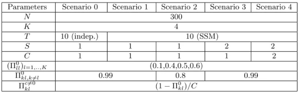
In order to validate our approach, we use in this section artificial data gen-erated according to a common experimental setup. To simplify the character-ization and facilitate the reproducibility of the experiments, we designed five different scenarios. The generation setup for each scenario is summarized in
Parameters Scenario 0 Scenario 1 Scenario 2 Scenario 3 Scenario 4 N 300 K 4 T 10 (indep.) 10 (SSM) S 1 1 1 2 2 C 1 1 1 1 2 (Π0 ll)l=1,..,K (0.1,0.4,0.5,0.6) Π0 kl,k6=l 0.99 0.8 0.99 Πckl6=0 (1−Π0 kl)/C
Table 2: Parameter values for the five types of graphs used in the experiments. In scenario 0, the networks are drawn without an explicit temporal dependance whereas, in the other scenarios, the temporal dependance is generated through a state space model (SSM).
Table 2. Data from scenario 0 are drawn using SBM at each timetand without an explicit temporal dependence. The data sets for all other scenarios (scenar-ios 1 to 4) are drawn according to the dRSM model. Therefore, the temporal dependence is generated through a state space model. All generated networks are made of N = 300 nodes, distributed into K = 4 latent groups and have T = 10 time points. Depending on the scenario, the networks have S= 1 or 2 subgraphs, with binary (C= 1) or categorical (C= 2) edges. WhenS >1, the nodes are randomly assigned uniformly to the subgraphs. Notice that scenario 2 has a parameter Π0
kl,k6=lequal to 0.8 which leads to less heterogeneous latent
groups.
The model parameters used for the simulation are as follows. For the sim-ulation ofγ, it is assumed that the matrices A, B andV0 are set toIK−1, and
that Σ = 0.1×K×IK−1 and Φ = 0.01×IK−1. Finally, the tensor matrix Π,
which defines the connection probabilities between clusters for theC different types, is set up such that, within the clusters, the probability 1−Π0
llof having
an edge of any type is larger than the corresponding connection probabilities be-tween clusters 1−Π0
kl,k6=l(see Table 2). Notice that such a choice of parameters
induces networks made of communities. Then, in case of a connection between two nodes, the edge type is sampled uniformly,i.e. Πc6=0kl = (1−Π0
kl)/C, ∀k, l.
4.2. An introductory example
We first focus on an introductory example to illustrate the global behavior of the proposed methodology. To this end, we simulated a single network according to scenario 2 for facilitating the understanding of the results. We remind that in this setup the number K of latent groups is fixed to 4 and that C = 1. Therefore, the network is binary and Π1
kl indicates the occurrence probability
of an edge. We ran the VEM algorithm on it for a numberK of groups ranging from 3 to 6. We selected afterward the most appropriate number of groups using the BIC criterion.
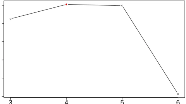
Figure 4 shows the BIC values associated to the results provided by our VEM algorithm for the different values ofK. One can observe that the criterion picks at K = 4, which is the actual simulated value for K. Figure 5 presents the
● ● ● ● −300000 −260000 −220000 Choice of K K BIC 3 4 5 6 ●
Figure 4: Choice ofKby model selection with BIC for a simulated network. The actual value
forKis 4.
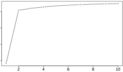
evolution of the bound ˜L for this specific value ofK along the 10 iterations of the VEM algorithm. A clear plateau of the bound is visible on the figure, which indicates the convergence of the algorithm.
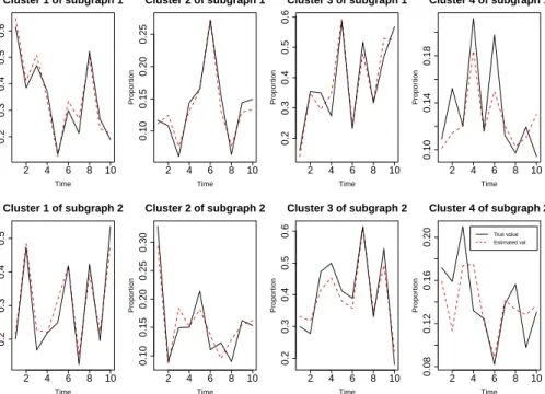
To quickly assess the estimation quality, Table 3 allows to compare the actual (left panel) and estimated (right panel) values of the terms Π1kl in the tensor matrix Π, which define the connection probabilities between the latent clusters. On this single example, the estimated values Π1kl turn out to be extremely close to the true ones. Similarly, Figure 6 compares the actual (dashed red lines) and estimated (solid black lines) values of the group proportionsαfor the simulated example. Once again, the estimation ofαappears to be very close to the true proportions.
4.3. Choice of K
We now focus on the evaluation of the criterion we proposed to select the number K of latent groups. Since our approach aims at searching the unob-served clustering partition of the nodes, we chose here to evaluate the combina-tion of our VEM algorithm with the BIC criterion by comparing the resulting partition with the actual one (the simulated partition). In the clustering com-munity, the adjusted Rand index (ARI) (Rand, 1971) serves as a widely accepted criterion for the difficult task of clustering evaluation. The ARI looks at all pairs of nodes and check wether they are classified in the same group or not in both partitions. As a result, an ARI value close to 1 means that the partitions are similar and, in our case, that the VEM algorithm succeeds in recovering the simulated partition.
To validate the combination of our VEM algorithm with the BIC criterion, the analysis was repeated for 50 different data sets, generated according to scenario 2, for a numberK of latent groups ranging from 3 to 6. This allows us
● ● ● ● ● ● ● ● ● ● 2 4 6 8 10 −197970 −197950
Evolution of the bound for K=4
Iterations
V
alue of the bound
Figure 5: Evolution of the bound ˜LforK= 4.
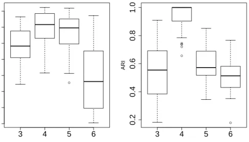
to both verify the consistency of the BIC criterion and to study the clustering ability of our approach. Figure 7 shows the repartition of the criterion values (left panel) as well as the associated ARI values (right panel). These results first confirm that BIC is a valid criterion for selecting the number of groups in this context. Indeed, the valueK = 4 is the one which is the most frequently associated with the highest value of BIC. We remind thatK = 4 is the actual number of latent groups. One can also observe that the partition resulting from our VEM algorithm is associated, for this value ofK, to an ARI value extremely close to 1 which denotes a good matching with the actual partition of the data. 4.4. Comparison with the other stochastic models
Our third set of experiments now aims at comparing the performance of our approach to that of state-of-the-art methods. We are here interested in the comparison of dRSM with the following methods: SBM (Nowicki and Snijders, 2001), RSM (Jernite et al., 2014) and dM3SBM (Ho et al., 2011). Once again, the evaluation of the results is done using the ARI criterion. In order to fit a SBM on a dynamic network, we ran the mixer package (Ambroise et al., 2010) for the R software at each timet and the ARI is then computed on the concatenation of all group labels. However, let us notice that SBM was not able to handle networks with categorical edges (scenario 3). For RSM, we used the
Rambopackage (Bouveyron et al., 2013) for R, on an aggregated version of the
whole network. Conversely to SBM, RSM is only able to deal with categorical networks and, consequently, it works only in scenario 4. Finally, we used the Matlab toolboxdM3SBM, kindly provided by the authors, to fit the dM3SBM on the dynamic networks. However, dM3SBM is also not able to handle networks with categorical edges (scenario 4).
Cluster 1 2 3 4 1 0.90 0.01 0.01 0.01 2 0.01 0.60 0.01 0.01 3 0.01 0.01 0.50 0.01 4 0.01 0.01 0.01 0.40 Cluster 1 2 3 4 1 0.89 0.01 0.01 0.01 2 0.01 0.59 0.01 0.01 3 0.01 0.01 0.48 0.01 4 0.01 0.01 0.01 0.39
Actual values Estimated values
Table 3: Actual (left) and estimated (right) values for the terms Π1
klof the tensor matrix Π.
See text for details.
2 4 6 8 10 0.2 0.3 0.4 0.5 0.6 Cluster 1 of subgraph 1 Time Propor tion 2 4 6 8 10 0.10 0.15 0.20 0.25 Cluster 2 of subgraph 1 Time Propor tion 2 4 6 8 10 0.2 0.3 0.4 0.5 0.6 Cluster 3 of subgraph 1 Time Propor tion 2 4 6 8 10 0.10 0.14 0.18 Cluster 4 of subgraph 1 Time Propor tion 2 4 6 8 10 0.2 0.3 0.4 0.5 Cluster 1 of subgraph 2 Time Propor tion 2 4 6 8 10 0.10 0.15 0.20 0.25 0.30 Cluster 2 of subgraph 2 Time Propor tion 2 4 6 8 10 0.2 0.3 0.4 0.5 0.6 Cluster 3 of subgraph 2 Time Propor tion 2 4 6 8 10 0.08 0.12 0.16 0.20 Cluster 4 of subgraph 2 Time Propor tion True value Estimated val.
Figure 6: Actual (dashed red lines) and estimated (solid black lines) values of the group
● 3 4 5 6 −320000 −260000 −200000
Choice of K
K BIC ● ● ● ● ● ● 3 4 5 6 0.2 0.4 0.6 0.8 1.0Clustering accuracy
K ARIFigure 7:Criterion and ARI values over 50 networks generated.
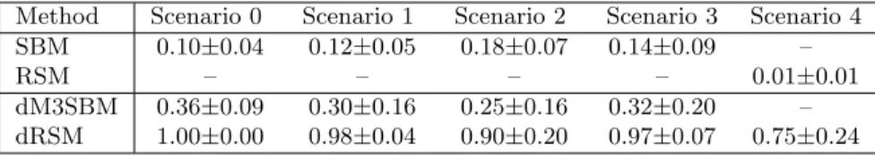
In order to consider a wide type of networks, we compare here the methods over the five simulation scenarios. We remind that Table 2 summarizes the main features of each scenario. This comparison has been conducted in two different situations: with and without the knowledge of the actual number of clusters. Table 4 presents the clustering results for the four studied methods in the case where the actual number K = 4 of groups has been provided to each method. Conversely, Table 5 presents the clustering results when the methods have to look for the value ofK. Reported values are averaged ARI values (with standard deviations) on 20 networks for each scenario. The average selected numberK of latent groups is also provided for Table 5.
First, for scenarios 0, 1 and 2, which consider dynamic networks with binary edges (C = 1) and with only one subgraph (S = 1), one can see on Tables 4 and 5 that SBM is, as expected, not able to handle the network dynamic. In-deed, SBM obtains a low ARI value in all situations, even though it correctly estimates the number of clusters (Table 5). Conversely, the two dynamic meth-ods (dM3SBM and dRSM) turn out to be able to recover the clustering structure of the dynamic networks. One can however notice that dRSM significantly out-performs dM3SBM in this situation. Notice also the accurate estimation of the numberK of clusters made by dRSM (Table 5).
In scenario 3, the simulated dynamic networks are now made of two sub-graphs (S= 2), still with binary edges (C= 1). Naturally, SBM does not per-form well in this situation too. The dM3SBM provides clustering results similar to the ones of previous scenarios: it globally succeeds in recovering the dy-namic but fails in recognizing the clustering pattern. On the other hand, dRSM provides again accurate clustering results associated with good estimations of
Method Scenario 0 Scenario 1 Scenario 2 Scenario 3 Scenario 4
SBM 0.10±0.04 0.12±0.05 0.18±0.07 0.14±0.09 –
RSM – – – – 0.01±0.01
dM3SBM 0.36±0.09 0.30±0.16 0.25±0.16 0.32±0.20 –
dRSM 1.00±0.00 0.98±0.04 0.90±0.20 0.97±0.07 0.75±0.24
Table 4: Clustering results for the four studied methods on networks simulated according to
the five scenarios. The actual numberK = 4 of groups has been provided to each method
here. Average ARI values are reported (with standard deviations) and results are averaged on 20 networks for each scenario.
K, meaning that it succeeds in identifying both the dynamic and clustering patterns.
Finally, scenario 4 considers the case of dynamic networks with two sub-graphs (S = 2) and categorical edges (C = 2). Only RSM and dRSM are able to deal with this kind of networks. Similarly to SBM in previous scenarios, RSM does not succeed in recovering the dynamic and provides very unsatis-factory clustering results. Conversely, dRSM gives very good clustering results regarding the difficulty of the situation. It is worth noticing the sharp estima-tion made by dRSM of the numberK of group in this case too. This confirms the efficiency of both our inference algorithm and our model selection criterion. We also used scenario 4 to highlight that providing the methodology with the right subgraph structure helps in clustering the vertices. Thus, with the knowledge of the actual number of clusters, we ran dRSM with the wrong sub-graph structure (S = 1), and we obtained an average ARI of 0.54±0.2. This result is to be compared to the ARI performances for scenario 4, as presented in Table 4.
5. Maritime network
This section presents an application of the proposed methodology for the analysis of a network of maritime flows in which a temporal dynamic is present. The dynamic network was provided by Dr. C´esar Ducruet, from the G´ eographie-Cit´es laboratory, who is interested in studying the evolution of maritime flows over time. The data was extracted from the well-known Lloyd’s list which has recorded almost all ship movements worldwide since 1890.
5.1. Data and study protocol
Data was obtained from the printed Lloyds voyage record published every October between 1890 until 2008. The list details, for each merchant vessel, its successive movements from one port to another. From the raw database of vessel flows, we extracted a dynamic network with 17 time points. The first observation is October 1890 and the network ends in October 2008. Table 6 provides the correspondence between the 17 time points and the actual dates.
At each time point, the adjacency matrix between ports was constructed as follows. First, for every pair of ports, we calculated the total number of
Scenario 0 Scenario 1 Scen ario 2 Scenario 3 Scenario 4 Metho d ARI K ARI K ARI K ARI K ARI K SBM 0.01 ± 0.04 4.00 ± 0.00 0.18 ± 0.13 3.94 ± 0.71 0.21 ± 0.11 3.97 ± 0.46 0.13 ± 0.05 4.16 ± 0.79 – – RSM – – – – – – – – 0.01 ± 0.01 2.00 ± 0.00 dM3SBM 0.01 ± 0.01 5.55 ± 1.39 0.35 ± 0.21 5.95 ± 1.15 0.30 ± 0.21 4.35 ± 1.63 0.32 ± 0.19 5.15 ± 1.17 – – dRSM 1.00 ± 0.00 4.00 ± 0.00 0.87 ± 0.17 4.01 ± 0.65 0.89 ± 0.21 4.10 ± 0.30 0.85 ± 0.22 4.10 ± 0.45 0.68 ± 0.30 4.05 ± 0.51 T able 5: Cl u ste ri ng results for the four studied metho ds on net w o rks sim ulated according to the fiv e scenarios. Av erage ARI v a lu e s are rep orted (with standard deviations) as w ell as the selected n um b er K of laten t groups. Results are a v eraged on 20 net w orks for eac h scenario.
Time point Date
t1 October 1890
t2. . . t4 October 1925 to October 1940, every five years
t5 October 1946
t6 October 1951
t7 October 1960
t8. . . t16 October 1965 to October 2000, every five years
t17 October 2008
Table 6: The time points considered in the maritime network.
ship movements between those ports. Then, we set the associated entry in the adjacency matrix to 1 if the number of ship movements between the two ports is greater or equal to 1, and to 0 otherwise. The original network contained 4472 ports worldwide. We however had to reduce the network size to only 286 ports since most of the ports were not active throughout the whole period of the study.
We finally applied dRSM to a maritime network which describes the naviga-tion of ships among 286 ports in the world at 17 time points. Let us highlight that the study period includes many major historical or economical events (the two world wars, the oil crisis, the economic crisis in Europe, ...), which could directly affect the navigation movements at a global scale and could also change the port behaviors.
The partition of the network into subgraphs is here provided by the port memberships to the four main maritime basins: Asia – Pacific, Europe – At-lantic, Mediterranean – Black Seas, and Middle East – Indian Ocean. Figure 8 presents this partition of the ports where the colors indicates the different sub-graphs.
To summarize, the network is a undirected and binary network without self loops, i.e. C = 1 and Xijt = 1 if the port i and the portj exchange at least one ship during the period t, 0 otherwise, with t ∈ {1, . . . ,17} and S = 4. Figure 9 shows the adjacency matrix, in 1890 and in 2008, between the 286 ports organized by subgraph.
5.2. Results
We used the variational EM algorithm introduced in the previous section in order to find the latent groups that may be hidden in the data. The choice of the number of groups is made by applying the VEM algorithm forK = 3, ...,8 and by then computing the associated BIC values. The retained value forK is the one associated with the highest BIC value. To ensure a good accuracy of the results, the VEM algorithm was run 5 times for each value ofK. Figure 10 shows the evolution of the BIC criterion according toK. One can observe that BIC peaks atK= 7, meaning that 7 latent groups seem to organize the network. We therefore chose this specific value forKand retained the best run forK= 7 over the five runs as the final clustering result.
Figure 8: The given partition of the 286 nodes (ports) into 4 subgraphs.
Network in 1890 Network in 2008
Figure 9: Adjacency matrix of the maritime network organized by subgraph (basin) in 1890 (left) and 2008 (right).
● 3 4 5 6 7 8 −288000 −284000 −280000 −276000 Choice of K K BIC
Figure 10: BIC values according to the numberKof groups for the maritime network.
On the one hand, it is of main interest to look at the estimated tensor matrix Π in order to understand and characterize the found latent groups. Indeed, the tensor matrix Π describes the connection probabilities between the groups and allows to figure out the different connection patterns. Since the network considered here is binary, it is enough to look at the terms Π1
kl since Π 0 kl +
Π1
kl = 1, for all k, l. Figure 11 presents those estimated values. From the
figure, clusters 6 and 7 appear to be groups of hubs for which the connection probabilities are large within and between clusters.
On the other hand, the estimated group proportions over time should allow to understand the dynamic of the network. Figure 12 presents the evolution of those proportions over time for each subgraph. One can first observe that the proportion of cluster 6 is low and rather stable over time. This confirms that cluster 6 is a group of a limited number of hubs with a high connectivity and probably a high level of traffic. Cluster 6 includes ports such as Anvers, Rotterdam or Singapore. It is also interesting to see that, in subgraph 2 (Europe – Atlantic), the number of hubs increased until 1930, was then perturbed during the second world war and finally decreased from 1951. Conversely, in subgraph 1 (Asia – Pacific), the proportion of hubs was low until 1975 and then significantly increased. From a global point of view, one can also observe a clear and recent reorganization of the network in which hubs tend to be less numerous worldwide (and probably bigger).
Regarding cluster 7, one can see on Figure 12 that its proportions in the subgraphs are higher than those of cluster 6. The ports of cluster 7 can be qualified as hubs of second class which are subordinated to the main hubs of cluster 6. Most of them are marked by a colonial logic, such as Marseille,
0.2% 1.3% 0.4% 0.6% 1.2% 9.3% 2.8% 1.3% 11.8% 2% 6% 6% 51.9% 23.6% 0.4% 2% 3.3% 0.3% 9.4% 37% 11.6% 0.6% 6% 0.3% 3.3% 1.2% 25.4% 9% 1.2% 6% 9.4% 1.2% 23.7% 68.9% 30.5% 9.3% 51.9% 37% 25.4% 68.9% 86.6% 83.6% 2.8% 23.6% 11.6% 9% 30.5% 83.6% 50.6% Cluster 1 Cluster 2 Cluster 3 Cluster 4 Cluster 5 Cluster 6 Cluster 7
Cluster 1 Cluster 2 Cluster 3 Cluster 4 Cluster 5 Cluster 6 Cluster 7 Connection probabilities between clusters
0.0 0.2 0.4 Subgraph 1 (Asia − P acific) Time Group proportions 1890 1930 1940 1951 1965 1975 1985 1995 2008 0.0 0.1 0.2 0.3 0.4 Subgraph 2 (Eur ope − Atlantic) Time Group proportions 1890 1930 1940 1951 1965 1975 1985 1995 2008 0.0 0.2 0.4
Subgraph 3 (Medit. − Blac
k Sea) Time Group proportions 1890 1930 1940 1951 1965 1975 1985 1995 2008 0.0 0.1 0.2 0.3 0.4 Subgraph 4 (Mid
dle East − India)
Time Group proportions 1890 1930 1940 1951 1965 1975 1985 1995 2008 G1 G2 G3 G4 G5 G6 G7 Figure 12: Ev olution of the prop ortions of the K = 7 laten t clusters.
Kolkata or Cape Town. The evolution of this cluster until the recent period shows a persisting link North-South (e.g. Le Havre - Casablanca) or East-West (e.g. Spain - Brazil - Canaries).
The cluster 5 is mainly made of ports from the Asia – Pacific and Middle East – India basins except during major crises, such as World War II and the oil crisis. During those crises, the cluster mainly contains European ports. The rapid modification of this cluster appears clearly on Figure 12 around 1946, 1980 and 2008. This cluster can be interpreted as made of active ports from the developing world which move to cluster 2 during the crises. This may highlight the disintegration of long distance links during such crises. Conversely, cluster 2 turns out to be mostly made, except during crises, of European ports of average size, mainly on the atlantic coast. Those ports are rather a reflection of a past glory and most of them have declined over the century. This may due to a failed industrialization or a significant distance to the major trade routes.
Finally, clusters 3 and 4 are made of very small ports with low activity. Those ports are usually not connected together and communicate with the rest of the network only through ports of clusters 2 and 5. The connection with clusters 2 and 5 explains the brutal changes in the proportions of clusters 3 and 4 that one can also observe.
6. Conclusion
This work has considered the problem of analyzing dynamic networks with categorical edges and for which a subgraph partition is known. This kind of networks is frequent in a wide range of scientific fields, such as Geography in particular. For this purpose, we proposed an extension of the RSM model to the dynamic setting. The new model, called dRSM, uses a state space model to model the evolution of the latent group proportions over time. A variational ex-pectation maximization (VEM) algorithm is proposed to perform inference. We have shown in particular that the variational approximations lead to a new state space model from which the parameters can be estimated using the standard Kalman filter and the Rauch-Tung-Striebel (RTS) smoother. Model selection is also considered through an approximate BIC criterion.
Numerical experiments have highlighted the main features of the dRSM model and have demonstrated the efficiency of both the VEM algorithm and the model selection criterion. A numerical comparison has also shown that existing methods, dynamic or not, are less flexible and efficient than dRSM when applied to dynamic networks. Finally, dRSM has been applied to a dynamic maritime flow network, build from the famous Lloyd’s list, and has allowed to characterize interesting dynamic phenomena.
Acknowledgments
The authors would like to greatly thank C´esar Ducruet, from the G´ eographie-Cit´es laboratory, Paris, France, for providing the maritime network and for his
painstaking analysis of the results. The data were collected in the context of the ERC Grant N.313847 ”World Seastems” (http://www.world-seastems.cnrs.fr). The authors would like also to thank Catherine Matias and St´ephane Robin for their useful remarks and comments on this work.
A. Construction of a tractable lower bound
We rely on a bound introduced in Jordan et al. (1999). Such a general bound can easily been derived by noticing that C(·) is a concave function of
PK
l=1exp(γ (t)
sil) and therefore a first order Taylor expansion of the normalizing constant, at anyξs(t)∈R∗+, will lead to the inequality:
log( K X l=1 exp(γsl(t)))≤ξ−1(t)s ( K X l=1 exp(γsl(t)))−1 + log(ξs(t)). (8)
The bounds (8) on the C(γs(t)) terms induce a lower bound on the quantity
logp(Z|γ): logp(Z|γ) = T X t=1 K X k=1 N X i=1 Zik(t)log(fk(γ(t)si )) = T X t=1 K X k=1 N X i=1 S X s=1 yisZ (t) ik γsk(t)−log( K X l=1 exp(γsl(t))) ≥ logh(Z, γ, ξ),
where ξ denotes the set of all variational parameters (ξs(t))st and the function
h(·,·,·) is such that: logh(Z, γ, ξ) = T X t=1 K X k=1 N X i=1 S X s=1 yisZ (t) ik γsk(t)− ξs−1(t) K X l=1 exp(γsl(t))−1+log(ξ(t)s ) .
Replacing logp(Z|γ) by logh(Z, γ, ξ) in L(q, θ), leads to a new lower bound ˜
L(q, θ, ξ) for logp(X|θ) which satisfies:
logp(X|θ)>L(q, θ)>L˜(q, θ, ξ), where ˜ L(q, θ, ξ) =X Z Z γ Z ν q(Z, γ, ν) logp(X|Z,Π)h(Z, γ, ξ)p(γ|B, ν,Σ)p(ν|µ0, A,Φ, V0) q(Z, γ, ν) dγdν.
B. E-step of the VEM algorithm Distributionq(Z)
The VEM update step for each of the distributions q(Zi) in q(Z) is given
by:
logq(Zi) = Eγ,ν,Z\i[logp(X|Z,Π) + logh(Z, γ, ξ)] + const
= T X t=1 K X k=1 Zik(t) K X l=1 C X c=0 N X i6=j δ(Xij(t)=c)τjl(t)hlog(Πckl) + log(Πclk)i + T X t=1 K X k=1 S X s=1 yisEγ h Zik(t)logh(Z(t), γ(t), ξ(t))i+ const. = T X t=1 K X k=1 Zik(t) K X l=1 C X c=0 N X i6=j δ(Xij(t)=c)τjl(t)hlog(Πckl) + log(Πclk)i + T X t=1 K X k=1 S X s=1 yisEγ h γsk(t)−(ξ−1(t)s K X l=1
exp(γsk(t))−1 + log(ξs(t)))i+ const.
= T X t=1 K X k=1 Zik(t) K X l=1 C X c=0 N X i6=j δ(Xij(t)=c)τjl(t)hlog(Πckl) + log(Πclk) i + T X t=1 K X k=1 S X s=1 Zik(t)yis γˆ (t) sk − h ξs−1(t) K X l=1 E(exp(γsl(t)))−1 + log(ξs(t))i ! + const. = T X t=1 K X k=1 Zik(t) K X l=1 C X c=0 N X i6=j δ(Xij(t)=c)τjl(t)hlog(Πckl) + log(Πclk)i + S X s=1 yis ˆ γ(t)sk −ξ−1(t)s K X l=1 exp(ˆγsl(t)+σˆ 2(t) sl 2 )−1 + log(ξ (t) s ) ! + const,
where all terms that do not depend onZihave been put into the constant terms
const. Moreover sinceγ(t)sk ∼ N(ˆγsk(t),σˆ2(t)
sk ) we have used: E[exp(γsk(t))] = exp(ˆγ (t) sk + ˆ σ2(t) sk 2 ).
We then recognize the functional form of a multinomial distribution: q(Zi(t))∼ M(Zi(t); 1, τi(t)), ∀i, t.
Distributionq(ν):
The VEM update step for the distributionq(ν) is given by: logq(ν) = EZ,γ logp(γ|ν,Σ, B) + logp(ν|µ0, V0, A,Φ) + const = T X t=1 S X s=1 Eγ logN(γs(t);Bν (t),Σ) + logp(ν(1)|µ0, V0) + T X t=2 logp(ν(t)|ν(t−1), A,Φ) + const = T X t=1 S X s=1 Eγ − 1 2(γ (t) s )|Σ −1(γ(t) s ) + (γ (t) s )|Σ −1Bν(t)−1 2(ν (t))|B|Σ−1Bν(t) + logp(ν(1)|µ0, V0) + T X t=2 logp(ν(t)|ν(t−1), A,Φ) + const. = T X t=1 XS s=1 ˆ γs(t)Σ−1Bν(t)−1 2(ν (t))|B|(SΣ−1)Bν(t) + logp(ν(1)|µ0, V0) + T X t=2 logp(ν(t)|ν(t−1), A,Φ) + const,
where all terms that do not depend onνhave been put into the constant terms const. We recognize the functional form of the posterior distribution of a linear dynamic system: logq(ν) = T X t=1 logN( PS s=1γˆ (t) s S ;Bν (t),Σ S) + logp(ν(1)|µ0, V0) + T X t=2 logp(ν(t)|ν(t−1), A,Φ) + const.
C. Derivation of the lower bound In the following, we denote x(t) =
PS
s=1γˆ (t) s
S an observed variable. The lower bound is given by:
˜ L(q, θ, ξ) = X Z Z γ Z ν q(Z, γ, ν) logp(X|Z,Π)h(Z, γ, ξ)p(γ|ν,Σ)p(ν|µ0, A,Φ, V0) q(Z, γ, ν) dνdγ = EZ,γ,ν[log p(X|Z,Π)h(Z, γ, ξ)p(γ|ν,Σ, B)p(ν|µ0, A,Φ, V0) q(γ)q(ν)QN i=1q(Zi) ]
= EZ(logp(X|Z,Π)) +EZ,γ(logh(Z, γ, ξ)) +Eγ,ν(logp(γ|ν,Σ, B))
+ Eν(logp(ν|µ0, A,Φ, V0))−Eγ(logq(γ))−Eν(logq(ν))−EZ(log(
N
Y
i=1
q(Zi))).
Note that (see Proposition 3.3),
q(ν)∝p(ν(1)|µ0, V0) hYT t=2 p(ν(t)|ν(t−1), A,Φ)ih T Y t=1 N( PS s=1γˆ (t) s S ;Bν (t),Σ S) i .
As pointed out in this proposition, this corresponds to the form of the posterior distribution associated with a state space model with parameter θ0 and with observed outputs x = (x(t))t. If we denote p(x|θ
0
) the likelihood associated with this model, and the joint likelihoodp(x, ν|θ0), we have
q(ν) =p(x, ν|θ 0 ) p(x|θ0 ) . Therefore
Eν(logq(ν)) =Eν(logp(ν|µ0, A,Φ, V0))+Eν(logp(
PS s=1ˆγ (t) s S |ν (t),Σ S, B))−logp(x|θ 0 ). This leads to,
Eν(logp(ν|µ0, A,Φ, V0))−Eν(logq(ν)) =−Eν(logp(
PS s=1γˆ (t) s S |ν (t),Σ S, B))+logp(x|θ 0 ),
and ˜L(q, θ, ξ) can be written as follows: ˜ L(q, θ, ξ) = X Z Z γ Z ν q(Z, γ, ν) logp(X|Z,Π)h(Z, γ, ξ)p(γ|ν,Σ)p(ν|µ0, A,Φ, V0) q(Z, γ, ν) = EZ,γ,ν[log p(X|Z,Π)h(Z, γ, ξ)p(γ|ν,Σ, B)p(ν|µ0, A,Φ, V0) q(γ)q(ν)QN i=1q(Zi) ]
= EZ(logp(X|Z,Π)) +EZ,γ(logh(Z, γ, ξ)) +Eγ,ν(logp(γ|ν,Σ, B))
− Eγ(logq(γ))−Eν(logp( PS s=1ˆγ (t) s S |ν (t),Σ S, B))−EZ(log( N Y i=1 q(Zi))) + logp(x|θ0).
We explicit below each of the terms of the bound ˜L(q, θ). 1. EZ(logp(X|Z,Π)): EZ(logp(X|Z,Π)) = T X t=1 K X k,l C X c=0 N X i6=j Ez(δ(X (t) ij =c)Z (t) ikZ (t) jl log(Π c kl) = T X t=1 K X k,l C X c=0 N X i6=j δ(Xij(t)=c)τik(t)τjl(t)log(Πckl) 2. EZ,γ(logh(Z, γ, ξ)): EZ,γ(logh(Z, γ, ξ)) = EZ,γ hXT t=1 K X k=1 N X i=1 S X s=1 yisZ (t) ik γ(t)sk − ξ−1(t)s X l exp(γsk(t)) − 1 + log(ξs(t))i = T X t=1 K X k=1 N X i=1 S X s=1 yis τik(t)ˆγ(t)sk −τik(t)ξ−1(t)s K X l=1 exp(ˆγsl(t)+ˆσ 2(t) sl 2 ) + τik(t)−τik(t)log(ξ(t)s ) = T X t=1 S X s=1 rs(t)γˆsk(t)−Nsξs−1(t) K X l=1 exp(ˆγsl(t)+σˆ 2(t) sl 2 ) +Ns−Nslog(ξ (t) s )
where denoter(t)s is a quantityP N i=1τ
(t) ikyis.
3. Eγ,ν(logp(γ|ν,Σ, B)): Eγ,ν(logp(γ|ν,Σ, B)) = Eγ,ν log T Y t=1 S Y s=1 N(γs(t);Bνs(t),Σ) = T X t=1 S X s=1 logN(ˆγs(t), Bˆνs(t),Σ)−1 2tr(Σ −1BTVˆ(t)B)−1 2tr(Σ −1σˆ(t)2 s ) 4. Eγ(logq(γ)): Eγ(logq(γ)) = Eγ YT t=1 S Y s=1 K Y k=1 N(γ(t)sk; ˆγsk(t),ˆσsk2(t)) = T X t=1 S X s=1 K X k=1 −log(2π)12ˆσ(t) sk −T KS 2 . 5. Eν(logp( PS s=1ˆγ (t) s S |ν (t),Σ S, B)) : Eν(logp( PS s=1ˆγ (t) s S |ν (t),Σ S, B)) = T X t=1 logN(x(t);Bνˆ(t),Σ/S)−1 2tr(Σ −1SBTVˆ(t)B). 6. EZ(log(Q T i=1q(Zi))): EZ(log( T Y i=1 q(Zi))) = N X i=1 EZ(logq(Zi)) = N X i=1 EZ( T X t=1 K X k=1 Zik(t)log(τik)) = N X i=1 T X t=1 K X k=1 τik(t)log(τik(t)).