Variable selection and structural discovery in joint models of longitudinal and survival data

(1)

VARIABLE SELECTION AND STRUCTURAL DISCOVERY IN

JOINT MODELS OF LONGITUDINAL AND SURVIVAL DATA

Zangdong He

Submitted to the faculty of the University Graduate School in partial fulfillment of the requirements

for the degree Doctor of Philosophy in the Department of Biostatistics,

Indiana University December, 2014

(2)

Accepted by the Graduate Faculty, Indiana University, in partial fulfillment of the requirements for the degree of Doctor of Philosophy.

Doctoral Committee

November 04, 2014

Wanzhu Tu, Ph.D., Co-chair

Zhangsheng Yu, Ph.D., Co-chair

Hai Liu, Ph.D.

(3)

c

2014 Zangdong He

(4)

DEDICATION

(5)

ACKNOWLEDGMENTS

I would like to express sincere gratitude to my advisors Dr. Wanzhu Tu and Dr. Zhangsheng Yu for their constant guidance, encouragement and support in my Ph.D. study. I really appreciate the opportunity that they lead me to grow in this wonderful research area. Their guidance has not only trained my knowledge and expertise, but also cultivated me with open-mindedness, ability of critical thinking, and skills of effective communication which are essential for my future career. I have also learned from them the spirit of hard working, persistance, patience and creativity, which I will benefit from for the rest of my life.

I would like to thank the committee members for my thesis research, Dr. Hai Liu and Dr. Yiqing Song for their critical evaluations on my dissertation. I would also like to specially thank Dr. Changyu Shen and Dr. Xiaochun Li for their help and support during my dissertation work.

I feel quite grateful to this wonderful Biostatistics Ph.D. program, faculty and staff to provide the friendly and interdesciplinary research environment. I also must thank the classmates and friends who have helped and supported me. I would always remember the joy shared with them.

Finally, I sincerely thank my parents, for their unconditional love and support, as well as their kindness and optimism to make this journey come true.

(6)

Zangdong He

VARIABLE SELECTION AND STRUCTURAL DISCOVERY IN JOINT MODELS OF LONGITUDINAL AND SURVIVAL DATA

Joint models of longitudinal and survival outcomes have been used with increasing fre-quency in clinical investigations. Correct specification of fixed and random effects, as well as their functional forms is essential for practical data analysis. However, no existing meth-ods have been developed to meet this need in a joint model setting. In this dissertation, I describe a penalized likelihood-based method with adaptive least absolute shrinkage and selection operator (ALASSO) penalty functions for model selection. By reparameterizing variance components through a Cholesky decomposition, I introduce a penalty function of group shrinkage; the penalized likelihood is approximated by Gaussian quadrature and opti-mized by an EM algorithm. The functional forms of the independent effects are determined through a procedure for structural discovery. Specifically, I first construct the model by pe-nalized cubic B-spline and then decompose the B-spline to linear and nonlinear elements by spectral decomposition. The decomposition represents the model in a mixed-effects model format, and I then use the mixed-effects variable selection method to perform structural dis-covery. Simulation studies show excellent performance. A clinical application is described to illustrate the use of the proposed methods, and the analytical results demonstrate the usefulness of the methods.

Wanzhu Tu, Ph.D., Co-chair Zhangsheng Yu, Ph.D., Co-chair

(7)

TABLE OF CONTENTS

LIST OF TABLES . . . ix

LIST OF FIGURES . . . xi

Chapter 1 Introduction . . . 1

1.1 Joint Models of Longitudinal and Survival Outcomes . . . 1

1.2 Simultaneous Variable Selection . . . 4

1.3 Structural Discovery for Joint Models . . . 6

1.4 Selection of Time-Varying Coefficients . . . 7

Chapter 2 Selection of Fixed and Random Effects . . . 10

2.1 Introduction . . . 10

2.2 Method . . . 12

2.2.1 Model Formulation . . . 12

2.2.2 Variable Selection Using Penalized Likelihood . . . 13

2.2.3 EM Algorithm for Optimization of the Penalized Likelihood . . . 16

2.2.4 Tuning Parameter Selection and Two-stage Estimation . . . 20

2.3 Simulation Study . . . 21

2.3.1 Data Generation . . . 21

2.3.2 Simulation Results . . . 25

2.4 Data Application . . . 38

2.5 Discussion . . . 42

Chapter 3 Structural Discovery . . . 44

(8)

3.2.2 Penalized Smoothing Splines . . . 49

3.2.3 Structural Discovery Using Reparametrized Penalized Smoothing Splines . . . 50

3.2.4 EM Algorithm for Optimization of the Penalized Likelihood . . . 53

3.3 Simulation Study . . . 58

3.3.1 Data Generation . . . 58

3.3.2 Simulation Results . . . 59

3.4 Discussion . . . 66

Chapter 4 Selection of Time-Varying Coefficients . . . 68

4.2 Method . . . 70

4.2.2 Representing the Model by Decomposed B-spline . . . 71

4.2.3 Selection of Time-Varying Coefficients by Penalized Likelihood . 73 4.2.4 Optimization of the Penalized Likelihood . . . 75

4.3 Simulation Study . . . 78 4.3.1 Data Generation . . . 78 4.3.2 Simulation results . . . 79 4.4 Discussion . . . 84 Chapter 5 Conclusion . . . 86 BIBLIOGRAPHY . . . 90

(9)

LIST OF TABLES

2.1 Selection frequency of mixed effects in longitudinal and survival

compo-nents for Scenarios 1 to 4 . . . 28

2.2 Estimation of fixed effects β1,j in longitudinal component for Scenarios 1

to 4 . . . 29

2.3 Estimation of fixed effects β2,j in survival component for Scenarios 1 to 4 30

2.4 Estimation of random effects √D1kk and

√

D2kk in longitudinal and

sur-vival components for Scenarios 1 to 4. . . 31

compo-nents for Scenario 5 . . . 32

2.6 Estimation of fixed effects β1,j and β2,j in longitudinal and survival

com-ponents for Scenario 5 . . . 33

2.7 Estimation of random effects √D1kk and

√

sur-vival components for Scenario 5 . . . 34

compo-nents for Scenario 6 . . . 35

2.9 Estimation of fixed effects β1,j and β2,j in longitudinal and survival

com-ponents for Scenario 6 . . . 36

2.10 Estimation of random effects√D1kk and

√

sur-vival components for Scenario 6 . . . 37

2.11 Results for the heart failure patient data analysis. . . 40

3.1 Structural discovery accuracy in longitudinal and survival components for

Scenarios 1 to 3 . . . 62

(10)

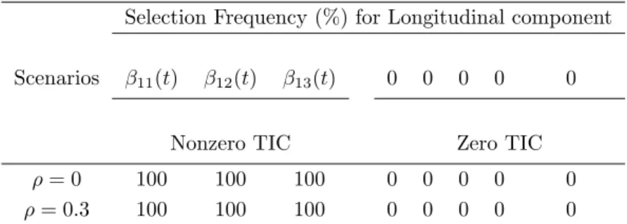
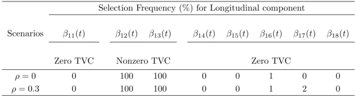
4.1 Selection frequency of time-invariant coefficients (TIC) . . . 80

4.2 Selection frequency of time-varying coefficients (TVC) . . . 81

4.3 TAISE in longitudinal and survival components for time-varying

coeffi-cients . . . 81

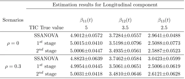
4.4 Estimation results of nonzero time-invariant coefficients (TIC) . . . 82

(11)

LIST OF FIGURES

2.1 Residual plots for data application diagnostics. The circles are the

stan-dardized residuals. The black lines are the LOESS estimates. . . 41

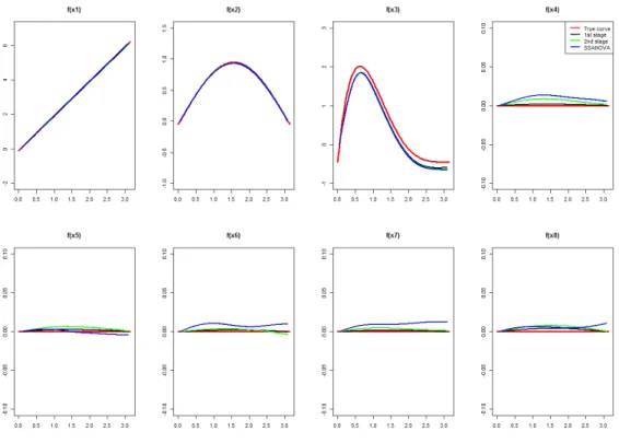
3.1 Curve estimates in the longitudinal component for Scenario 1. . . 63

3.2 Curve estimates in the survival component for Scenario 1. . . 63

3.4 Curve estimates in the survival component for Scenario 2. . . 64

(12)

Chapter 1

Introduction

Statistical modeling has played an increasingly important role in modern scientific investiga-tion. In biomedical research, a significant number of discoveries were made using innovative analytical models. But the validity of model-based scientific inquiry is usually contingent on the correct specification of the model. Failure to include relevant independent variables, for example, will result in questionable inference, while including irrelevant variables cre-ates numerical instability and reduces analytical efficiency. Determination of the correct model structure based on observed data has therefore become an essential component of the modeling process. Ultimately, one hopes to achieve a parsimonious modeling structure without sacrificing predictive or explanatory power.

The objective of this dissertation is to develop a set of model selection tools for joint models of longitudinal and survival outcomes. In this chapter, I present my research ques-tions, review the existing literature, and describe the general approach that I use in this research.

1.1 Joint Models of Longitudinal and Survival Outcomes

The concept of joint models was first proposed by Tsiatis and colleagues to characterize the longitudinal relationship between a disease marker and a time-to-event process (Wulf-sohn and Tsiatis, 1997). Early applications of such models include HIV clinical trials that prospectively measure CD4 counts (or viral loads) and disease mortality (De Gruttola and Tu, 1994; Tsiatis et al., 1995). Here the repeatedly assessed CD4 counts are treated as

(13)

lon-with the purpose of better delineating the relationship between the two. A similar approach is used in studies of prostate cancer, where repeatedly measured prostate-specific antigen (PSA) levels are used as longitudinal outcomes and time to disease reoccurrence is used as the survival outcome (Wulfsohn and Tsiatis, 1997; Xu and Zeger, 2001a).

Joint models, in comparison with the traditional analysis of modeling one outcome at a time, represent a significantly improved analytical approach. Among other things, it affords an opportunity to investigate the intercorrelation, or mutual influences, of the longitudinal and survival outcomes. In aforementioned HIV example, counts of CD4 lymphocytes in-dicate the strength of host immunity against infectious pathogens, thus could be directly related to patient mortality, which in turn censors the CD4 measurement. Failure to ac-commodate the interdependency of the two outcomes thus not only deprives the possibility of exploring the between-outcome association, but also introduces additional biases in es-timation in the presence of measurement errors and early study dropout, especially if the latter is caused by disease exacerbation as reflected by CD4 counts (Tsiatis and Davidian, 2004). To understand the limitations of the separate modeling approach, one only has to look at the traditional two-stage modeling process. In the first stage, a linear mixed-effects model is used to determine the mean levels of the longitudinal outcome; in the second stage, the predicted values from the longitudinal model in the first stage are fed into the survival model. Since deceased patients may have a different longitudinal outcome trajectory, com-pared to those who survived, the two-stage modeling approach could introduce a significant amount of bias into the estimation.

It is from this context that joint models are developed as an alternative modeling strat-egy. By simultaneously accommodating both outcomes, joint models create a structure that retains the natural correlations between the outcomes, thus alleviating the bias due to in-formative missing such as early study dropout. In practice, this implies improved prediction

(14)

accuracy of survival outcome based on longitudinal measurements. As noted in previous research, joint models generally have better efficiency in parameter estimation (Faucett and Thomas, 1996).

To link the two outcomes together, one often resorts to the use of a “shared latent pro-cess” (Wulfsohn and Tsiatis, 1997). For example, in the context of HIV study, the shared latent process is typically thought of as an unobserved disease progress that determines both host immunity (or disease severity), as indicated by CD4 counts, and risk of mortality. By depicting the latent process with a set of random effects and letting them be shared by longitudinal and survival models, one connects the two models and introduces a patient-specific measure of frailty. Such a joint model formulation has been successfully used in many clinical investigations and it is increasingly being recognized as a mainstay analytical method. Early application of joint model mainly focused on the HIV/AIDS trials (De Grut-tola and Tu, 1994; Tsiatis et al., 1995), which remains an important tool in this area (Wu et al., 2010). Another major application of the joint model is in the area of oncology trials to evaluate the association between a patient’s quality of life and time to event end point (Ibrahim et al., 2010), or in the cancer vaccine trials, to investigate the correlation between repeatedly measured immunologic outcomes and patients’ survival outcomes, for example, patients’ time to relapse (Brown and Ibrahim, 2003).

A practical barrier for a more widespread use of this effective analytical approach is the lack of tools for model construction. Specifically, there is no specific guidance on the inclusion and exclusion of independent effects (both fixed and random), the determination of the functional forms of which the independent variables take, and the inclusion of time interactions. In practice, these important questions are left to the analyst, who usually decides in an empirical fashion. Conflicting results may arise as a consequence.

(15)

Methodologically, there is no systematic study of model selection in a joint model setting. Determination of an appropriate model structure is by no means trivial, even in traditional model settings. The joint model structure has significantly magnified the challenge. The goal of this dissertation is to develop a new class of methods for constructing valid joint models. My research consists of three independent but interrelated topics: (1) Fixed and random effect selection; (2) Determination of functional form of an independent variable,

also known as structural discovery; and (3) Selection of time-varying coefficients. The

ultimate goal is to produce a set of data-driven tools to assist analysts construct joint models of longitudinal and survival outcomes.

1.2 Simultaneous Variable Selection

Variable selection has long been viewed as a necessary safeguard for model validity. In a joint model, variable selection has taken on an additional importance of justifying the simultaneous modeling formulation by testing the existence of the shared latent processes, as embodied by the random effects. As a result, variable selection for joint models typically includes the selection of both fixed and random effects.

Existing approaches for variable selection. There is a sizable literature on variable selec-tion in generalized linear models and proporselec-tional hazard model settings. There are three general approaches for variable selection. First, a traditional method is to exhaustively compare all possible models based on a predefined criterion, typically an information-based criterion, such as the Akaike information criteria (AIC, Akaike 1974) or Bayesian informa-tion criterion (BIC, Schwarz 1978). This approach has been used widely in the last several decades and a number of statistical tests, such as the likelihood ratio test, wald-type test, or score test have been derived for variable selection, most notably in less complicated modeling settings. A clear limitation of this approach is that the heavy computational

(16)

burden of fitting of all candidate models. Perhaps for this reason, the method has never been extended to the joint modeling setting. The second approach is the stepwise variable selection method. Although it is computationally more efficient than the first approach, it does not search the entire model space, thus leaving open the possibility that the true model could be missed. When the stepwise approach is applied to mixed-effects models, the alternating procedure of fixing either the mean model for the fixed effects or the covari-ance structure for the random effects yields no unified tests for both types of effects. This could lead to erroneous results as it makes assumptions about the model by fixing part of its structure. An ideal variable selection method for selecting fixed and random effects is to simultaneously select the two parts and search though the full model space. The third approach is the penalized likelihood method. This is a data-driven method requiring less model assumptions and is computationally more efficient, and can perform simultaneous selection of fixed and random effects in a unified framework.

Penalized likelihood method. In this research, I take the third approach - penalized likelihood method - for variable selection in the joint modeling setting. Briefly, the penalized likelihood approach was proposed in the mid-1990’s by Tibshirani (1996). He proposed a least absolute shrinkage and selection operator (LASSO) for fixed-effect variable selection. The “oracle” properties of the smoothly clipped absolute deviation (SCAD; Fan and Li, 2001) and the adaptive least absolute shrinkage and selection operator (ALASSO; Zou, 2006) further strengthened the applicability of this approach. The “oracle” property refers to the consistency between the selected model and the underlying true model. A number of variable selection methods based on the penalized likelihood approach have since been developed for the longitudinal and survival models, although separately. Most of the studies have focused on the selection of fixed effects. Even in the separate models, simultaneous selection of mixed effects presents a formidable challenge. It is not until 2010, simultaneous

(17)

selection of fixed and random effects in a linear mixed model setting has not been resolved (Bondell et al., 2010). More recently, Ibrahim et al. (2011) studied the mixed-effect variable selection in generalized linear mixed models. To the best of my knowledge, no work has been done for simultaneous selection of fixed and random effects in the joint model setting. Variable selection in joint models. The first part of my dissertation concerns the devel-opment of a variable selection method to simultaneously select the mixed effects in a joint model setting. All things considered, this is not a trivial extension of the previous work, as the joint model structure is much more complicated than the separate model. The approach will clearly identify the connections between the two model components, and to simultane-ously select the mixed effects in the two components of the joint model. I reparameterize the joint model to achieve the goal of selection by using a penalized likelihood method.

1.3 Structural Discovery for Joint Models

A logical question following variable selection is what functional form should a variable take. Traditionally, all variables enter the model in a linear form, despite the fact that in biological science, few factors have truly linear influences. I therefore ask how should one determine the functional form of an independent variable? Should an effect be linear, nonlinear, or partially linear? Linear effects are commonly assumed for convenience of model fitting and result interpretation. But modeling a nonlinear effect as linear is a form of model misspecification and may result in erroneous inference. On the other hand, specifying a linear effect using splines or other nonparametric techniques while the true effect is linear will result in reduced efficiency and difficulty in model interpretation.

A valid and efficient regression model requires correct specification of the effect pattern for each independent variable. If an independent variable has a linear effect, one would like to model it as such. Otherwise, if an independent variable’s effect is nonlinear, one

(18)

wants to model it nonparametrically. A data-driven approach to the nonlinearity in an independent variable is often referred to as “structural discovery”. Extensive studies have been done on estimating parameters in a pre-specified linear or nonlinear model, in the separate longitudinal or survival model settings. However, few studies have attempted to detect nonlinearity for the purpose of specifying the functional form of an independent variable. More recently, Zhang et al. (2011) proposed a method for structural discovery in a partially linear model setting.

To ensure the validity of statistical inference, structural discovery procedures are needed for joint models. Extensive literature search suggests that no work has been done in this front. Given its complicated model structure, an ideal simultaneous structural discovery tool should require minimal assumptions and must be implementable without exorbitant computing resources. The second part of my dissertation focuses on this task.

1.4 Selection of Time-Varying Coefficients

Time-varying coefficient models. A more recent extension of linear regression is the ad-dition of time-varying coefficient, which depicts the effect of an independent variable on the outcome not as a constant but as a function of an independent variable (Hastie and Tibshirani, 1993). Such an extension has greatly enhanced the modeling flexibility and has been used to discover important, but nonlinear, biological influences that would have been missed by traditional analysis. For example, the effect of sodium-retaining hormone aldosterone on blood pressure may be dependent on the prevailing levels of extracellular fluid volume, as reflected by plasma renin activity. Varying coefficient model provides a flexible modeling framework to accommodate such interacting influences (Tu et al., 2014). But more often, the effects of certain independent variables on the outcome change over

(19)

gives rise to time-varying coefficient models. Similarly, in survival analysis, one often has the need to model the time-dependent effect of an independent variable. For example, in an analysis of sexually transmitted infections, Yu et al. (2012) showed the effect of number of partners on infection acquisition tended to be age-dependent. In a childhood asthma study, the effect of airway reactivity measurement on the risk of wheezing also changed over time due to child growth (Yu et al., 2013).

Popular estimation methods for time-varying coefficients include kernel based local like-lihood, smoothing spline and B-spline (Yan and Huang, 2012). Although the time-varying coefficient could uncover the temporal pattern of an independent variable effect, unnec-essary nonparametric estimation makes it difficult to interpret the model and also lose some model efficiency. If the independent variable effect is constant over time, the model with time-invariant coefficients is more favorable for better interpretability and increased efficiency.

Selecting time-varying coefficient in joint models. In joint models, independent variables could interact with time, creating a need for time-varying coefficient, although the effects of the same independent variable on the two outcomes could take different functional forms. A statistical tool that helps to determine the functional forms would be very useful in such a modeling situation. Specifically, the tool should be able to consistently distinguish the independent variables with time-invariant or time-varying coefficients.

Model selection tools for time-varying coefficient model is in general limited. For longitu-dinal study, Wang et al. (2008) proposed a penalized likelihood method with SCAD penalty on the expanded nonparametric basis functions of coefficients. For the survival analysis, Yan and Huang (2012) proposed to use ALASSO to select time-invariant and time-varying coefficients, as well as excluding the zero coefficients in the Cox model. Careful literature search does not yield published work in selection of time-varying coefficient in joint model

(20)

settings. I therefore focus on the development of such a procedure in the third part of my dissertation.

(21)

Chapter 2

Selection of Fixed and Random Effects

2.1 Introduction

Longitudinal and survival data often arise together in clinical investigations. In a given subject, longitudinally measured clinical markers and patient survival are usually governed by the same latent disease process, and thus are correlated. Separate modeling for the longitudinal and survival outcomes could result in biases in parameter estimation (Faucett and Thomas, 1996). Joint models are therefore recommended to alleviate biases and to ensure valid inference concerning the correlation structure between the two outcomes. In the past two decades, joint models have been studied extensively: Wulfsohn and Tsiatis (1997) proposed a general framework in which the survival component was depicted by a proportional hazard model, and the longitudinal component was accommodated by a linear-growth-curve model. This basic structure was later extended by Xu and Zeger (2001b) to a variety of data situations. Other noteworthy method developments and significant data applications were presented by De Gruttola and Tu (1994), Nathoo and Dean (2008) and Albert and Shih (2010). Notably missing in this literature is variable selection. As in any modeling exercise, correct specification of the model and inclusion of the right independent variables are of essential importance, for the preservation of scientific validity. For joint models in particular, random variable selection serves the purpose of justifying the use of shared random effects connecting the longitudinal and survival components.

Traditionally, variable selection has been performed through model comparisons using information-based criteria, such as the Akaike and Bayesian information criteria (AIC and

(22)

of candidate models is large. As an alternative, penalized likelihood approach has gained popularity since the mid-1990’s. Tibshirani (1996) proposed a least absolute shrinkage and selection operator (LASSO) for fixed-effect selection. Asymptotic “oracle” properties of the smoothly clipped absolute deviation (SCAD; Fan and Li, 2001) and the adaptive least absolute shrinkage and selection operator (ALASSO; Zou, 2006) have provided a theoretical assurance for mixed-effect selection. Along this line, Fan and Li (2004), Garcia et al. (2010)

and Johnson et al. (2008) discussed the application of penalized likelihood method to

select fixed effect variables in longitudinal model settings. Fan and Li (2002), Garcia et al. (2010) and Zhang and Lu (2007) discussed the selection of fixed effects in survival models. Extending these previous work, Bondell et al. (2010) proposed a method for selecting fixed and random effects in a linear mixed-effects model setting. Most recently, Ibrahim et al. (2011) studied the mixed-effects selection in generalized linear mixed models through an EM algorithm. To the best of our knowledge, no work has been done for simultaneous selection of fixed and random effects in a joint model setting with longitudinal and survival outcomes. To fill in this methodological gap, I propose a penalized likelihood method with ALASSO penalty for fixed and random effect selection in joint models. I optimize the penalized likelihood using an EM algorithm.

I illustrate the method by analyzing data from an observational study of heart failure patients. The study cohort included 1702 patients with diagnosed congestive heart failure (CHF) between Jan 1, 2004 and Dec 31, 2009, identified from a large electronic medical record system. The analytical objective is to assess the effects of medication adherence on disease exacerbation and on patient survival; I also like to assess the correlation between

CHF exacerbation and patient mortality. Specifically, I considered two outcomes: the

survival outcome is defined as the time from the first recorded CHF diagnosis to mortality, or to Dec 31, 2009, which ever comes first; the longitudinal outcomes are the repeatedly

(23)

measured B-type natriuretic peptide (BNP) levels. BNP is a commonly used bedside marker of CHF exacerbation; a higher BNP value indicates fluid volume overload in the left ventricle and increased mortality risk. (Morrison et al., 2002). Although the two outcomes can be modeled individually, separate modeling does not accommodate correlations between

BNP and survival. In this research, I consider a joint modeling approach. I consider

eight known risk factors and four interaction terms as candidate variables and develop an ALASSO procedure to select the independent variables. In particular, I consider random-effect selection as medical literature rarely avails information on the possible random slopes (e.g., the effect of an independent variable varies across subjects). Misspecification of fixed and random effects for the two outcome variables could result in erroneous inferences.

2.2 Method

2.2.1 Model Formulation

Suppose in a longitudinal study, I observe a survival outcome (ti, δi), and repeated

mea-surements of a continuous outcome yi, for subject i = 1,· · · , n. Here ti is the observed

event time subject to right censoring, andδi is a failure indicator withδi= 1 indicating the

occurrence of an event of interest, and δi = 0 indicating censoring, whereasyi is an ni×1

vector of the ni repeated measurements. Let X1i ∈ Rni×p and Z1i ∈ Rni×q be the fixed

and random covariate matrices for the longitudinal outcome, respectively. Similarly, I let

x2i ∈Rp1 andz2i ∈Rq1 be the fixed and random covariate vectors for the survival outcome.

Combining these observations I write Oi = (yi,X1i,Z1i, ti, δi,x2i,z2i). I assume that the

observationsOi are independent across subjects.

Without loss of generality, I herein consider a case where the longitudinal and survival components share the same set of fixed- and random-effect covariates. This model

(24)

formula-tion could easily be generalized to situaformula-tions where the two components have different sets of covariates.

For the longitudinal outcome, I consider the following linear mixed-effects model:

y_i=X1iβ1+Z1iΓ1bi+εi, (2.1)

where β₁ = (β10, β11, . . . , β1p)T is the coefficient vector, and β10 is the intercept. εi =

(εi1,· · ·, εini)

T _∼_N

ni(0, σ

2_I

ni) is the measurement error vector, andbi∈R

q

1 is a

q−dimensional random effect vector following a multivariate normal distributionNq(0,Iq),

with Iq as a q×q identity matrix. Γ1 is a q×q lower triangular matrix and Γ1bi follows

Nq(0,D1). ThusΓ1 represents a Cholesky decomposition of the covariance matrix D1.

For the survival outcome, I consider a frailty model, defined as follows:

h(ti) =h0(ti) exp(x2iβ2+z2iΓ2bi), (2.2)

where h0(ti) is the baseline hazard function, and β2 = (β21, . . . , β2p)T is the coefficient

vector. Γ2bi followsNq(0,D2), andΓ2 is a Cholesky decomposition of theq×q matrixD2.

2.2.2 Variable Selection Using Penalized Likelihood

To select fixed and random effects, I propose a penalized likelihood to simultaneously

iden-tify the non-zero elements in (β₁,β₂,Γ1bi,Γ2bi). Let θ = (β1,β2,Γ1,Γ2,φ) be the

collec-tion of all the unknown parameters, whereφdenotes parameters other than (β₁,β₂,Γ1,Γ2).

Writing the density function of (yi, ti,bi) asf(yi, ti,bi|X1i,Z1i,x2i,z2i, h0(ti), δi,θ), I have

the following log-marginal likelihood forθ:

lo(θ) = n X log Z fy(yi|X1i,Z1i,bi,θ)fs(ti, δi|x2i,z2i, h0(ti),bi,θ)fb(bi)dbi, (2.3)

(25)

where fb(bi) is a q−variate normal density function for bi. Functions fs(·) and fy(·) are the conditional density functions of the survival time and repeated measurements when

bi is given, respectively. I note that in the absence of restrictions on the baseline hazard

h0(ti), the maximum of the marginal likelihood is infinity. To remedy the deficiency, one

could parameterizeh0(ti) with a parametric distribution. For example, a natural choice is

to use a Weibull distribution with a baseline hazard h0(ti) =αλtαi−1, whereα is the shape

parameter andλis the scale parameter. Alternatively, one could use a piece-wise constant

baseline hazard by dividing the study period into m intervals and assuming h0(t) to be a

constant within each interval ash0(t) =hk, tk−1 < t≤tk, k= 1. . . m, where tks are knots

defining the intervals. This piece-wise constant baseline hazard have been shown to perform well by Feng et al. (2005).

To select fixed and random effects simultaneously, I consider a penalized likelihood

P L(θ) = _n1lo(θ)−κλ1(β1)−κλ2(β2)−κλ3(D1)−κλ4(D2). The penalty terms κλ1(β1)

and κλ2(β2) control for the sparsity of estimates ofβ1 andβ2 so that the fixed effects are

selected. The penalty terms κλ3(D1) andκλ4(D2) control for the sparsity of estimates of

D1 and D2 to select the random effects. The penalty functions κλj(·), for j = 1,2,3,4,

could be the adaptive LASSO, or the smoothly clipped absolute deviation (SCAD). For the

fixed-effect selection, I define the adaptive LASSO penalties asκλ1(β1) =λ1

Pp

j=1ωβ1j|β1j|

and κλ2(β2) =λ2

Pp

k=1ωβ2k|β2k|, where λ1 and λ2 are tuning parameters that control the

degree of penalties;ωβ1j, ωβ2k are the corresponding positive weights for penalties|β1j|and

|β₂_k|. The summation in κλ1(β1) = λ1

Pp

j=1ωβ1j|β1j|starts from 1 as I am not interested

in selecting interceptβ10. Some of the estimates of ˆβ1j and ˆβ2k will be zero since|β1k|and

|β2k|are singular when|β1j|= 0 and|β2k|= 0.

For the random-effect selection, I note that D1 = Γ1ΓT1 and D2 = Γ2ΓT2. Let γ1m

(26)

and γ₂_lγT₂_l =D2ll are the variance components of themth and lth elements of the random

effects Γ1bi and Γ2bi. I form the penalty terms for the random effects in a group manner

so that the estimates of elements of the entire vectors γ₁_m and γ₂_l are either all zero or

at least one of the estimates is non-zero. The group penalties on γ1m and γ2l will ensure

selection for the covariance structure due to the following connection of covariance matrices

D1, D2 and the Cholesky decomposition matricesΓ1,Γ2 (Wang et al., 2010):

γ1m = 0⇔D1mm= 0, D1mh=D1hm= 0, ∀h

γ2l = 0⇔D2ll= 0, D2lh=D2hl = 0, ∀h.

(2.4)

From (2.4), it follows that ifγ1m = 0, then the diagonal elementD1mm, the variance of

the random effect (Γ1bi)m, is zero. Furthermore, for any h6=m, the off-diagonal element

D1mh=D1hm= 0 implies that the covariance between (Γ1bi)mand all other random effects

are zero. Thus, the random effect (Γ1bi)m in longitudinal component is to be excluded from

the model and the positive-definiteness ofD1will be preserved. This applies to the

random-effect selection in the survival component as well, which is to shrink the whole vector γ2l

to zero.

To perform group penalties on vectors γ1m and γ2m, I first summarize the penalties

using L2−norm: ||γ1m|| = (γ1mγT1m)1/2 and ||γ2l|| = (γ2lγT2l)1/2 for m, l= 2,· · · , q.

Fol-lowing Yuan and Lin (2006), the adaptive LASSO penalties are defined as: κλ3(D1) =

λ3Pq_m₌₂ωγ1m||γ1m|| and κλ4(D2) = λ4

Pq

l=2ωγ2l||γ2l||. I use adaptive LASSO penalties

in the simulation study. Note that the summation starts from m= 2, l= 2, as I keep the

random intercepts in both the longitudinal and survival components without eliminating the

possible minimal within-cluster correlation. λ3 and λ4 are the positive tuning parameters,

and ωγ1m, ωγ2l, are the positive weights associated with penalties on||γ1m||and||γ2l||. Let

p(θ) =λ Pp

ω |β |+λ Pp

ω |β |+λ Pq

ω ||γ ||+λ Pq

(27)

and the penalized likelihood with the adaptive LASSO penalties can be written as

pl(θ) = 1

nlo(θ)−p(θ). (2.5)

Penalized likelihood with SCAD penalties could be constructed by substituting the

penalty terms in (2.5) using SCAD. The estimator of θ can be obtained by maximizing

(2.5).

2.2.3 EM Algorithm for Optimization of the Penalized Likelihood

To maximize the penalized likelihood (2.5), I use an EM algorithm. I start with the penalized

log-complete likelihood for (Oi,bi) for i= 1,· · · , n, which is

plc(θ) = 1 n n X i=1 logf(y_i, ti, δi,bi|θ)−p(θ) =1 n n X i=1

{log[fy(yi|bi,θ)] +δilog[h(ti|bi,θ)] + log[S(ti|bi,θ)] + log[fb(bi|θ)]} −p(θ).

(2.6)

In Equation (2.6), S(·) is the survival function of ti conditional on bi. Let λ =

(λ1, λ2, λ3, λ4)T and ω= (ωβ1j, ωβ2k, ωγ1m, ωγ2l)

T_{. I denote}_g

c,i1 = (yi,X1i,Z1i,bi),gc,i2=

(ti, δi,x2i,z2i,bi) and gc,i = (yi,X1i,Z1i, ti, δi,x2i,z2i,bi) as the complete data for

lon-gitudinal, survival and both components, respectively, and g_o,i₁ = (y_i,X1i,Z1i), go,i2 =

(ti, δi,x2i,z2i) and go,i= (yi,X1i,Z1i,x2i,z2i) as the corresponding observed data.

E-step

I first derive the E-step of the EM algorithm for the givenλ and ω. Assuming that I have

estimatesθ(s) from the (s)th iteration of the maximization step, I take the expectation of

(28)

the following penalized Q-function: Qλ,ω(θ|θ(s)) = 1 n n X i=1

{E[logfy(gc,i1,θ)|(go,i,θ(s))] +E[δilogh(gc,i2,θ)|(go,i,θ(s))]

+E[logS(g_c,i₂,θ)|(g_o,i,θ(s))]} −p(θ) + 1

n n X i=1 E[logfb(bi)|(go,i,θ(s))]. (2.7) I write E[H(bi)|(go,i,θ(s))] = Z H(bi)fb(bi|go,i,θ(s))dbi, (2.8)

for each of H(bi) = logfy(gc,i1,θ), H(bi) = δilogh(gc,i2,θ), and H(bi) = logS(gc,i2,θ).

Because integral (2.8) is intractable, I approximate it by using a multivariate Gaussian

quadrature method (Pinheiro and Bates, 1995). Since bi ∼N(0,Iq), if I choosek

quadra-ture points in each dimension, there will be kq vector nodes of q ×1 dimension. Let

b0_l = (b0_l,₁, b0_l,₂,· · ·, b0_l,q) denote the lth node, and wl denote the corresponding quadrature

weight, forl= 1,· · ·, kq, integral in (2.8) can be approximated by

˜ E{H(bi)|(go,i,θ(s))} ≈ kq X l=1 wlH(b0_l)fb(b0_l|go,i,θ(s)). (2.9)

I therefore obtain the approximated penalized Q-function in the (s+ 1)th iteration

˜ Qλ,ω(θ|θ(s)) = 1 n n X i=1

{E˜[logfy(gc,i1,θ)|(go,i,θ(s))] + ˜E[δilogh(gc,i2,θ)|(go,i,θ(s))]

+ ˜E[logS(g_c,i₂,θ)|(g_o,i,θ(s))]} −p(θ).

(2.10)

The last term _n1Pn

i=1E[logfb(bi)|(go,i,θ(s)) in (2.7) does not involve any unknown

(29)

M-step

I maximize (2.10) with respect to the fixed- and random-effect parameters alternatively.

When (Γ1,Γ2, φ) are fixed, I maximize (2.10) with respect to (β1,β2), and the penalty

function involvingL1 penalty terms can be solved by applying the LARS/LASSO algorithm

(Efron et al., 2004) and the SCAD penalties could be solved according to Fan and Li (2001).

When (β₁,β₂,φ) are fixed, I maximize (2.10) with respect to(Γ1,Γ2). Following Lin and

Zhang (2006) and Wang et al. (2010), I transform the optimization problem to a two-step equivalent objective function involving quadratic penalty term that is easier to solve. Specifically, let ˜ Q(θ|θ(s)) =1 n n X i=1

{E˜[logfy(gc,i1,θ)|(go,i,θ(s))] + ˜E[δilogh(gc,i2,θ)|(go,i,θ(s))]

+ ˜E[logS(g_c,i₂,θ)|(g_o,i,θ(s))]},

then for any given βˆand (λ, ω), the following two optimization problems with respect to

γs achieve the same solution:

˜ Q(β,ˆ Γ1,Γ2|θ(s))−λ3 q X m=2 ωγ1m||γ1m|| −λ4 q X l=2 ωγ2l||γ2l|| (2.11) ˜ Q(β,ˆ Γ1,Γ2|θ(s))− q X m=2 ζ₁2_m−1 4 q X m=2 (λ3ωγ1m) 2 ζ2 1m ||γ1m||2− q X l=2 η₂2_l−1 4 q X l=2 (λ4ωγ2l) 2 η2 2l ||γ2l||2. (2.12)

Let (γˆ₁_m,γˆ₂_l) be the maximizer of (2.11), and ( ˜ζ1m,γ˜1m,η˜2l,γ˜2l) be the maximizer of

(2.12), then I have ˆ γ1m = ˜γ1m,γˆ2l = ˜γ2l (2.13) ˜ ζ1m= r λ3ωγ1m 2 ||ˆγ1m||,η˜2l= r λ4ωγ2l 2 ||ˆγ2l||. (2.14)

(30)

Equations (2.13) and (2.14) imply that one can optimize (2.12) iteratively with respect

to (γ1m,γ2l) and (ζ1m, η2l), instead of directly maximizing (2.12). Maximizing (2.12) with

respect to (γ1m,γ2l) when (ζ1m, η2l) is given is similar to a generalized ridge regression.

When (γ1m,γ2l) is given, (ζ1m, η2l) could be easily computed from (2.14).

Let Θ = (θ, ζ1m, η2l), where θ = (β1,β2,Γ1,Γ2,φ) are defined in section (2.2.2). I

propose the expectation conditional maximization procedures to optimize the penalized likelihood as follows:

1. Initialize (β(0)₁ ,β₂(0),γ₁(0)_m, ζ₁(0)_m,γ₂(0)_l , η(0)₂_l ,φ(0)_{) with some plausible values.}

2. For iteration s, updateβ1,β2 by adaptive LASSO,

β1(s),β2(s) =argmax β1,β2 ˜ Q(β1, β2,Γˆ₁(s−1),Γˆ(₂s−1),φˆ(s−1)|βˆ₁(s−1),βˆ₂(s−1), ˆ Γ₁(s−1),Γˆ₂(s−1),φˆ(s−1))−λ1 p X j=1 ωβ1j|β1j| −λ2 p X k=1 ωβ2k|β2k|. 3. Updateγ1m,γ2l: γ1m(s),γ2l(s)=argmax γ1m,γ2l ˜ Q(βˆ₁(s),βˆ(₂s),Γ1,Γ2,φˆ(s−1)|βˆ(1s),βˆ (s) 2 ,Γˆ (s−1) 1 ,Γˆ (s−1) 2 ,φˆ(s −1)₎ −1 4 q X m=2 (λ3ωγ1m) 2 (ζ₁(s_m−1))2 ||γ1m|| 2₋1 4 q X l=2 (λ4ωγ2l) 2 (η(₂s_l−1))2 ||γ2l|| 2_. 4. Updateζ1m, η2l: ζ₁(s_m) = r λγ1ωγ1m 2 ||γ (s) 1m||, η (s) 2l = r λγ2ωγ2l 2 ||γ (s) 2l ||. 5. Updateφ: φ=argmax φ ˜ Q(βˆ(₁s),βˆ₂(s),Γˆ(₁s),Γˆ₂(s),φ|βˆ₁(s),βˆ(₂s),Γˆ(₁s),Γˆ(₂s),φˆ(s−1)).

(31)

6. Terminate the iteration when max|Θ(s)₋_Θ(s−1)_| _{are small enough. Otherwise, let}

s=s+ 1 and go back to step 2.

Before updating parameters in each step, the corresponding ˜Qfunction is approximated

by Gaussian quadrature in the E-step. To improve computation stability, smaller subset of

(β₁,β₂,Γ1,Γ2,φ) could be updated iteratively. I could update β1 when (β2,Γ1,Γ2,φ) is

fixed, and then updateβ₂ when (β₁,Γ1,Γ2,φ) is fixed, and sequentially for Γ1,Γ2, andφ

when other parameters are fixed. It is at the price of more iterations. The typical values

for the weights are selected as: ωβ1j =|βˆ

∗ 1j|−1, ωβ2k =|βˆ ∗ 2k|−1, ωγ1m = √ m||ˆγ1m∗||−1, ωγ2l= √ l||ˆγ2l∗||−1, where ˆβ1∗j,βˆ ∗

2k,γˆ1m∗,ˆγ2l∗ are the unpenalized MLEs (Ibrahim et al., 2011;

Zou, 2006) and √m,√l are the normalizing constants for penalty parameters γ1m, γ2l to

accommodate the varying sizes of γ1m,γ2l.

2.2.4 Tuning Parameter Selection and Two-stage Estimation

A data-driven method for determining tuning parameters is essential for variable selection. Criteria such as generalized cross-validation, k-fold cross validation, AIC, BIC, or GIC have been used as the objective scores to minimize over a preselected grid of tuning parameters. BIC is known to be consistent in the model selection (Pu and Niu, 2006; Shao, 1997). Wang et al. (2009) showed that selecting tuning parameters via BIC consistently yielded the true model in the linear model setting. Ibrahim et al. (2011) showed that selecting tuning

parameters for mixed-effects selection via BIC-typeICQ criterion also consistently yielded

true models in generalized linear mixed models; their simulation study further showed that the approach worked well in finite sample situations. Thus, I propose to use the BIC-type criterion to determine the values of tuning parameters, where

(32)

In (2.15), θˆare the estimators obtained from penalized likelihood under the given λ, and

lo(θˆ) is the value of the observed likelihoodlo(θ) at the estimatesθˆ. The solution is chosen

to minimize theBICλ criterion. In this BIC-type criterion, the total sample sizenis used.

I take d, the total number of non-zero estimates of ˆθ as the degree of freedom dfλ. In the

linear model, dis an unbiased estimator of dfλ. Our simulation shows this criterion works

well, as suggested by Pu and Niu (2006).

To reduce the estimation bias, I propose a two-stage process. In the first stage, I focus on variable selection and use the penalized likelihood method to select the model that minimizes the BIC value. In the second stage, I re-estimate parameters using selected variables without penalty for selection, to reduce the estimation bias.

2.3 Simulation Study

2.3.1 Data Generation

I conduct a simulation study to examine the performance of the proposed method. I generate data under six different scenarios.

For Scenarios 1 to 4, I generate the longitudinal outcome Yij from the following model:

Yij =1 + 1X1ij,1+ 0X1ij,2+ 3X1ij,3+ 0X1ij,4+bli,0

+bli,1Z1ij,1+bli,2Z1ij,2+bli,3Z1ij,3+bli,4Z1ij,4+ij,

(2.16)

and the failure time from a Weibull distribution with the hazard function:

λi(t) =λ0(t) exp(1x2i,1+ 0x2i,2+ 0x2i,3+ 1x2i,4

+bsi,0+bsi,1z2i,1+bsi,2z2i,2+bsi,3z2i,3+bsi,4z2i,4),

(2.17)

(33)

Random effect vectorbiis independently generated fromN(0,I5). bli= (bli,0, bli,1, bli,2,

bli,3, bli,4) is obtained frombli= Γ1bi andbsi = (bsi,0, bsi,1, bsi,2, bsi,3, bsi,4) is obtained from

bsi= Γ2bi, whereΓ1=σDR1 and Γ2 =σDR2, with lower triangular matrix

R1 =                                      1 0 0 0 0 1 2 1 2 0 0 0 0 0 0 0 0 1 4 1 4 1 4 1 4 0 0 0 0 0 0                                      1 2 and R2=                                      1 0 0 0 0 1 2 1 2 0 0 0 0 0 0 0 0 0 0 0 0 0 1 5 1 5 1 5 1 5 1 5                                      1 2

CovariatesX1ij,1 =Z1ij,1, X1ij,2 =Z1ij,2, X1ij,4=Z1ij,4andx2i,1 =z2i,1, x2i,2 =z2i,2, x2i,4=

z2i,4 are generated as independent N(0,1) variables; X1ij,3 = Z1ij,3 and x2i,3 = z2i,3

are binary variables with equal probability taking value 0 or 1. The measurement error

ij ∼ i.i.d.N(0,1). Censoring time is independently generated from an exponential distri-bution to achieve the desired censoring percentage.

In Scenario 1, I set σD to

√

0.5 and censoring percentage to 30%; in Scenario 2, I set

σD to √

1 and censoring percentage to 30%; in Scenario 3, I set σD to

√

0.5 and censoring

percentage to 10%; in Scenario 4: I setσD to

√

(34)

I additionally simulate data settings where there are higher proportions of censoring (Scenario 5) and larger numbers of random effects (Scenario 6). For scenario 5, I generate

the longitudinal outcome Yij from the following model:

Yij =1 + 1.5X1ij,1+ 2X1ij,2+ 0X1ij,3+ 0X1ij,4+bli,0

+bli,1Z1ij,1+bli,2Z1ij,2+bli,3Z1ij,3+bli,4Z1ij,4+ij,

λi(t) =λ0(t) exp(1.5x2i,1+ 2x2i,2+ 0x2i,3+ 0x2i,4

+bsi,0+bsi,1z2i,1+bsi,2z2i,2+bsi,3z2i,3+bsi,4z2i,4),

fori= 1, . . . ,800, j= 1, . . . ,5, whereλ0(t) =αλtα−1 withα= 2, and λ= exp(1) = 2.718.

Random effect bi is independently generated from N(0,I5). bli = (bli,0, bli,1, bli,2,

bli,3, bli,4) is obtained by bli = Γ1bi and bsi = (bsi,0, bsi,1, bsi,2, bsi,3, bsi,4) is obtained by

bsi= Γ2bi, where Γ1 =Γ2=σD                                      1 0 0 0 0 1 2 1 2 0 0 0 1 3 1 3 1 3 0 0 0 0 0 0 0 0 0 0 0 0                                      1 2 and σD = √

0.5. Covariates X1ij,1 = Z1ij,1, X1ij,2 = Z1ij,2, X1ij,3 = Z1ij,3, X1ij,4 = Z1ij,4

andx2i,1=z2i,1, x2i,2 =z2i,2, x2i,3 =z2i,3, x2i,4=z2i,4 are generated as independentN(0,1)

variables; The measurement error ij ∼i.i.d.N(0,1). The censoring time is independently

(35)

In Scenario 6, I generate the longitudinal outcome Yij from the following model:

Yij =1 + 1.5X1ij,1+ 2X1ij,2+ 2.5X1ij,3+ 0X1ij,4+ 0X1ij,5+ 0X1ij,6+ 0X1ij,7+

bli,0+bli,1Z1ij,1+bli,2Z1ij,2+bli,3Z1ij,3+bli,4Z1ij,4+bli,5Z1ij,5+bli,6Z1ij,6+

bli,7Z1ij,7+ij,

λi(t) =λ0(t) exp(1.5x2i,1+ 2x2i,2+ 2.5x2i,3+ 0x2i,4+ 0x2i,5+ 0x2i,6+ 0x2i,7+

bsi,0+bsi,1z2i,1+bsi,2z2i,2+bsi,3z2i,3+bsi,4z2i,4+bsi,5z2i,5+

bsi,6z2i,6+bsi,7z2i,7),

fori= 1, . . . ,250, j= 1, . . . ,5, whereλ0(t) =αλtα−1 withα= 2, and λ= exp(1) = 2.718.

Random effect bi is independently generated from N(0,I8). bli = (bli,0, bli,1, bli,2,

bli,3, bli,4 bli,5, bli,6, bli,7) is obtained bybli= Γ1bi andbsi= (bsi,0, bsi,1, bsi,2, bsi,3, bsi,4, bsi,5,

bsi,6, bsi,7) is obtained bybsi = Γ2bi, where

Γ1=Γ2 =σD                                                                  1 0 0 0 0 0 0 0 1 2 1 2 0 0 0 0 0 0 1 3 1 3 1 3 0 0 0 0 0 1 4 1 4 1 4 1 4 0 0 0 0 0 0 0 0 0 0 0 0 0 0 0 0 0 0 0 0 0 0 0 0 0 0 0 0 0 0 0 0 0 0 0 0                                                                  1 2

(36)

and σD = √

0.5. Covariates X1ij,1 = Z1ij,1, X1ij,2 = Z1ij,2, X1ij,3 = Z1ij,3, X1ij,4 = Z1ij,4,

X1ij,5 = Z1ij,5, X1ij,6 = Z1ij,6, X1ij,7 = Z1ij,7 and x2i,1 = z2i,1, x2i,2 = z2i,2, x2i,3 =

z2i,3, x2i,4 = z2i,4, x2i,5 = z2i,5, x2i,6 = z2i,6, x2i,7 = z2i,7 are generated as independent

N(0,1) variables; The measurement error ij ∼ i.i.d.N(0,1). The censoring time is

inde-pendently generated from an exponential distribution to ahieve a 30% censoring percentage. For each scenario, I generate 100 data sets and apply the proposed method to select the non-zero fixed or random effects in the first-stage model. After obtaining the selected variables, I fit the second-stage model including only the selected effects. The tuning

pa-rametersλ1, λ2, λ3, λ4 are determined by minimizing the BIC criterion, as defined in (2.15).

The model without variable selection is also fitted for comparison.

2.3.2 Simulation Results

For Scenarios 1 to 4, I present the fixed- and random-effect selection results in Table 2.1, fixed-effect estimation results in Tables 2.2 and 2.3, and random-effect estimation results in Table 2.4. For fixed effects, the average correct selection rates are 100% for both non-zero and non-zero effects in longitudinal component, and 100% for non-non-zero and 98% for non-zero effects in survival component. The longitudinal fixed-effect estimates do not show severe biases in the first-stage estimation, and the biases are further reduced to less than 1% in the second-stage estimation. The survival fixed-effect estimates show 15% to 25% biases in the first-stage estimation, and the biases are reduced to below 4% in the second-stage estimation.

For random effects, the average rates of correct selection are 100% for non-zero and 94% for zero effects in longitudinal component, and approximately 96% for non-zero and 90% for zero effects in survival component. For non-zero random effects, the estimates in longitudinal component have biases ranging from 8% to 17% in the first-stage estimation,

(37)

and the biases are reduced to below 6% in the second-stage estimation. The survival non-zero random effect estimates show up to 42% biases in the first-stage estimation; in the second stage, the biases are reduced to less than 8%. For zero random effects, both the first- and second-stage estimates in longitudinal component have biases below 2%. The survival zero random effect estimates generally have less than 10% biases in both stage estimations.

Simulation results for settings with higher proportions of censoring and larger numbers of random effects are reported in Tables 2.5, 2.6, 2.7, 2.8, 2.9 and 2.10. Briefly, I find that the probabilities of correct selection remain excellent for these data settings.

One consequence of including more random effects is the increased computing time. The complexity of Gaussian quadrature increases exponentially with the dimension of the random effect vector. In this research, I used 3 quadrature points. With 3 quadrature points, each data set in Scenarios 1 to 4 took approximately 20 minutes to complete the first stage variable selection under one tuning parameter; and it took another 10 minutes in the second stage estimation. When I increased the number of random effects to 8 (as in Scenario 6), the computation time increased to 10 and 5 hours, respectively. The computing time is estimated on a single CPU (Intel(R) Xeon(R) CPU E7- 4830 @ 2.13GHz) and 4 GB memory in the Unix system. The total computing time depended on the number of tuning parameters. Other factors, such as the shape of the likelihood function could also influence the approximation accuracy of Gaussian quadrature and the computing time.

Generally, mis-selection rate increases as the censoring rate increases or the variance

magnitude σD decreases, since smaller variance σD means less resolution between non-zero

and zero random effects. The mis-selection subsequently leads to larger estimation bias. The influence of censoring rate on selection accuracy is greater than that of variance. Increased number of random effects does not necessarily lead to worse selection accuracy, but it

(38)

tends to slightly increase estimation bias, which may be due to the reduced approximation accuracy of Gaussian quadrature method. The estimates from the model without variable selection generally have more biases than the second-stage estimates, especially for the zero effects. In summary, I contend that the proposed variable selection and estimation method works well even under high proportions of censoring and large number of random effects. The two stage procedure ensures good selection performance in the first stage and reduced biased parameter estimation in the second stage.

(39)

T able 2.1: Selection frequency of mixed effects in longitudinal an d surviv al comp onen ts for Scenarios 1 to 4 Fixed effect selection Sel. F req.(%) for Longitud inal comp onen t Sel. F req.(%) for Surviv al comp onen t Scenarios X1 , 1 X1 , 2 X1 , 3 X 1 , 4 X 2 , 1 X 2 , 2 X 2 , 3 X2 , 4 Non-Zero Zero Non-Zero Zero Non-Zero Zero Zero Non-Zero 1 100 0 100 0 100 1 3 100 2 100 0 100 0 100 3 4 100 3 100 0 100 0 100 0 1 100 4 100 0 100 0 100 1 1 100 Random effect selection Sel. F req.(%) for Longitud inal comp onen t Sel. F req.(%) for Surviv al comp onen t Scenarios Z1 , 1 Z1 , 2 Z1 , 3 Z1 , 4 Z2 , 1 Z2 , 2 Z2 , 3 Z2 , 4 Non-Zero Zero Non-Zero Zero Non-Zero Zero Zero Non-Zero 1 100 8 100 11 99 7 19 84 2 100 2 100 6 100 10 13 92 3 100 2 100 10 100 5 12 97 4 100 1 100 10 100 6 8 99

(40)

T able 2.2: Estimation of fixed effects β1 ,j in longitudinal comp onen t for Scenarios 1 to 4 ˆβ1 ,j ± S E (Co v erage probabilit y) for Longitudinal comp onen t a Scenarios In tercept X1 , 1 X1 , 2 X 1 , 3 X 1 , 4 T rue v alue β 1 1 0 3 0 1 W/O selection ˆβ 1.002 ± 0.076(87%) 1.007 ± 0.075(81%) -0.003 3.009 ± 0.077(96%) 0 .000 1 st stage ˆβ 1.006 ± 0.071(94%) 0.989 ± 0.072(88%) 0.0 00 2.988 ± 0.074(97%) 0 .000 2 nd stage ˆβ 0.999 ± 0.068(95%) 1.003 ± 0.067(85%) 0.0 00 3.003 ± 0.070(98%) 0 .000 2 W/O selection ˆβ 0.995 ± 0.108(76%) 0.998 ± 0.111(66%) -0.005 2.999 ± 0.111(89%) 0 .001 1 st stage ˆβ 1.002 ± 0.099(79%) 0.979 ± 0.103(74%) 0.000 2.979 ± 0.096(89%) 0 .000 2 nd stage ˆβ 0.994 ± 0.108(82%) 0.996 ± 0.108(75%) 0.000 2.997 ± 0.094(94%) 0. 000 3 W/O selection ˆβ 1.000 ± 0.076(84%) 1.005 ± 0.075(80%) -0.003 3.007 ± 0.078(96%) -0.001 1 st stage ˆβ 1.007 ± 0.070(96%) 0.989 ± 0.072(91%) 0.000 2.988 ± 0.074(98%) 0. 000 2 nd stage ˆβ 0.998 ± 0.070(93%) 1.002 ± 0.066(88%) 0.000 3.003 ± 0.07(98%) 0.000 4 W/O selection ˆβ 0.994 ± 0.113(72%) 1.002 ± 0.111(63%) -0.005 3.003 ± 0.109(89%) 0. 001 1 st stage ˆβ 1.004 ± 0.102(85%) 0.983 ± 0.103(78%) 0.000 2.982 ± 0.098(91%) 0. 000 2 nd stage ˆβ 0.995 ± 0.108(81%) 1.000 ± 0.104(73%) 0.000 2.999 ± 0.091(95%) 0. 000 a ˆβs are the a v erages of estimates o v er the 100 data sets; SE is the empirical standard error of the 100 ˆβs ; F or eac h data set, the 95% confidence in terv al base d on the parameter and standard error estimates is calculated and the corresp onding co v erage probabilities for the true v alue o v er the 100 data sets are included in the paren theses. SE and co v erage proba bilit y a re only rep orted for non-zero v ariables.

(41)

T able 2.3: Estimation of fixed effects β2 ,j in surviv al comp onen t for Scenari os 1 to 4 ˆβ2 ,j ± S E (Co v erage probabilit y) for Surviv al comp onen t a Scenarios In tercept X2 , 1 X2 , 2 X2 , 3 X2 , 4 T rue v alue β -1 0 0 1 1 W/O selection ˆβ 1.140 ± 0.275(86%) -0.009 0.010 1.141 ± 0.308(81%) 1 st stage ˆβ 0.854 ± 0.224(59%) -0.001 -0.005 0.853 ± 0.255(62%) 2 nd stage ˆβ 1.000 ± 0.263(89%) 0.001 0.014 0.996 ± 0.285(80%) 2 W/O selection ˆβ 1.110 ± 0.370(79%) -0.023 -0.013 1.137 ± 0.424(79%) 1 st stage ˆβ 0.751 ± 0.312(35%) 0.001 -0.007 0.778 ± 0.348(40%) 2 nd stage ˆβ 0.990 ± 0.417(83%) 0.017 0.015 1.030 ± 0.636(81%) 3 W/O selection ˆβ 1.157 ± 0.256(84%) 0.005 0.040 1.145 ± 0.250(88%) 1 st stage ˆβ 0.878 ± 0.187(63%) -0.001 -0.003 0.876 ± 0.187(66%) 2 nd stage ˆβ 1.023 ± 0.158(98%) 0.000 0.003 1.021 ± 0.161(92%) 4 W/O selection ˆβ 1.113 ± 0.259(84%) 0.000 0.054 1.132 ± 0.299(85%) 1 st stage ˆβ 0.792 ± 0.207(53%) 0.000 0.001 0.810 ± 0.245(51%) 2 nd stage ˆβ 1.008 ± 0.187(91%) 0.003 0.002 1.013 ± 0.239(86%) a ˆβs are the a v erages of estimates o v er the 100 data sets; SE is the empirical standard error of the 100 ˆβs ; F or eac h data set, the 95% confidence in terv al based on the parameter and standard error estimates is calculated and the corresp onding co v erage probabilities for the true v alue o v er the 100 data sets are included in the paren theses. SE and co v erage probabilit y are only rep orted for non-zero v ariables.

(42)

T able 2.4: Estimation of random effects √ D 1 k k and √ D 2 k k in longitudinal and survi v al comp onen ts for Scenarios 1 to 4. p ˆ_D1 k k for Longitud inal comp o nen t a p ˆ_D2 k k for Surviv al comp onen t a Scenarios I nter cept 1 Z1 , 1 Z1 , 2 Z1 , 3 Z1 , 4 I nter cept 2 Z2 , 1 Z2 , 2 Z2 , 3 Z2 , 4 T rue v alue √ D k k 0.707 0.707 0 0.707 0 0. 707 0.707 0 0 0.707 1 W/O selection p ˆ_Dk k 0.658 0.668 0.112 0.788 0.133 0.770 0.799 0.441 0.775 0.944 1 st stage p ˆ_Dk k 0.824 0.763 0.003 0.771 0.001 0.710 0.556 0.031 0.073 0.491 2 nd stage p ˆ_Dk k 0.695 0.690 0.017 0.735 0.020 0.698 0.718 0.054 0.170 0.708 3 W/O selection p ˆ_Dk k 0.658 0.665 0.102 0.790 0.130 0.757 0.793 0.342 0.644 0.886 1 st stage p ˆ_Dk k 0.828 0.750 0.002 0.741 0.001 0.727 0.585 0.006 0.028 0.440 2 nd stage p ˆ_Dk k 0.695 0.690 0.005 0.734 0.016 0.690 0.731 0.021 0.071 0.725 I nter cept 1 Z1 , 1 Z1 , 2 Z1 , 3 Z1 , 4 I nter cept 2 Z2 , 1 Z2 , 2 Z2 , 3 Z2 , 4 T rue v alue √ D k k 1 1 0 1 0 1 1 0 0 1 2 W/O selection p ˆ_Dk k 0.877 0.913 0.105 1.103 0.136 1.034 1.094 0.552 0.870 1.262 1 st stage p ˆ_Dk k 1.143 1.085 0.000 1.140 0.000 0.923 0.715 0.043 0.017 0.580 2 nd stage p ˆ_Dk k 0.941 0.955 0.004 1.035 0.010 0.970 0.995 0.083 0.146 1.059 4 W/O selection p ˆ_Dk k 0.873 0.909 0.097 1.093 0.135 1.000 1.046 0.391 0.714 1.163 1 st stage p ˆ_Dk k 1.140 1.080 0.000 1.132 0.000 0.956 0.783 0.014 0.010 0.591 2 nd stage p ˆ_Dk k 0.938 0.953 0.003 1.032 0.015 0.923 0.975 0.038 0.053 1.006 a p ˆ_D1 k k and p ˆ_D2 k k are th e a v erages of estimates o v er the 100 data sets.

(43)

T able 2.5: Selection frequency of mixed effects in longitudinal and surviv al comp onen ts for Scenario 5 Fixed effect selection Sel. F req.(%) for Longitudi nal comp onen t S e l. F req.(%) for Surviv al comp on e n t X1 , 1 X1 , 2 X1 , 3 X1 , 4 X2 , 1 X2 , 2 X2 , 3 X2 , 4 Non-Zero Non-Zero Zero Zero Non-Zero Non-Zero Zero Zero 100 100 0 0 100 100 0 0 Random effect selection Sel. F req.(%) for Longitudi nal comp onen t S e l. F req.(%) for Surviv al comp on e n t Z1 , 1 Z1 , 2 Z1 , 3 Z1 , 4 Z2 , 1 Z2 , 2 Z2 , 3 Z2 , 4 Non-Zero Non-Zero Zero Zero Non-Zero Non-Zero Zero Zero 100 100 0 0 99 99 1 0

(44)

T able 2.6: Estimation of fixed effects β1 ,j and β2 ,j in longitudinal and surviv al comp onen ts for Scenario 5 ˆβ1 ,j ± S E (Co v erage probabilit y) for Longitudinal comp onen t a In tercept X1 , 1 X1 , 2 X1 , 3 X1 , 4 T rue v alue β 1 1.5 2 0 0 W/O se lection ˆβ 0.995 ± 0.033(94%) 1.500 ± 0.036(95%) 1.998 ± 0.039(94%) 0.002 0.001 1 st stage ˆβ 0.993 ± 0.033(92%) 1.487 ± 0.036(90%) 1.986 ± 0.039(87%) 0.000 0.000 2 nd stage ˆβ 0.999 ± 0.029(95%) 1.505 ± 0.034(95%) 2.001 ± 0.036(91%) 0.000 0.000 ˆβ2 ,j ± S E (Co v erage probabilit y) for Surviv al comp onen t a In tercept X1 , 1 X1 , 2 X1 , 3 X1 , 4 T rue v alue β -1.5 2 0 0 W/O se lection ˆβ 1.355 ± 0.126(74%) 1.844 ± 0.149(75%) 0.008 0.019 1 st stage ˆβ 0.989 ± 0.125(0%) 1.381 ± 0.145(1%) 0.000 0.000 2 nd stage ˆβ 1.348 ± 0.130(67%) 1.823 ± 0.152(73%) 0.000 0.000 a ˆβs are the a v era ges of estimates o v er the 100 data sets; SE is the empirical standard error of the 100 ˆβs ; F o r eac h data set, the 95% confidence in te rv al based on the parameter and standard error estimates is calculated and the corresp onding co v erage probabilities fo r the true v alue o v er the 100 data sets are in cluded in the paren the ses. SE and co v erage probabilit y are only rep orted for non-zero v ariables.

(45)

T able 2.7: Estimation of random effects √ D 1 k k and √ D 2 k k in longitudinal and survi v al comp onen ts for Scenario 5 p ˆ_D1 k k for Longitud inal comp o nen t a p ˆ_D2 k k for Surviv al comp onen t a I nter cept 1 Z1 , 1 Z1 , 2 Z1 , 3 Z1 , 4 I nter cept 2 Z2 , 1 Z2 , 2 Z2 , 3 Z2 , 4 T rue v alue √ D k k 0.707 0.707 0.707 0 0 0. 707 0.707 0.707 0 0 W/O selection p ˆ_Dk k 0.791 0.817 0.817 0.052 0.050 0.776 0.820 0.825 0.205 0.202 1 st stage p ˆ_Dk k 0.787 0.773 0.763 0.000 0.000 0.407 0.368 0.319 0.000 0.000 2 nd stage p ˆ_Dk k 0.682 0.692 0.696 0.000 0.000 0.638 0.665 0.674 0.004 0.000 a p ˆ_D1 k k and p ˆ_D2 k k are the a v erages of estimates o v er the 100 data sets.

(46)

T able 2.8: Selection frequency of mixed effects in longitudinal and surviv al comp onen ts for Scenario 6 Fixed effect selection Sel. F req.(%) for Longitudi nal comp onen t Sel. F req.(%) for Surviv al comp onen t X 1 , 1 X 1 , 2 X 1 , 3 X 1 , 4 X 1 , 5 X 1 , 6 X 1 , 7 X 2 , 1 X2 , 2 X 2 , 3 X 2 , 4 X 2 , 5 X2 , 6 X 2 , 7 Non-Zero Non-Zero Non-Zero Z er o Zero Zero Z er o Non-Zero Non-Zero Non-Zero Zero Zero Zero Zero 100 100 100 0 0 0 0 100 100 100 0 0 0 0 Random effect selection Sel. F req.(%) for Longitudi nal comp onen t Sel. F req.(%) for Surviv al comp onen t Z1 , 1 Z1 , 2 Z1 , 3 Z1 , 4 Z1 , 5 Z1 , 6 Z1 , 7 Z2 , 1 Z2 , 2 Z2 , 3 Z2 , 4 Z2 , 5 Z2 , 6 Z2 , 7 Non-Zero Non-Zero Non-Zero Z er o Zero Zero Z er o Non-Zero Non-Zero Non-Zero Zero Zero Zero Zero 100 100 100 0 0 0 0 97 93 94 6 4 1 9

(47)

T able 2.9: Estimation of fixed effects β1 ,j and β2 ,j in longitudinal and surviv al comp onen ts for Scenario 6 ˆβ1 ,j ± S E (Co v erage probabilit y) for Longitudinal comp onen t a In tercept X 1 , 1 X1 , 2 X 1 , 3 X 1 , 4 X 1 , 5 X 1 , 6 X1 , 7 T rue v alue β 1 1.5 2 2.5 0 0 0 0 W/O selection ˆβ 0.994 ± 0.068(85%) 1.498 ± 0.081(75%) 1.999 ± 0.072(79%) 2.496 ± 0.072(81%) 0.001 -0.004 0.000 -0.003 1 st stage ˆβ 0.987 ± 0.068(89%) 1.454 ± 0.079(82%) 1.960 ± 0.072(87%) 2.462 ± 0.072(87%) 0.000 0.000 0.000 0.000 2 nd stage ˆβ 0.994 ± 0.064(87%) 1.497 ± 0.076(82%) 1.995 ± 0.074(85%) 2.496 ± 0.073(86%) 0.000 0.000 0.000 0.000 ˆβ2 ,j ± S E (Co v erage probabilit y) for Surviv al comp onen t a X 2 , 1 X2 , 2 X 2 , 3 X 2 , 4 X 2 , 5 X 2 , 6 X2 , 7 T rue v alue β 1.5 2 2.5 0 0 0 0 W/O selection ˆβ 1.966 ± 0.286(63%) 2.667 ± 0.377(49%) 3.313 ± 0.429(49%) 0.014 -0.025 0.011 0.035 1 st stage ˆβ 1.039 ± 0.249(20%) 1.495 ± 0.331(28%) 1.897 ± 0.370(30%) 0.000 0.000 0.000 0.000 2 nd stage ˆβ 1.549 ± 0.358(86%) 2.112 ± 0.593(82%) 2.625 ± 0.712(84%) 0.000 0.000 0.000 0.000 a ˆβs are the a v erag es of estimates o v er the 10 0 data sets; SE is the empirical standard error of the 100 ˆβs ; F or eac h data set, the 95% c onfidence in terv al based on the parameter and standard error estimates is ca lculated and the corresp onding co v erage probabilities for the true v alue o v er the 100 data sets are included in the paren theses. SE and co v erage probabilit y are only rep orted for non-zero v aria bles.

(48)

T able 2.10: Estimation of random effects √ D 1 k k and √ D 2 k k in longitudinal and surviv al comp onen ts for Scenario 6 p ˆ_D1 k k for Longi tudinal comp onen t a In tercept Z1 , 1 Z1 , 2 Z1 , 3 Z1 , 4 Z1 , 5 Z1 , 6 Z1 , 7 T rue v alue √ D k k 0.707 0.707 0.707 0.707 0 0 0 0 W/O selection p ˆ_Dk k 0.785 0.821 0.831 0.829 0.165 0.174 0.159 0.158 1 st stage p ˆ_Dk k 0.768 0.677 0.657 0.633 0.000 0.000 0.000 0.000 2 nd stage p ˆ_Dk k 0.628 0.669 0.693 0.699 0.000 0.000 0.000 0.000 p ˆ_D2 k k for Surviv al comp onen t a In tercept Z2 , 1 Z2 , 2 Z2 , 3 Z2 , 4 Z2 , 5 Z2 , 6 Z2 , 7 T rue v alue √ D k k 0.707 0.707 0.707 0.707 0 0 0 0 W/O selection p ˆ_Dk k 1.037 1.074 1.155 1.167 0.574 0.552 0.535 0.685 1 st stage p ˆ_Dk k 0.511 0.431 0.412 0.382 0.002 0.004 0.000 0.025 2 nd stage p ˆ_Dk k 0.652 0.698 0.725 0.782 0.047 0.018 0.005 0.091 a p ˆ_D1 k k and p ˆ_D2 k k are the a v erages of estimates o v er the 100 data sets.

(49)

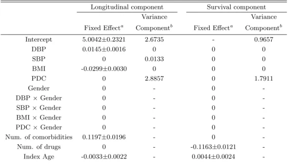
2.4 Data Application

To illustrate the method, I analyzed observational data from the CHF study. As previously stated, the main purpose of the investigation is to assess the effects of medication adherence on disease exacerbation and patient survival. For the survival outcome, I modeled the time from the first recorded CHF diagnosis to patient mortality, which could be censored on Dec 31, 2009. For the longitudinal outcome, I modeled the repeatedly measured BNP levels as markers of disease exacerbation. Because the distribution of BNP skewed strongly to the right, I used the logarithmic-transformed BNP (log(BNP)) in the model. Medication adherence, the independent variable of primary interest, was the average proportion of days covered (PDC) by all prescribed medications within each patient (Choudhry et al., 2009). Besides PDC, seven other risk factors were considered, including systolic blood pressure (SBP), diastolic blood pressure (DBP), BMI, gender, age at CHF diagnosis date (IndexAge), number of comorbidities (NumComorbid) and number of medications taken (NumMed). I also considered interactions among SBP, DBP, BMI, PDC and gender.

In the study sample, 58.3% of the subjects were females and the average BMI was 32.7

(kg/m2). The average age for the study cohort at the CHF diagnosis date was 62.7 years.

On average, the study subjects had 5.1 comorbidities and took 8.4 medications with a mean PDC of 0.327. Among the covariates, concurrently measured SBP (mean: 134.8mmHg; SD: 24.2 mmHg) and DBP (mean: 77.0mmHg; SD: 16.0 mmHg) were recorded at the time of BNP assessment; the remaining variables were collected as baseline covariates. The

censoring percentage was 64.1%, and median time to death was 4115 days (11.3 years).

For longitudinally measured BNP levels, I use linear mixed-effects model log(BN P)ij =

x1,ijβ1+z1,ijΓ1bi+εij fori= 1, ...,1702, andj = 1, ..., ni. I let x1,ij = (1, DBPij, SBPij, BM Ii, P DCi, Genderi, DBPij × Genderi, SBPij ×Genderi, BM Ii ×Genderi, P DCi × Genderi,N umComorbidi, N umM edi, IndexAgei) be the design matrix of the fixed effects

(50)

and z1,ij = (1, DBPij, SBPij, BM Ii, P DCi) be the design matrix of the random effects. I

assume thatbi follows N(0,I5) and I let εij ∼i.i.d.N(0, σ2) be the measurement error.

For mortality, I assume that the survival time ti follows a Weibull distribution. I use

a proportional hazard model h(ti) = h0(ti) exp(x2,iβ2 +z2,iΓ2bi), with baseline hazard

h0(ti) =αλtiα−1 for i= 1, ...,1702, where α is the shape parameter and λ is the scale

pa-rameter. I letx2,i= (1, DBPi1, SBPi1, BM Ii, P DCi, Genderi, DBPi1×Genderi, SBPi1×

Genderi, BM Ii ×Genderi, P DCi ×Genderi, N umComorbidi, N umM edi, IndexAgei) be

the design matrix for the fixed effects and z2,i = (1, DBPi1, SBPi1, BM Ii, P DCi) be the

design matrix for the random effects. Given the random effectbi, I assume that log(BN P)ij,

log(BN P)ij0 and t_i are conditionally independent.

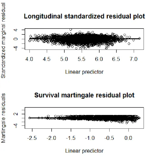
Data analytical results are presented in Table 2.11. For longitudinally measured BNP, our procedure selects DBP, BMI, NumComorbid, and IndexAge as non-zero fixed effects; SBP and PDC as non-zero random effects. For the survival outcome, NumMed is selected as the non-zero fixed effect; PDC as non-zero random effect. The residual plots Figure 2.1 show no violation of basic model assumptions for the two outcomes. The selected model has a smaller BIC value than the full model and a reduced model including all fixed effects and random intercept.

The effects of the selected variables on the outcomes are in expected directions. In the

longitudinal model, DBP is positively associated with BNP (β = 0.0145) (greater diastolic

dysfunction is associated with increased BNP level). BMI exhibits a significant negative association with BNP. For each unit of increase in BMI, log-BNP level decreases by 0.0299

(β =−0.0299). This result is not surprising as patients at advanced stage of CHF (indicated

by greater BNP values) tend to have deteriorated health and much reduced body weight. Interestingly, blood pressure is not found to be associated with the survival outcome, which is influenced more strongly by the number of medications. Patients taking more