7-6-2012
An efficient method of estimation for longitudinal
surveys with monotone missing data
Ming Zhou
Iowa State UniversityJae Kwang Kim
Iowa State University, [email protected]
Follow this and additional works at:
http://lib.dr.iastate.edu/stat_las_pubs
Part of the
Design of Experiments and Sample Surveys Commons,
Longitudinal Data Analysis
and Time Series Commons, and the
Statistical Methodology Commons
The complete bibliographic information for this item can be found at
http://lib.dr.iastate.edu/
stat_las_pubs/106. For information on how to cite this item, please visit
http://lib.dr.iastate.edu/
howtocite.html.
This Article is brought to you for free and open access by the Statistics at Iowa State University Digital Repository. It has been accepted for inclusion in Statistics Publications by an authorized administrator of Iowa State University Digital Repository. For more information, please contact
CHAPTER 5. AN EFFICIENT METHOD OF ESTIMATION FOR LONGITUDINAL SURVEYS WITH MONOTONE MISSING DATA
A paper to be submitted toBiometrika
Ming Zhou and Jae Kwang Kim
Department of Statistics & Statistical Laboratory Iowa State University
Ames, IA, 50011, USA
Abstract
Panel attrition is frequently encountered in panel sample surveys. When the panel attrition is related with the observed study variable observed in the previous years, the classical approach of nonresponse adjustment using a covariate-dependent dropout mechanism can be biased. We consider an efficient method of estimation with monotone panel attrition when the response probability depends on the previous values of study variable as well as other covariates. The proposed estimator is asymptotically optimal in the sense that it minimizes the asymptotic variance of a class of estimators that can be written as a linear combination of the unbiased estimators of the panel estimates for each wave. The proposed estimator incorporates all available information using the idea of generalized method of moments. Variance estimation is discussed and results from two limited simulation studies are also presented.
Key Words: Ignorable Missing; Generalized Method of Moments; Panel attrition; Survey in Time, Survey Sampling.
5.1 Introduction
Longitudinal surveys or panel surveys, surveys in which similar measurements are made on the same sample at different points in time, are very popular in the study of social and physical dynamics that cannot be inferred from cross-sectional surveys. Missing data in the response variable is a serious impediment to performing a valid statistical analysis in longitudinal surveys, and estimation with longitudinal missing data is quite challenging. Bollinger and David(1997,
2001), for example, used the Survey of Income and Program Participation (SIPP) data to show that estimates of food-stamp participation adjusted for nonresponse are significantly different from estimates that fail to account for nonresponse. Wun et al.(2007) andHawkes and Plewis
(2006) showed empirically that modeling the response probability is important for reducing the bias in the estimates.
A popular practice for nonresponse adjustment for panel survey assumes that the implicit response mechanism is the covariate-dependent missing, as termed byLittle (1995), where the response probability depends on the base-year covariate Xi that does not change over time,
but not on the study variable Yit that may vary over time. The nonresponse mechanism is
called ignorable if the true response probability depends only on the observed data and does not depend on unobserved random variables. In a panel survey, ignorable response mechanism means that the response probability at time t may depend on Xi and Yis with s < t, but
not on Yit. The covariate-dependent missing mechanism can be quite restrictive because the
dropout mechanism may not be fully explained by demographic base year covariates. For example, Korinek et al. (2007) analyzed the Current Population Survey (CPS) data using an area level model of response rate on average income and found that the response probability is strongly correlated with household income. They went on further concluding that the current adjustment method, which is essentially based on the covariate-dependent missing assumption, should be rejected.
Robins et al. (1995) have developed a method for the estimation of longitudinal regression models under ignorable nonresponse. Robins et al. (1995) assumed a working outcome regres-sion model for Yit, as well as the response propensity model for the response probability, in
developing their estimator. Rotnitzky et al.(1998) extended the method ofRobins et al.(1995) to nonignorable missingness. However, the Robins et al.(1995) method does not make full use of available information.
Under the response model of Robins et al. (1995), we consider an alternative method of parameter estimation that uses all available information in the longitudinal data. The basic idea for combining all available information is based on the generalized method of moments (GMM) estimation procedure of Hansen (1982). For T=1, the proposed estimator reduces to the optimal estimator considered in Cao et al. (2009). Thus, the proposed estimator is a generalized version of the existing optimal estimator for longitudinal surveys. By the orthogonal construction of the control variates, the computation of the optimal estimator is simplified.
In Section5.2, basic setup is introduced. In Section5.3, optimal propensity score estimator is motivated under the GMM framework. In Section 5.4, the optimal estimator under the panel survey setup is proposed. In Section 5.5, the proposed method is extended to complex survey sampling. In Section5.6, results from two limited simulation studies are presented and concluding remarks are made in Section 5.7.
5.2 Basic Setup
Let Yit(i = 1, . . . , n, t = 0, . . . , T) be the outcome of interest measured on the ith
sub-ject at year t, Xi be the corresponding auxiliary information that is always observed and
remains constant throughout different years. We use rit to denote the indicator of response
for subject i at year t: rit = 1 if Yit is observed and rit = 0 otherwise. We shall regard
(Xi, ri0, ri1, . . . , riT, Yi0, . . . YiT), i = 1, . . . , n, as independent and identically distributed
ran-dom vectors. Assume that the baseline information for subject i, (Xi, Yi0), is always
ob-served. Our goal is to estimate µt = E(Yit), the mean of Yit, for t = 1, . . . , T. Denote
Li,t = (Xi0, Yi0, Yi1, . . . , Yi,t)0 be the observed values of (X, Y) for uniti up to time t. For any
random variable ∆, we use ˜E to denote the sample average of ∆, that is ˜ E{∆}=n−1 n X i=1 ∆i. (5.1)
If the sample is obtained from a complex sampling design, ˜E{∆} represent a design-unbiased estimator of E{∆} based on the theory ofHorvitz and Thompson (1952).
Throughout this paper, we shall assume that the missing pattern is monotone, that is,
ri,j = 0⇒ri,j+1 = 0,∀j = 1, . . . , T −1. (5.2)
Although the constraint (5.2) can be somewhat restrictive, we believe that the monotone miss-ing will cover most realistic situations for the panel attrition. The extension to non-monotone missing pattern is beyond the scope of this paper. We shall assume the following missing data mechanism:
P r(rit= 1|ri,t−1 = 1, Li,T) =P r(ri,t = 1|ri,t−1 = 1, Li,t−1). (5.3)
Equation (5.3) means that the data are “missing at random” in the sense ofRubin(1976). See also Little(1995) for its meaning under longitudinal survey setup. Equation (5.3) means that, at any yeart, the probability thatYit is missing only depends on what is observed by timet−1.
In other words, among subjects observed at timet−1, the nonresponse probability at timetis unrelated to the current and future outcomesYit, . . . , YiT. The missing data mechanism in (5.3)
is more realistic than the covariate-dependent missing mechanism, which is often assumed in the usual nonresponse adjustment methods that use the demographic variables as the covariates for the nonresponse model. In addition to (5.3), we assume that
pit:=P(rit = 1|ri,t−1 = 1, Li,t−1)> σ >0, t= 1, . . . , T, (5.4)
so that for each subjecti, the probability of remaining in the study is bounded away from zero, which is needed to guarantee the existence of n1/2-consistent estimators of µ
t (Robins et al.,
1994). The probabilitypit is the conditional probability of response at time tgiven the unit i
response at timet−1. Assumptions (5.2) and (5.3) imply that
πit:=P(rit= 1|Li,T) =P(rit= 1|Li,t−1) =P(ri0= 1)
t
Y
j=1
pij. (5.5)
The response probabilityπitis also often called propensity score (Rosenbaum and Rubin,1983).
is under control of the investigator. The probabilityπitis different frompitin thatπitrefers to,
for subject i, the marginal probability of response at timet, while pit refers to the conditional
probability of a response at time t given that unit i responds at time t−1. Very often πit
depends onLi,t−1 and the average of the observed Yit’s,
ˆ µt,naive= P iritYit P irit , (5.6)
will in general be inconsistent forµt. In this case, a commonly adopted approach is to model
the response probability and use the estimated response probability to obtain the propensity score adjusted (PS) estimators. We discuss the PS estimator in more detail in the upcoming section.
5.3 Optimal PS Estimation
5.3.1 PS Estimation
For simplicity, let us start from theT = 1 case. We now absorbYi0intoXi, and denote it as
Xi solely. The outcome of interest is thenYi1 and we are interested in estimatingµ1=E(Yi1).
Let the true response probability be parametrically modeled by πi1 = π1(Xi;φ1), for some
functionπ1(.) known up to φ1. If the maximum likelihood estimator ofφ1, the solution to
S1(φ1) = ˜E (r1−π1) ∂π1/∂φ1 π1(1−π1) = 0, (5.7)
denoted by ˆφ1, is available, then the propensity score adjusted (PS) estimator ofµY1, denoted
by ˆµY1,P S, can be computed by solving
ˆ U1,P S := ˜E r1 ˆ π1 (Y1−µ1) = 0, (5.8)
for µ1. Inverse probability weighted estimating equations have been previously considered by
Horvitz and Thompson (1952), Manski and Lerman (1977), Flanders and Greenland (1991),
Robins et al. (1995) among others. Strictly speaking, the PS estimator in (5.8) is also a function of ˆφ1. To discuss the asymptotic variance of the PS estimator, we introduce the
Lemma 5.1. Suppose z1, . . . , zn are independent and identically distributed random vectors
and ˆγ is the solution to E˜{U(z;γ)} = 0. Let Ui(γ) = U(zi;γ). If (i) E{U(γ∗)} = 0 and
ˆ
γ =γ∗+op(1), where γ∗ is an interior point of the parameter space; (ii) V ar{U(γ∗)}is finite;
(iii) U(γ) is continuously differentiable in a neighborhoodN of γ∗; (iv) E{∂U(γ∗)/∂γ} exists
and is nonsingular; (v)E
supγ∈Nk∂U(γ)/∂γk <∞. Then, ˆ γ−γ∗ = − E ∂U(γ∗) ∂γ −1 ˜ E{U(γ∗)}+op(n−1/2). (5.9)
Proof. This lemma is an immediate application of Lemma 2.4 and Theorem 3.1 ofNewey and
McFadden (1994).
Remark 5.1. Consider Ui(γ) = (θ0 −gi(φ)0, ψi(φ)0)0, where γ = (θ0, φ0)0, S(φ) = Piψi(φ) is
the score function for φ. Let ˆγ be the solution to ˜E{U(γ)} = 0, that is, ˆγ = (ˆθ0,φˆ0)0, where ˆ
θ= ˜E{g( ˆφ)}. Assume that conditions in Lemma 5.1are satisfied. Then (5.9) reduces to
ˆ θ−θ∗ ˆ φ−φ∗ = − I −E{∂g(φ∗)/∂φ} 0 E{∂ψ(φ∗)/∂φ} −1 ˜ E{g(φ∗)} ˜ E{ψ(φ∗)} +op(n −1/2). (5.10)
By differentiating E{g(φ)} with respect to φunder the integral sign and evaluating at φ∗, we obtain −E{∂g(φ∗)/∂φ}= E{g(φ∗)ψ(φ∗)}=Cov{g(φ∗), ψ(φ∗)}, similarly −E{∂ψ(φ∗)/∂φ} =
E{ψ(φ∗)ψ(φ∗)0}=V ar{ψ(φ∗)}(Pierce,1982) . Therefore, ˆθcan be expressed as ˆ
θ−θ∗ = ˜E{g(φ∗)} −Cov{g(φ∗), ψ(φ∗)}[V ar{ψ(φ∗)}]−1E˜{ψ(φ∗)}+op(n−1/2). (5.11)
This implies that
V ar[ ˜E{g( ˆφ)}] =V ar[ ˜E{g(φ∗)}|S⊥] +o(n−1), (5.12) where V ar{E˜{g( ˆφ)|S⊥}:=V ar[ ˜E{g(φ∗)}] −Cov[ ˜E{g(φ∗)}, S(φ∗)][V ar{S(φ∗)}]−1Cov[S(φ∗),E˜{g(φ∗)}]. (5.13) Note that by (5.12), V ar ˜ E r1Y1 ˆ π1 ≈V ar ˜ E r1Y1 π1 S1⊥ ≤V ar ˜ E r1Y1 π1 .
Such contradictory phenomena has been discussed byRosenbaum(1987),Robins et al.(1994),
Little and Vartivarian (2005), Kim and Kim (2007), Beaumont and Bocci (2009). See also
Henmi and Eguchi(2004).
5.3.2 Optimal PS Estimation
We now discuss optimal PS estimation. We assume that the propensity score is computed as in (5.7). In general, the PS estimator ˆµX,P S applied to µX = E(X) is not equal to the
complete sample estimator ˆµX,n = ˜E{X}. Thus, the complete sample estimator ¯Xn can be
used to improve the efficiency of the PS estimator. To combine all the available information, we consider minimizing the following objective function
Q= ˆ X1−µX ˆ X2−µX ˆ Y1−µ1 0 V ar ˆ X1 ˆ X2 ˆ Y1 −1 ˆ X1−µX ˆ X2−µX ˆ Y1−µ1 , (5.14)
with respect to µX and µ1, where ˆX1 and ˆX2 are two unbiased estimators of µX and ˆY1 is
an unbiased estimator of µ1. The estimator obtained from the minimization of Q in (5.14) is
often called the GMM, termed by Hansen (1982), and is very popular in econometrics. The GMM setup provides a useful tool for combining information from different sources. Under the missing data setup where Xi is always observed andYi1 is subject to missingness, if we know
πi1, then we can evaluate ˆX1 = ˜E{X},Xˆ2 = ˜E{r1X/π1},Yˆ1 = ˜E{r1Y1/π1}. In this case, the
optimal estimator that minimizes (5.14) is obtained by ˆ µ1 = ˜E r1Y1/π1−(r1/π1−1)X0B∗ , where B∗ =EhE˜{(1/π1−1)XX0} i−1 EhE˜{(1/π1−1)XY1} i .
In practice, we can estimate B∗ by the plug-in estimator ˆ µ1,opt= ˜E n r1Y1/π1−(r1/π1−1)X0Bˆ∗ o , (5.15) where ˆ B∗ = ˜E r1 π1 (1/π1−1)XX0 −1 ˜ E r1 π1 (1/π1−1)XY1
The estimator (5.15) is an (asymptotically) optimal estimator among the class of linear unbiased estimators. A PS estimator is said to have external consistency if it is equal to the full sample estimator ˜E{Y1} when Yi1 = Xi0β for some β for all i. Note that the optimal
estimator (5.15) satisfies a calibration constraint in the sense that, if Yi1 = Xi0β for some β
for all i, then ˆB∗ = β, and ˆµ1,opt = ˜E{r1(Y1−Y1)/π1+Y1} = ˜E(Y1). Thus, the direct PS
estimator ˆY1,P S is not externally consistent but the optimal estimator in (5.15) is.
If the true propensity scores are unknown, we will use ˆX1 = ˜E{X}, ˆX2 = XˆP S =
˜
E{r1X/πˆ1}, ˆY1 = ˆY1,P S = ˜E{r1Y1/πˆ1}, where ˆπ1 = π1(X; ˆφ1), with ˆφ1 being the maximum
likelihood estimator given by (5.7). In this case, the optimal estimator of µX is still equal to
˜
E{X}, but the optimal estimator of ˆµ1,optin (5.15) using ˆπi1instead ofπi1 is not really optimal
because the covariance between ˆY1,P S and ( ˆXP S,Xˆn) is different from the covariance between
˜
E{r1Y1/π1} and ( ˜E{r1X/π1},Xˆn). To construct an optimal estimator, we can consider an
estimator of the form
ˆ
µ1,B = ˆY1,P S−( ˆXP S−Xˆn)B
indexed byB and findB∗ that minimizes the variance of ˆµ1,B. The solution is
B∗ =nV ar( ˆXP S−Xˆn) o−1 Cov( ˆXP S−Xˆn,Yˆ1,P S). By (5.12), we can approximateB∗ by B∗ = h V ar{E˜(r1X/π1)−Xˆn|S⊥1} i−1 Cov{E˜(r1X/π1)−Xˆn,E˜(r1Y1/π1)|S1⊥}. (5.16)
Thus, the optimal estimator in (5.14) with ˆX1 = ˆXn,Xˆ2 = ˆXP S,Yˆ1 = ˆY1,P S can be obtained
by minimizing
Q= ( ˆZ−µZ)0{V ar( ˆZ0|S1⊥)}−1( ˆZ−µZ), (5.17)
where ˆZ = ( ˆXn,XˆP S,Yˆ1,P S)0,Zˆ0 = ( ˆXn,E˜{r1X/π1},E˜{r1Y1/π1}) and µZ = (µX, µX, µY1).
The optimalQterm in (5.17) can be also obtained by minimizing the augmentedQterm given by Q∗ = ˆ Z−µZ S1 0 V ar ˆ Z0 S1 −1 ˆ Z−µZ S1 , (5.18)
where S1(φ1) is the score function of φ1, defined in (5.7). To see this, note that Q∗ can be
decomposed into
Q∗ ={Zˆ−µZ−V ar( ˆZ0)−1Cov( ˆZ0, S1)S1}0{V ar( ˆZ0|S1⊥)}−1 × {Zˆ−µZ−V ar( ˆZ0)−1Cov( ˆZ0, S1)S1}+S10V ar(S1)−1S1
=Q+S10V ar(S1)−1S1,
where Q is defined in (5.17). Because S10V ar(S1)−1S1 does not involve µZ, the optimal
esti-mator of µZ can be also be computed by minimizing Q∗ term in (5.18). Thus, the effect of
using the estimated propensity score can be easily taken into account by simply adding the score function for φ1 into theQ term. Furthermore, as shall be discussed in Theorem5.2, the
inclusion of the score function into the GMM makes the linearization for variance estimation easy. The following example gives an explicit formula for the optimal PS estimator whenφ1 is
estimated by its maximum likelihood estimator.
Example 5.1. Under the response model where the score function forφ1 is
S1(φ1) = ˜E r1 π1(φ1) −1 h(φ1) ,
The coefficientB∗ corresponding to the optimal PS estimators in the family ˆ µ1,B = ˆY1,P S−( ˆXP S−Xˆn)0B, is given by B∗ ={VXX−VXSVSS−1VSX}−1{VXY −VXSVSS−1VSY}, where VXX VXY VXS VY X VY Y VY S VSX VSY VSS =V ar ˜ E{(r1/π1−1)X} ˜ E{r1Y1/π1} ˜ E{(r1/π1−1)h} .
Thus, a consistent estimator ofB∗ is given by
ˆ B∗ = (Ip, O) ˜ E r1 ˆ π1 1 ˆ π1 −1 X h(X) X h(X) 0 −1 ˜ E r1 ˆ π1 1 ˆ π1 −1 X h(X) Y1 , (5.19)
wherep=dim(X), and the resulting optimal estimator is ˆ
Y1,opt= ˆY1,P S −( ˆXP S−Xˆn)0Bˆ∗. (5.20)
The estimator in (5.20) is equal to the optimal estimator presented inCao et al. (2009) in the context of a doubly robust estimator. Similar but slightly different approach was proposed by Tan (2006). However, our derivation of the optimal estimator in (5.20) is different from those ofCao et al.(2009) andTan(2006). In addition, the GMM setup used in deriving (5.20) can be easily generalized in longitudinal missing data, which will be discussed in the following section.
5.4 Proposed Method for Longitudinal Missing
The proposed optimal estimator in Section 5.3 is based on the GMM setup and it can be easily extended to the problem of optimal estimation with longitudinal missing. To correctly account for the ignorable dropout mechanism in (5.3), we shall assume a parametric model for pit, given by pit(Li−1;φt). Note that we do not make any explicit assumptions for the
marginal distribution of Li,T, we only use the response model, which is attractive in handling
unit nonresponse in sample surveys. The partial likelihood regarding φt’s is then
L(φ1, . . . , φT) = n Y i=1 T Y t=1 pri,t it (1−pit)1−ri,t ri,t−1 . (5.21)
The corresponding score function is then ¯ ST := (S1(φ1), . . . , ST(φT))0 = ∂logL(φ1, . . . , φT) ∂φ1 , . . . ,∂logL(φ1, . . . , φT) ∂φT , (5.22) where St(φt) =nE˜ rt−1(rt−pt) ∂pt/∂φt pt(1−pt) (5.23) is the score function associated with the conditional response probability. A commonly adopted parametric model forpt is the logistic regression model
pt=
1
1 + exp{−φ0tLt−1}
Under this logistic regression model (5.24), the score function in (5.23) reduces to
St(φt) =nE˜{rt−1(rt−pt)Lt−1}. (5.25)
At each yeart, we can obtain PS estimators forµX, µ1, . . . , µt, using ˆπt. Thus, we have T+ 1
estimators of µX and T −t+ 1 estimators of µt computed by the inverse probability weights
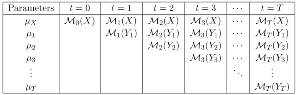
at yearst, . . . , T. To illustrate it, denote operator Mt as
Mt(∆) = ˜E rt∆ ˆ πt , t= 0,1, . . . . (5.26)
Then we can obtain a collection of PS estimators forLT, as shown in Table5.1. In yeart= 2,
for example, M2(X) is available for µX, M2(Y1) is available for µ1, and M2(Y2) is available
forµ2.
Table 5.1 List of available unbiased estimators of the parameters for each year Parameters t= 0 t= 1 t= 2 t= 3 · · · t=T µX M0(X) M1(X) M2(X) M3(X) · · · MT(X) µ1 M1(Y1) M2(Y1) M3(Y1) · · · MT(Y1) µ2 M2(Y2) M3(Y2) · · · MT(Y2) µ3 M3(Y3) · · · MT(Y3) .. . . .. ... µT MT(YT)
To incorporate all available information, we use adopt GMM method in Section5.3. Denote
ut=rt/pt−1, t= 1, . . . , T, and ψt−1= r0u1p1L0 r1u2p2L1 .. . rt−1utptLt−1 , (5.27)
where L0 = (X0, Y0)0 and Lj = (X0, Y0, Y1, . . . , Yj)0 for j = 1, . . . , t −1. Note that at
each year t, E(rt−1utptLt−1) = 0, because E(rt−1utptLt−1|Lt−1, r1 = . . . = rt−1 = 1) =
to construct PS estimators for µX, µY1, . . . , µt using ˜E(rtX/πt), ˜E(rtY1/πt), . . ., ˜E{rtYt/πt}
respectively. Similar to the t= 1 case, at year t, we get the following control variates
ξt−1 = r0 π0u1L0 r1 π1u2L1 .. . rt−1 πt−1utLt−1 . (5.28)
By the definition of the response probabilities, we have rt−1ut/πt−1 =rt/πt−rt−1/πt−1 and
E{ξt−1}= 0. Therefore, we propose the following optimal estimator forE(Yt) as the minimizer
to the following quadraticQt, with respect toµt, using the fact thatE{ψt−1}= 0, E{ξt−1}= 0,
Qt= ˜ E{rtYt/πˆt} −µt ˜ E{ξˆt−1} ˜ E{ψt−1} 0 ˆ V ar ˜ E{rtYt/πt} ˜ E{ξt−1} ˜ E{ψt−1} −1 ˜ E{rtYt/πˆt} −µt ˜ E{ξˆt−1} ˜ E{ψt−1} , (5.29)
where ˆξt−1 isξt−1after plugging in the maximum likelihood estimator ˆφ1, . . . ,φˆtgiven by (5.22).
The control variate ˆξt−1is included to incorporate all available information up to yeart−1 and
the control variate ˜E(ψt−1) is included to incorporate the score equation for (φ01, . . . , φ0t−1)0.
Fort= 1, ˜E( ˆξ0) = ˆXP S−Xˆn and ˜E(ψt−1) =n−1S1. Note that we can write ¯ST =nE˜{ψT−1}.
For example, when T = 3,
ξ2= r0 π0u1L0 r1 π1u2L1 r2 π2u3L2 , ψ2 = (r1−p1r0)L0 (r2−p2r1)L1 (r3−p2r2)L2 .
Intuitively speaking, when estimatingE(Y3), we have four PS estimators forX, which are ˜E(X),
˜
E(r1X/ˆπ1), ˜E(r2X/πˆ2), ˜E(r3X/πˆ3); three PS estimators for Y1, i.e., ˜E(r1Y1/πˆ1), ˜E(r2Y2/ˆπ2),
˜
E(r3Y1/πˆ3); two PS estimators forY2, ˜E(r2Y2/πˆ2),E˜(r3Y2/πˆ2). Those nine PS estimators
pro-duce six atomic control variates represented by ˆξ2, in the sense that any difference between
two PS estimators for estimating the same mean, say ˜E(rjz/πˆj)−E˜(riz/πˆi), can be written
as a linear combination of ˜E{ξˆ2}, wherez can be any past information before yeart. Formally
speaking, the following theorem gives our optimal PS estimator for µt for t= 1, . . . , T. Note
are also orthogonal and ˆV{E˜(ξt−1)} and ˆV{E˜(ψt−1)} are block diagonal matrices. This
or-thogonality of the control variates makes the computation of the resulting optimal estimator simple.
Theorem 5.1. Under the regularity conditions given in Appendix5.A.1and the response model (5.24) such that the score equation for (φ01, . . . , φ0T)0 is E˜(ψT−1) = 0, for each year t, the
coefficient Bt∗ corresponding to the optimal estimator of µt=E{Yt} among the class
˜ E(rtYt/πˆt)−B0tE˜( ˆξt−1), is given by Bt∗= (B1∗t0, . . . , Btt∗0)0, where B∗jt= (Idim(Lj−1), O)E−1 rj−1 1 pj −1 1 πj−1Lj−1 pjLj−1 1 πj−1Lj−1 pjLj−1 0 ×E 1 pj −1 1 πi−1Li−1 piLi−1 rtYt πt . (5.30)
A consistent estimator for B∗jt is
ˆ Bj,t = (Idim(Lj−1), O) ˜E −1 rtπˆj−1 ˆ πt 1 ˆ pj −1 1 ˆ πj−1Lj−1 ˆ pjLj−1 1 ˆ πj−1Lj−1 ˆ pjLj−1 0 ×E˜ 1 ˆ pj −1 1 ˆ πi−1Li−1 ˆ piLi−1 rtYt ˆ πt . (5.31)
The resulting optimal estimator that minimizes (5.29) is ˆ Yt,opt = ˜E{rtYt/πˆt} − t X j=1 ˆ Bj,t0 E˜ rj−1uˆjLj−1 ˆ πj−1 , (5.32) where uˆj =rj/pˆj −1 and pˆj =pj(Lj−1; ˆφj).
Proof. See Appendix.
Remark 5.2. Fort= 1, r0≡1, π0 ≡1, the estimator is
˜ E{rˆ1Y1/πˆ1} −Bˆ10,1E˜ r0 π0 ˆ u1L0 = ˜E r1 ˆ p1 Y1−Bˆ10,1 r1 ˆ p1 −1 X ,
where ˆ B1,1 = (I, O) ˜ E r1 ˆ p1 1 ˆ p1 −1 X ˆ p1X X ˆ p1X 0 −1 ˜ E r1 ˆ p1 1 ˆ p1 −1 X ˆ p1X Y1 ,
which is the same estimator as given in Example5.1.
We now discuss variance estimation of the optimal estimator in (5.32). Strictly speaking, ˆ
Yt,opt is a function of ( ˆφ1, . . . ,φˆt) and should then be written as ˆYt,opt( ˆφ1, . . . ,φˆt). We show in
Theorem5.2that we can safely ignore the effects of ˆφ1, . . . ,φˆtin ˆYt,optfor linearization variance
estimation. That is, ˆYt,opt( ˆφ1, . . . ,φˆt) = ˆYt,opt(φ∗1, . . . , φ∗t) +op(n−1/2), which is often referred
to asRandles(1982) condition. SeeKim and Rao(2009), for details.
Theorem 5.2. Under the regularity conditions in Appendix 5.A.1, Yˆt,opt in (5.32) is
asymp-totically linear with influence function ηt, where
ηt= rtYt πt − t X j=1 Dj,t0 rt−1ut 1 πj−1Lj−1 pjLj−1 , (5.33) where Dj,t=E−1 rj−1 1 pj −1 1 πj−1Lj−1 pjLj−1 1 πj−1Lj−1 pjLj−1 0 E 1 pj −1 1 πj−1Lj−1 pjLj−1 rtYt πt . Thus, √ n( ˆYt,opt−µt) d − →N{0, V ar(ηt)} (5.34) and also ˆ V−1/2( ˆYt,opt−µt) d − →N(0,1), (5.35) where ˆ V =n−1(n−1)−1E˜{ηˆt−E˜(ˆηt)}2, (5.36)
and ηˆt is ηt with the estimated parameters plugged-in.
Remark 5.3. We obtain ˆµt,opt by minimizingQtin (5.29) with respect toµt. One may consider
estimatingµ1, . . . , µT simultaneously by minimizing the following term
˜ QT = ˜ E{X} −µX ˜ E{r1Y1/ˆπ1} −µ1 .. . ˜ E{rTYT/πˆT} −µT ˜ E{ξˆT−1} −E{ξT−1} ˜ E{ψT−1} −E{ψT−1} 0 ˆ V ar ˜ E{X} ˜ E{r1Y1/π1} .. . ˜ E{rTYt/πT} ˜ E{ξT−1} ˜ E{ψT−1} −1 ˜ E{X} −µX ˜ E{r1Y1/πˆ1} −µ1 .. . ˜ E{rTYT/πˆT} −µT ˜ E{ξˆT−1} −E{ξT−1} ˜ E{ψT−1} −E{ψT−1} , (5.37) with respect to (µ0X, µ1, . . . , µT)0. It can be shown that under monotone missing pattern,
minimizing ˜QT to estimateµ1, . . . , µT simultaneously is equivalent to minimizing ˜QT in (5.37)
for each µt (see Appendix). The dimension of the vector in (5.37) is 2qT +T2+ 1, while the
dimension associated with Qt in (5.29) is 2qt+t2−t+ 1, whereq =dim(X).
5.5 Extension to Complex Survey Sampling
In this section, we extend the result to complex survey sampling by considering a fi-nite population indexed by UN = {1,2, . . . , N} with known population size N. Let FN =
{(Xi0, Yi1, . . . , YiT)0 | i = 1, . . . , N}. At each time t, Yit is subject to missingness indicated
by rit, which takes the value 1 if unit i is responding and takes the value 0 otherwise. We
shall assume monotone missing pattern as described in (5.2), and adopt missing at random mechanism as in (5.3). LetA denote the set of indices for the subjects in a sample selected by a probability sampling, with fixed sample size nand design weights ωi, i= 1, . . . , N. Assume
that the sampling indicatorsI{i∈A}, i= 1, . . . , N, are independent of missing indicators rit.
We use notations ˜E,E˜A defined as
˜ E{∆}=N−1 N X i=1 ∆i, E˜A{∆}=N−1 X i∈A ωi∆i. (5.38)
points, µt= ˜E{Yt}=N−1 N X i=1 Yit, t= 1, . . . , T. (5.39)
Under logistic regression model in (5.24), the score function for estimating φtis
St(φt) = ˜EA{rt−1(rt−pt)Lt−1/w}=
X
i∈A
ri,t−1(ri,t−pi,t)Li,t−1. (5.40)
The PS estimator forµt in (5.39) then is
ˆ Yt,P S = ˜EA rtYt ˆ πt = 1 N X i∈A ωi ritYit ˆ πit . (5.41)
To apply the GMM methodology, we shall adopt ξt−1 in (5.28), ψt−1 in (5.27), and
con-struct a Qt term similar to (5.29). Note that E{E˜A(rtYt/πt)|FN} = ˜E(rtYt/πt) = µt. Since
E[I{i ∈ A}ri,t−1(rit/pit−1)|FN] = E[I{i ∈ A}|FN]·E{ri,t−1(ri,t −pit)|FN} = 0, we have
E{EA(ξt−1)|FN}= 0, andE{E˜A(ψt−1/w)|FN}= 0. Thus we can consider theQtterm similar
to (5.29) as Qt= ˜ EA{rtYt/ˆπt} −µt ˜ EA{ξˆt−1} ˜ EA{ψt−1/w} 0 ˆ V ar−1 ˜ EA{rtYt/πt} ˜ EA{ξt−1} ˜ EA{ψt−1/w} FN ˜ EA{rtYt/ˆπt} −µt ˜ EA{ξˆt−1} ˜ EA{ψt−1/w} . (5.42)
The details of the key steps for deriving the optimal solution to minimizeQtin (5.42) are given
in the Appendix. To discuss the asymptotic properties of the PS estimators in the complex survey, the following conditions are assumed in addition to the regularity conditions (C1)-(C6) stated for Theorem5.1.
(C7) The design weight is bounded from above and below, that is, 0< Kl≤nN−1ωi ≤Ku <∞,
for all i= 1, . . . , N, uniformly inn, whereKl and Ku are fixed constants.
(C8) The sample moments with design weight converges to the population moments, that is, 1 N X i∈A ωiuiu0i = 1 N N X i=1 uiu0i+op(1),
Corollary 5.1. Let FN ={(Xi0, Yi,1, . . . , Yi,T)0 |i= 1, . . . N} be a finite population subject to
missingness at t= 1, . . . , T. A sample of size n is selected using design weights ωi. Subject to
conditions (C1) - (C8), under monotone missing pattern and response model in (5.24) such that the score equation for (φ01, . . . , φ0T)0 is NE˜{ψT−1} = 0, the optimal estimator ofµt among the
class E˜A{rtYt/ˆπt} −Bt0E˜A{ψˆt−1} is E˜A{rtYt/πˆt} −Bt∗0E˜A{ψˆt−1}, where Bt∗= (B∗1t 0, . . . , B∗ tt0)0 and Bjt∗ = (Idim(Lj−1),0) ˜ E wπj−1 1 pj −1 1 πj−1Lj−1 pjLj−1/w 1 πj−1Lj−1 pjLj−1/w 0 −1 ×E˜ w 1 pj −1 1 πj−1Lj−1 pjLj−1/w Yt , (5.43)
which can be consistently estimated by
ˆ Bj,t = (Idim(Lj−1),0) ˜ EA wrt ˆ πt ˆ πj−1 1 ˆ pj −1 1 ˆ πj−1Lj−1 ˆ pjLj−1/w 1 ˆ πj−1Lj−1 ˆ pjLj−1/w 0 −1 ×E˜A wrt ˆ πt 1 ˆ pj −1 1 ˆ πj−1Lj−1 ˆ pjLj−1/w Yt , (5.44)
The resulting optimal estimator for minimizing (5.42) is ˆ Yt,opt = ˜EA{rtYt/πˆt} − t X j=1 ˆ Bj,t0 E˜A rj−1uˆjLj−1 ˆ πj−1 , (5.45)
where uˆij =rij/pˆij −1, πˆij =Qkj=1pˆik and pˆij =pj(Li,j−1; ˆφj).
Remark 5.4. Whent= 1, note that we assume no missing in the baseline year, i.e. π0 = 1, the
optimal estimator for N−1PN
i=1Yi1 is ˆ Y1,opt= ˜EA{r1Y1/πˆ1} −Bˆ110 E˜A{(r1/πˆ1−1)X} =N−1X i∈A ωi ri1Yi1 ˆ πi1 −N−1X i∈A ωi ri1 ˆ πi1 −1 X0Bˆ11, where ˆB11 is (I, O) X i∈A ωi2ri1 ˆ πi1 1 ˆ pi1 −1 Xi ˆ pi1Xi wi Xi ˆ pi1Xi wi 0 −1 × X i∈A ωi2ri1 ˆ πi1 1 ˆ pi1 −1 Xi ˆ pi1Xi wi Yi1 .
Denote ηi,t= ritYit πit − t X j=1 Bj,t∗ 0ri,j−1ui,j Li,j−1 πi,j−1 − t X j=1 Cj,t∗ 0ri,j−1ui,j pi,jLi,j−1 wi , (5.46) where (Bj,t∗ 0, Cj,t∗ 0) =Dj,t∗ 0, and Djt∗ = ˜ E wπj−1 1 pj −1 1 πj−1Lj−1 pjLj−1/w 1 πj−1Lj−1 pjLj−1/w 0 −1 ×E˜ w 1 pj −1 1 πj−1Lj−1 pjLj−1/w Yt . (5.47) A consistent estimator ofDj,t is ˆ Dj,t= ˜ EA wrt ˆ πt ˆ πj−1 1 ˆ pj −1 1 ˆ πj−1Lj−1 ˆ pjLj−1/w 1 ˆ πj−1Lj−1 ˆ pjLj−1/w 0 −1 ×E˜A wrt ˆ πt 1 ˆ pj −1 1 ˆ πj−1Lj−1 ˆ pjLj−1/w Yt . (5.48)
Let ˆηi,t be the corresponding estimator of ηi,t in (5.46) with ˆDj,t,ˆπi,j,pˆi,j, then ˆYt,opt in (5.45)
can be written as ˆ Yt,opt= 1 N X i∈A ωiηˆi,t= 1 n X i∈A nωi N ηˆi,t.
By similar arguments in the proof of Theorem 5.2, ˜
EA(ˆηt) = ˜EA(ηt) +op(n−1/2),
and we can apply the standard complete sample method to estimate the variance of ˜EA(ηt),
which is asymptotically equivalent to the variance of ˜EA(ˆηt) (see Kim and Rao,2009).
To calculateV ar{E˜A(ηt)|FN}, thereverse framework ofFay(1992),Shao and Steel(1999),
Kim and Rao (2009) is used. Specifically, denote rt = {r11, . . . , rN t} and ¯rt = {r1, . . . ,rt}.
Then
V ar{E˜A(ηt)|FN}=V1+V2 =E[V ar{E˜A(ηt)|¯rt,FN}|FN] +V ar[E{E˜A(ηt)|¯rt,FN}|FN].
For any g with finite second moment, we assume that N−1P
i∈A
P
i∈AΩijgigj is a design
unbiased estimator of V ar{E˜(g)|FN}, where Ωij depends on the joint inclusion probability.
Then V ar{E˜A(ηt)|¯rt,FN} in (5.49) can be estimated by
ˆ V1(η) =N−2 X i∈A X j∈A Ωijηi,tηj,t.
To show the consistency of ˆV1 forV1 in (5.49), we assume that finite fourth moments exist for
variables stated in (C4), N X i=1 |ΩN.ij|=O(n−1N), (5.50) and V ar[nV ar{E˜A(ηt)|¯rt,FN}|FN] =op(1).
Consequently, ˆV1(η) is consistent forV1and ˆV1(ˆη) is also consistent forV1under same conditions
(see Kim et al., 2006). The second term V2 in (5.49) is V2 = V ar[E{E˜A(ηt)|¯rt,FN}|FN] =
V ar{E˜(ηt)|FN}. Note that E(ηt|FN) = E(rtYt/πt|FN) + 0 = Yt, rj−1uj/πj−1 = rj/πj − rj−1/πj−1, then ηt−E(ηt|FN) = rt πt −1 Yt− t X j=1 rj−1ujD∗j,t 0 Lj−1/πj−1 Lj−1pj/w = t X j=1 rj πj − rj−1 πj−1 Yt− t X j=1 rj−1ujD∗j,t 0 Lj−1/πj−1 Lj−1pj/w = t X j=1 rj−1uj Yt πj−1 − t X j=1 Dj,t∗ 0 Lj−1/πj−1 Lj−1pj/w .
Recall thatE(rj−1uj|FN) = 0, j = 1, . . . , T andE(ri−1uirj−1uj|FN) =πj−1(1/pj−1)I(i=j),
for any i, j. Then, the form ofV2 is
V2=N−2 N X i=1 t X j=1 1 πi,j−1 1 pij −1 Yit−πi,j−1 t X j=1 Dj,t∗ 0 Li,j−1/πi,j−1 Li,j−1pi,j/wi 2 , (5.51)
and it can be estimated by
ˆ V2 =N−2 X i∈A ωi t X j=1 1 ˆ πi,j−1 1 ˆ pij −1 Yit−πˆi,j−1 t X j=1 ˆ Dj,t0 Li,j−1/πˆi,j−1 Li,j−1pˆi,j/wi 2 . (5.52)
Under (C8), we have ˆV2 =V2+op(N−1). Therefore, ˆV{E˜A(ˆηt)}= ˆV1+ ˆV2 is consistent for the
variance ˆYt,opt in (5.45).
The order of the first term V1 is V1 = Op(n−1), while the order of the second term V2 is
V2 =Op(N−1). Thus, when the sampling fraction n/N is negligible, that is, n/N =o(1), the
second term V2 can be ignored, and ˆV1 would be a consistent estimator for the total variance.
5.6 Simulation Study
To test our theory and to examine the performance of the proposed estimator for finite sample sizes, we performed two simulation studies. In the first simulation study, we used a linear regression model with serial correlation. The model is
Y0 =X/2 +e0, Yt= 1 +X/2 +Yt−1+et,fort >1,
where X ∼ N(0,1), and et’s are independent and identically distributed as N(0,1). The
missing indicator rt follows the following distribution:
P(rt= 1|X, Yt−1, rt−1 = 1) = 1
1 + exp[−2.5−X+{Yt−1−(t−1)}/2]
,
and there are no missing data in the baseline year. In this simulation setup, the true mean of
Yt is E(Yt) = t. The parameters of interest are µt =E(Yt), for t= 1,2,3. We computed five
estimators for each parameter. The estimators include ˜E{Yt}, the full sample estimator under
no missingness; ˜E{rtYt}/E˜{rt}, the naive estimator using the simple mean of the responding
part of the sample; ˜E{rtYt/πˆt}, the direct PS estimator; ˆYt,opt, our optimal propensity score
adjusted estimator in (5.32). In addition, we considered an estimator from the class of estima-tors proposed byRobins et al.(1995) based on weighted estimating equations. Specifically, Let
ˆ Yt,RRZ be solution to ˜ E rt ˆ πt {Yt−µt−β10,t(X−E˜[X])} 1 X−E˜(X) = 0, (5.53) which gives ˆ Yt,RRZ = ˜ E{rtYt/πˆt} ˜ E{rt/ˆπt} −βˆ10,t E˜{rtYt/ˆπt} ˜ E{rt/πˆt} −X¯n ! . (5.54)
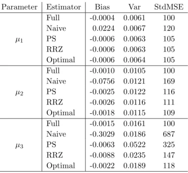
We usedB = 10,000 Monte Carlo samples of sizen= 500 for this simulation. The response rates for t = 1,2,3, are 0.90,0.83,0.76 respectively. The simulation results in Table 5.2 show that the naive estimator is severely biased as expected, and the other three PS estimators (direct, RRZ, optimal) are all nearly unbiased. The RRZ estimator is more efficient than the direct PS estimator because the regression model approximately holds. However, the RRZ estimator is less efficient than the optimal estimator.
We also computed a variance estimator of the optimal estimator using the formula in (5.36). The relative biases of the variance estimator in (5.36), for t = 1,2,3, are 0.0260, 0.0197,
−0.0280respectively. Thus, the simulation results show good finite sample performance of the proposed variance estimator.
Table 5.2 Comparison for different methods when n = 500, T = 3 with Monte Carlo sample size 10,000 for simulation study 1.
Parameter Estimator Bias Var StdMSE
µ1 Full -0.0004 0.0061 100 Naive 0.0224 0.0067 120 PS -0.0006 0.0063 105 RRZ -0.0006 0.0063 105 Optimal -0.0006 0.0064 105 µ2 Full -0.0010 0.0105 100 Naive -0.0756 0.0121 169 PS -0.0025 0.0122 116 RRZ -0.0026 0.0116 111 Optimal -0.0018 0.0115 109 µ3 Full -0.0015 0.0161 100 Naive -0.3029 0.0186 687 PS -0.0063 0.0522 325 RRZ -0.0088 0.0235 147 Optimal -0.0022 0.0189 118
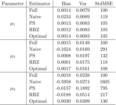
In the second simulation study, we used a nonlinear type regression model with serial correlation. The model is
Y0 =X/3 +Z/3 +e0, Yt= 1 +X/3 +Z/3 +et,fort >1,
independent and identically distributed N(0,1) random variables. The missing indicator rt
follows the following distribution:
P(rt= 1|X, Yt−1, rt−1 = 1) =
1
1 + exp[−2.5−X+{Yt−1−(t−1)}/2]
, (5.55)
and there are no missing data in the baseline year. In this simulation setup, the true mean of
Yt is E(Yt) =t. The parameters of interest again are µt=E(Yt), fort= 1,2,3.
Here we used B = 10,000 Monte Carlo samples of size n= 500 for this simulation. The response rates fort= 1,2,3 are 0.90,0.82,0.74 respectively. The simulation results in Table5.3
show the same tendency as Table 5.2. The relative biases of the variance estimator using the formula in (5.36), fort= 1,2,3, are0.0137,−0.0115,−0.0671respectively. At timet= 3, the relative efficiency of the proposed estimator over the RRZ estimator is 167%, which is greater than 124% of the first simulation study, and it is because the working regression model assumed in the RRZ model does not hold in the sample generated by (5.55).
Table 5.3 Comparison for different methods when n = 500, T = 3 with Monte Carlo sample size 10,000 for simulation study 2.
Parameter Estimator Bias Var StdMSE
µ1 Full 0.0014 0.0079 100 Naive 0.0234 0.0089 119 PS 0.0013 0.0083 105 RRZ 0.0012 0.0083 105 Optimal 0.0014 0.0083 105 µ2 Full 0.0015 0.0149 100 Naive -0.1624 0.0169 291 PS 0.0008 0.0197 132 RRZ 0.0001 0.0175 118 Optimal 0.0017 0.0161 108 µ3 Full 0.0018 0.0238 100 Naive -0.5958 0.0274 1605 PS -0.0157 0.1892 795 RRZ -0.0188 0.0514 217 Optimal 0.0030 0.0309 130
5.7 Conclusion
We have considered the problem of estimating population mean for longitudinal data with monotone missing patterns. The proposed method uses a parametric response model where the response probability at time t depends on the available observations at time t−1, that is, on (X0, Y1, . . . , Yt−1)0. We used a logistic regression model for the response probability, but
the proposed method can be easily extended to other response probability models that use an explicit parametric form for the response probability.
The proposed method makes the best use of all (asymptotically) unbiased estimators avail-able for each wave of the panel survey. The way we combine the information is based on the GMM technique and the resulting estimator is asymptotically optimal among a class of estimators that can be written as linear combinations of the unbiased estimators of the panel estimates for each wave. The proposed method is directly applicable to the case when the baseline year sample is selected with a complex probability sample. Variance estimation using linearization method is relatively straightforward.
The proposed method requires that the missing pattern be monotone. If the proposed method is applied to non-monotone missing patterns, estimation of response probability at time t can be more complicated because Yi,t−1 are not always observed for non-monotone
missing case. Extension of the proposed method to non-monotone missing data will be an important topic for future research.
5.A Proofs and Discussions
5.A.1 Proof of Theorem 5.1
Let hi,t(φt) = ∂logit(pit)/∂φt where logit(p) = log{p/(1−p)}, Hi,t = (ξi,t0 −1, ψi,t0 −1)0.
Throughout the following arguments, unless explicitly pointed out, we shall suppress the no-tation of true parameters φ∗t such that all expectations are evaluated at the true parameters. We shall assume the following regularity conditions.
(C1) The conditional response probabilities are bounded from below uniformly, that is, there exists a fixed positive constantσ such thatpit> σfori= 1, . . . , n;t= 1, . . . , T uniformly.
(C2) The solution ˆφt toSt(φt) = 0 satisfies ˆφt=φ∗t+op(1) fort= 1, . . . , T.
(C3) pit(φt) is twice continuously differentiable in the neighborhood of φ∗t fort= 1, . . . , T.
(C4) X, Yt, ht(φ∗t), ∂ht(φ∗t)/∂φt have finite second moments fort= 1, . . . , T.
(C5) V ar{Hi,T} is nonsingular,E{∂HT/∂φ¯T}exists and is nonsingular.
(C6) There exists a neighborhoodNt ofφ∗t such thatE{supφt∈Ntkht(φt)k}<∞,E{supφt∈Nt
kht(φt)ht(φt)0k}<∞and E{supφt∈Ntk∂ht/∂φtk}<∞fort= 1, . . . , T.
Proof. The optimal Bt∗ that minimizes the variance of ˜E{rtYt/πˆt} −Bt0E˜{ξˆt−1} is given by
V ar[ ˜E{ξˆt−1}]Bt∗ =Cov( ˜E{ξˆt−1},E˜{rtYt/πˆt}).
Let Ui,t(γ) = (µt−ritYit/πit, ξi,t0 −1, ψi,t0 −1)0, where γ = (µt,φ¯0t)0 with ¯φt = (φ01, . . . , φ0t)0.
First of all, conditions Lemma 5.1 (i) (ii) hold by (C1), (C2), (C4). For example, because
πit =Qtj=1pijπ0 ≥σt, |ri,t/πi,t−ri,t−1/πi,t−1| ≤2/σt,E{rtYt2/π2t} ≤E{Yt2}/σ2, E[k(rt/πt−
rt−1/πt−1)Lt−1k2] ≤ 2EkLt−1k2/σ2. Also, (C3) implies (iii), (C5) implies (iv). Note that
pit(1−pit)hi,t = ∂pit/∂φt, thus E{supφt∈Ntk∂pit/∂φtk} ≤ E{supφt∈Ntkhit(φt)k}/4 < ∞,
k∂πit/∂φkk=k∂pik/∂φk
Q
j6=kpij(φj)k ≤ k∂pik/∂φkk. Moreover,k∂{(ri,t−ri,t−1pit)hi,t}/∂φtk
=k −ri,t−1(∂pit/∂φt)h0it+ (ri,t−ri,t−1pi,t)∂hi,t/∂φtk ≤ khi,thi,t0 k/4 + 2k∂hi,t/∂φtk. Therefore,
(C6) implies (v). Note that under logistic response model in (5.24), hi,t =Li,t−1, (C6) would
automatically hold. Although in the following arguments, we adopt the logistic regression model in (5.24), the derivation shall carry through without extra effort. By similar arguments in the remark of Lemma5.1, we have
ˆ ¯ φt−φ¯∗t = −E ∂S¯t( ¯φ∗t) ∂φ¯t −1 ¯ St( ¯φ∗t) +op(n−1/2) ˜ E{ξˆt−1}= ˜E{ξt−1( ¯φ∗t)} −E ∂ξt−1( ¯φ∗t) ∂φ¯t E ∂S¯t( ¯φ∗t) ∂φ¯t −1 ¯ St( ¯φ∗t) +op(n−1/2) ˜ E{rtYtπˆt}= ˜E{rtYt/πt( ¯φ∗t)} −E ∂(rtYt/πt( ¯φ∗t)) ∂φ¯t E ∂S¯t( ¯φ∗t) ∂φ¯t −1 ¯ St( ¯φ∗t) +op(n−1/2).
By similar argument in the remark, (see alsoPierce,1982), we have
E ∂ξt−1 ∂φ¯t =−Cov(ξt−1,S¯t) =−Cov(ξt−1, ψt−1), E ∂S¯t( ¯φt) ∂φ¯t =V ar( ¯St) =nV ar(ψt−1).
Therefore, V ar[ ˜E{ξˆt−1}] =V ar[ ˜E{ξt−1}]−Cov(ξt−1,S¯t)V ar( ¯St)−1Cov( ¯St, ξt−1) +o(n−1) Cov( ˜E{ξˆt−1},E˜{rtYt/πˆt}) =Cov( ˜E{ξt−1},E˜{rtYt/πt}) −Cov(ξt−1,S¯t)V ar( ¯St)−1Cov( ¯St, rtYt/πt) +o(n−1). Let V ar ξt−1 ψt−1 =E ξt−1 ψt−1 ξt−1 ψt−1 0 = VLL,t VLS,t VLS,t VSS,t , VLY,t VSY,t =E ξt−1 ψt−1 rtYt/πt , then Bt∗ = (VLL,t−VLS,tVSS,t−1 VSL,t)−1(VLY,t−VLS,tVSS,t−1VSY,t) +op(1). (5.56) We can writeBt∗ as Bt∗= (I, O) VLL,t VLS,t VLS,t VSS,t −1 VLY,t VSY,t +op(1). (5.57) Notice that E{ri−1ui|Li−1} = 0, E(ri−1u2i|Li−1) = ri−1(1/pi−1), E(ri−1uirj−1uj|Li−1) = 0 fori < j, we have VLL,t =E diag 1 p1 −1 r0 π20L0L 0 0,· · · , 1 pt −1 rt−1 πt2−1Lt−1L 0 t−1 VLS,t =E diag 1 p1 −1 r0p1 π0 L0L00,· · ·, 1 pt −1 rt−1pt πt−1 Lt−1L0t−1 VSS,t =E diag 1 p1 −1 r0p21L0L00,· · · , 1 pt −1 rt−1p2tLt−1L0t−1 VLY,t=E 1 p1 −1 L0 π0 rtYt πt ,· · · , 1 pt −1 Lt−1 πt−1 rtYt πt VSY,t=E 1 p1 −1 p1L0 rtYt πt ,· · · , 1 pt −1 ptLt−1 rtYt πt .
All theV matrices or vectors can be written as the form of diagonal blocks. If V is a matrix, thenV =diag(V(1), . . . , V(t)), wheredim{V(j)}=dim(Lj−1)×dim(Lj−1). If V is a vecotr,
thenV = (V(1)0, . . . , V(t)0)0, wheredim{V(j)}=dim(Lj−1)×1. Then B∗t = (B1∗t
0, . . . , B∗ 1t
where Bj,t∗ ={VLL,t(j)−VLS,t(j)VSS,t−1 (j)VSL,t(j)}−1{VLY,t(j)−VLS,t(j)VSS,t(j)−1VSY,t(j)} = (Idim(Lj−1),0) E rj−1 1 pj −1 1 πj−1Lj−1 pjLj−1 1 πj−1Lj−1 pjLj−1 0 −1 ×E rt πt 1 pj −1 1 πj−1Lj−1 pjLj−1 Yt .
5.A.2 Proof of Theorem 5.2
Proof.
ˆ
Yt,opt= ˜E{rtYt/πˆt} −Eˆ{ξˆt−1}0Bˆt−E˜{ψˆt−1}0Cˆt.
Denote parameterγ = (B, C, φ)0 and γ∗= (Bt∗, Ct∗,φ¯∗t), then define
µ1(γ) =E∗γ{rtYt/πt} −B0Eγ∗{ξt−1} −C0Eγ∗{ψt−1}.
Then under regularity conditions (C1) - (C4), we are able to do the following derivatives,
∂µ1(γ) ∂B γ=γ∗ =Eγ ∗{ξt−1}|γ=γ∗= 0 ∂µ1(γ) ∂C γ=γ∗ =Eγ ∗{ψt−1}|γ=γ∗ = 0.
Moreover, notice that ¯St = nE˜{ψt−1}. Under conditions (C1)-(C6), by the results we have
shown in Theorem 5.1, using the same notations, we have
∂µ1(γ) ∂φ γ=γ∗ =VY S,t−B ∗ t 0 VLS,t−Ct∗ 0 VSS,t To show that ∂µ1(γ) ∂φ
γ=γ∗ = 0, it suffices to show that VSS,t−1VY S,t−VSS,t−1VSL,tBt∗=C ∗ t = (O, I) VLL,t VLS,t VSL,t VSS,t −1 VLY,t VSY,t . (5.58) Note that Bt∗ = (I, O) VLL,t VLS,t VSL,t VSS,t −1 VLY,t VSY,t ,
and we can show the following equality VSS,t−1VY S = (VSS,t−1VSL,t, I) VLL,t VLS,t VSL,t VSS,t −1 VLY,t VSY,t ,
(5.58) then follows. Therefore, the Randles(1982) condition is satisfied, and
ˆ Yt,opt= ˜E(rtYt/πt)− t X j=1 D∗j,t0E˜ rj−1uj 1 πj−1Lj−1 pjLj−1 +op(n−1/2), (5.59) where D∗j,t=E−1 rj−1 1 pj −1 1 πj−1Lj−1 pjLj−1 1 πj−1Lj−1 pjLj−1 0 E 1 pj −1 1 πj−1Lj−1 pjLj−1 rtYt πt .
Let ηt be the random quantity as given in (5.33), then ˆYt,opt = ˜E(ηt) +op(n−1/2). Because ηt
has second moment, by central limit theorem, (5.34) holds. Now we shall show that V ar(ηt)
can be consistently estimated by ˆV = (n−1)−1E˜{(ˆηt−η¯ˆt)2}, where
ˆ ηi,t=ritYit/πˆit− t X j=1 ˆ
Dj,t0 ri,j−1uˆi,j(L0i,j−1/πˆi,j−1,pˆijL0i,j−1)0.
Note that we have already shown ˜E{ηˆt} = ˜E(ηt) +op(n−1/2), it then suffices to show that
˜
E{ηˆtηˆ0t} = ˜E{ηtη0t}+op(1). By (C1), (C2), (C4), (C6), there exists a neighborhood ¯Nt of
¯
φt∗ such that E[supφ¯t∈N¯tkηtk] < ∞, E[supφ¯t∈N¯tkηtη0tk] < ∞. By Lemma 4.3 of Newey and
McFadden (1994), we have ˆDj,t = Dj,t∗ +op(1) and ˜E{ηˆtηˆ0t} = ˜E{ηtηt0}+op(1). Therefore,
ˆ
V = (n−1)−1E˜{(ηt−η¯t)2}+op(n−1) = n−1V ar(ηt) +op(n−1). That is ˆV /{V ar(ηt)/n} =
1 +op(1).
5.A.3 Comment for Remark 5.3
The following comment shows that whether estimatingµX, µ1, . . . , µT simultaneously or not
Let g(X;θ,φ) = ˜ E{r0X/π0} −µX ˜ E{r1Y1/π1} −µ1 ˜ E{r2Y2/π2} −µ2 .. . ˜ E{rTYT/πT} −µT ˜ E{ξT−1} ˜ E{ψT−1} = A(X;θ,φ) B(X;φ) .
We can obtain ˆθ by minimizing ˜Qwith respect to θ, where ˜
Q=g(X;θ,φˆ)0[V ar{g(X;θ,φ)}]−1g(X;θ,φˆ),
which is equivalent to minimizingA(X;θ,φˆ)[V ar{A(X;θ,φˆ)}]−1A(X;θ,φˆ), similar to our dis-cussion in the T = 1 case. Notice that the solution to ˜Q would not change, if we rearrange
B(X;φ) as B(X;φ) = ˜E r0u1 L0 π0 p1L0 r1u2 L1 π1 p2L1 .. . rt−1uT LT−1 πT−1 pTLT−1 . ˜
Qcan be written as ˜Q= ˜Q1+ ˜Q2, where ˜Q2 =B(X; ˆφ)0[V ar{B(X;φ)}]−1B(X; ˆφ) and ˜Q1 is
˜
Q1={A(X;θ,φˆ)−Cov{A(X;θ,φ), B(X;φ)}[V ar{B(X;φ)}]−1B(X; ˆφ)} ×[V ar{A(X;θ,φ)} −Cov{A(X;θ,φ), B(X;φ)}[V ar{B(X;φ)}]−1
×Cov{B(X;φ), A(X;θ,φ)}]−1
× {A(X;θ,φˆ)−Cov{A(X;θ,φ), B(X;φ)}[V ar{B(X;φ)}]−1B(X; ˆφ)}.
Now considerV ar{B(X;φ)}, which would be a matrix of diagonal blocks, that is,
V ar{B(X;φ)}=diag V ar r0u0 L0 π0 p1L0 , . . . , V ar rt−1uT LT−1 πT−1 pTLT−1 .
On the other hand, if we look at Cov{A(X;θ,φ), B(X;φ)}, it is equal to the following lower triangular matrix Cov{E˜(r0X/π0), B(X;φ)} Cov{E˜(r1Y1/π1), B(X;φ)} Cov{E˜(r2Y2/π2), B(X;φ)} .. . Cov{E˜(rTYT/πT), B(X;φ)} = O Cov ˜ E(r1Y1/π1),E˜ ξ0 ψ0 O Cov ˜ E(r2Y2/π1),E˜ ξ1 ψ1 O .. . Cov ˜ E(rTYT/π1),E˜ ξT−1 ψT−1 O .
Therefore, µtcan be estimated by solving
˜ E{rtYt/πˆt} −µt−Covˆ ˜ E(rTYT/π1),E˜ ξt−1 ψt−1 V ar−1 rt−1ut Lt−1 πt−1 ptLt−1 ˜ E ˆ ξt−1 ˆ ψt−1 ,
which is the same as minimizer of Qtin (5.29).
5.A.4 Sketch of Proof for Corollary 5.1
Proof. With similar arguments to the proof of Theorem 5.1, under conditions (C1)-(C8), we
have ˜ EA( ˆξt−1) = ˜EA(ξt−1)−E{E˜A(ξt−1ψt0−1)|FN}[E{E˜A(ψt−1ψt0−1/w)|FN}]−1 ×E˜A(ψt−1/w) +op(n−1/2), ˜ EA(rtYt/πˆt) = ˜EA(rtYt/πt)−E[ ˜EA{(rtYt/πt)ψ0t−1}|FN][E{E˜A(ψt−1ψ0t−1/w)|FN}]−1 ×E˜A(ψt−1/w) +op(n−1/2).
Note thatE{(rit/pit−1)ri,t−1|A,FN}=E[E{(rit/pit−1)ri,t−1|ri,t−1, A,FN}|A,FN] = 0, then
E{E˜A(ξt−1)|A,FN}= 0, E{E˜A(ψt−1/w)|A,FN}= 0, and
Cov{E˜A(ξt−1),E˜A(ψt−1/w)|FN}=E{E˜A(ξt−1ψt−1)0|FN}
V ar{E˜A(ψt−1)/w|FN}=E{E˜A(ψt−1ψ0t−1/w)|FN}
The rest of this proof would follow similarly from the proof of Theorem5.1. One important step is to calculate V ar[ ˜EA{(ξt0−1, ψt0−1/w)0}|FN] and Cov[ ˜EA(rtYt/πt),E˜A{(ξt0−1, ψt0−1/w)0}|FN].
V ar ˜ EA ξt−1 ψt−1/w FN =V ar E ˜ EA ξt−1 ψt−1/w A,FN FN +E V ar ˜ EA ξt−1 ψt−1/w A,FN FN .
We only have to calculate the second term as the first term is 0. For the second term, notice that V ar ˜ EA ξt−1 ψt−1/w A,FN = 1 N2 X i∈A w2iV ar ξi,t−1 ψi,t−1/wi A,FN = N−2P
i∈Aω2iV ar(ξi,t−1|A,FN) N−2Pi∈AωiCov(ξi,t−1, ψi,t−1|A,FN)
N−2P
i∈AωiCov(ψi,t−1, ξi,t−1|A,FN) N
−2P
i∈AV ar(ψi,t−1|A,FN)
.
Again V ar(ξi,t−1|A,FN) can be written as a matrix of diagonal blocks such that it is equal to
diag[V ar{(ri1/pi1−1)ri0Li,0/πi,0|A,FN}, . . . , V ar{(rit/pit−1)ri,t−1Li,t−1/πi,t−1|A,FN}],
where
V ar{(rij/pij −1)ri,j−1Li,j−1/πi,j−1|A,FN}=
Li,j−1L0i,j−1
π2
i,j−1
(1/pij−1)πi,j−1.
Other related terms can be obtained in a similar fashion. Thus
V ar ˜ EA ξt−1 ψt−1/w FN = ˜ VLL,t V˜LS,t ˜ VSL,t V˜SS,t , where ˜ VLL,t=N−2 N X i=1 ωidiag ( Li,0L0i,0 πi,20 (1/pi1−1)πi,0, . . . , Li,t−1L0i,t−1 πi,t2 −1 (1/pit−1)πi,t−1 ) , ˜ VLS,t =N−2 N X i=1 diag p i1Li,0L0i,0 πi,0 (1/pi1−1)πi,0, . . . , pitLi,t−1L0i,t−1 πi,t−1 (1/pit−1)πi,t−1 , ˜ VSS,t=N−2 N X i=1 ω−1i diag
Cov[ ˜EA(rtYt/πt),E˜A{(ξ0t−1, ψt0−1/w)0}|FN] = ( ˜VY L0 ,V˜Y S0 )0, where ˜ VY L=N−2 N X i=1 ωiYi,t (1/pi1−1)L0i,0/πi0, . . . ,(1/pit−1)L0i,t−1/πi,t−1 0 ˜ VY S =N−2 N X i=1 Yi,t (1−pi1)L0i,0, . . . ,(1−pit)L0i,t−1 0 .
Similarly to the diagonal block-wise technique used in the proof of Theorem5.1, we obtain the optimalBt∗= (B∗1t 0 , . . . , Btt∗0)0, where Bj,t∗ ={V˜LL,t(j)−V˜LS,t(j) ˜VSS,t−1 (j) ˜VSL,t(j)}−1{V˜LY,t(j)−V˜LS,t(j) ˜VSS,t(j)−1V˜SY,t(j)} = (Idim(Lj−1),0) ˜ VLL(j) V˜LS(j) ˜ VLS(j) V˜SS(j) −1 ˜ VLY(j) ˜ VSY(j) = (Idim(Lj−1),0) ˜ E wπj−1 1 pj −1 1 πj−1Lj−1 pjLj−1/w 1 πj−1Lj−1 pjLj−1/w 0 −1 ×E˜ w 1 pj −1 1 πj−1Lj−1 pjLj−1/w Yt .
References
Beaumont, J.-F. and Bocci, C. (2009). Variance estimation when donor imputation is used to fill in missing values. Canadian Journal of Statistics, 37:400–416.
Bollinger, C. R. and David, M. H. (1997). Modeling discrete choice with response error: Food stamp participation. Journal of the American Statistical Association, 92:827–835.
Bollinger, C. R. and David, M. H. (2001). Estimation with response error and nonresponse: Food-stamp participation in the sipp.Journal of Business & Economic Statistics, 19:129–141. Cao, W., Tsiatis, A., and Davidian, M. (2009). Improving efficiency and robustness of the doubly robust estimator for a population mean with incomplete data. Biometrika, 96:723– 724.
Fay, R. E. (1992). When are inferences from multiple imputation valid? InProc. Survey Res.
Meth. Sect., pages 227–232. Washington, DC: American Statistical Association.
Flanders, W. D. and Greenland, S. (1991). Analytic methods for two-stage case-control studies and other stratified designs. Statistics in Medicine, 10:739–747.
Hansen, L. P. (1982). Large sample properties of generalized method of moments estimators.
Econometrica, 50:1029–1054.
Hawkes, D. and Plewis, I. (2006). Modelling non-response in the national child development study. Journal of the Royal Statistical Society: Series A (Statistics in Society), 169:479–491. Henmi, M. and Eguchi, S. (2004). A paradox concerning nuisance parameters and projected
estimating functions. Biometrika, 91:929–941.
Horvitz, D. G. and Thompson, D. J. (1952). A generalization of sampling without replacement from a finite universe. Journal of the American Statistical Association, 47:663–685.
Kim, J. K. and Kim, J. J. (2007). Nonresponse weighting adjustment using estimated response probability. Canadian Journal of Statistics, 35:501–514.
Kim, J. K., Navarro, A., and Fuller, W. A. (2006). Replication variance estimation for two-phase stratified sampling.Journal of the American Statistical Association, 101(473):312–320. Kim, J. K. and Rao, J. N. K. (2009). A unified approach to linearization variance estimation
from survey data after imputation for item nonresponse. Biometrika, 96(4):917–932.
Korinek, A., Mistiaen, J. A., and Ravallion, M. (2007). An econometric method of correcting for unit nonresponse bias in surveys. Journal of Econometrics, 136:213–235.
Little, R. J. and Vartivarian, S. (2005). Does Weighting for Nonresponse Increase the Variance of Survey Means? Survey Methodology, 31:161–168.
Little, R. J. A. (1995). Modeling the drop-out mechanism in repeated-measures studies.Journal
of the American Statistical Association, 90:1112–1121.
Manski, C. F. and Lerman, S. R. (1977). The estimation of choice probabilities from choice based samples. Econometrica, 45:1977–1988.
Newey, W. K. and McFadden, D. (1994). Large sample estimation and hypothesis testing. In Engle, R. F. and McFadden, D., editors, Handbook of Econometrics, volume 4, chapter 36, pages 2111–2245. Elsevier, 1 edition.
Pierce, D. A. (1982). The asymptotic effect of substituting estimators for parameters in certain types of statistics. The Annals of Statistics, 10(2):475–478.
Randles, R. H. (1982). On the asymptotic normality of statistics with estimated parameters.
The Annals of Statistics, 10:462–474.
Robins, J. M., Rotnitzky, A., and Zhao, L. P. (1994). Estimation of regression coefficients when some regressors are not always observed. Journal of the American Statistical Association, 89:846–866.
Robins, J. M., Rotnitzky, A., and Zhao, L. P. (1995). Analysis of semiparametric regression models for repeated outcomes in the presence of missing data.Journal of American Statistical
Rosenbaum, P. R. (1987). Model-based direct adjustment. Journal of the American Statistical
Association, 82:387–394.
Rosenbaum, P. R. and Rubin, D. B. (1983). The central role of the propensity score in obser-vational studies for causal effects. Biometrika, 70(1):41–55.
Rotnitzky, A., Robins, J. M., and Scharfstein, D. O. (1998). Semiparametric regression for repeated outcomes with nonignorable nonresponse. Journal of the American Statistical
As-sociation, 93:1321–1339.
Rubin, D. B. (1976). Inference and missing data. Biometrika, 63:581–590.
Shao, J. and Steel, P. (1999). Variance estimation for survey data with composite imputa-tion and nonnegligible sampling fracimputa-tions. Journal of the American Statistical Association, 94(445):254–265.
Tan, Z. (2006). A distributional approach for causal inference using propensity scores. Journal
of the American Statistical Association, 101:1619–1637.
Wun, L.-M., Ezzati-Rice, T. M., Diaz-Tena, N., and Greenblatt, J. (2007). On modelling response propensity for dwelling unit (du) level non-response adjustment in the medical expenditure panel survey (meps). Statistics in Medicine, 26:1875–1884.