FlexPref: A Framework for Extensible Preference
Evaluation in Database Systems
Justin J. Levandoski
1, Mohamed F. Mokbel
2, Mohamed E. Khalefa
3Department of Computer Science and Engineering, University of Minnesota, Minneapolis, MN, USA
1
[email protected], [email protected], [email protected]
Abstract— Personalized database systems give users answers
tailored to their personal preferences. While numerous preference evaluation methods for databases have been proposed (e.g., skyline, top-k, k-dominance, k-frequency), the implementation of these methods at the coreof a database system is a double-edged sword. Core implementation provides efficient query pro-cessing for arbitrary database queries, however this approach is
not practical as each existing (and future) preference method
requires a custom query processor implementation. To solve this problem, this paper introduces FlexPref, a framework for extensible preference evaluation in database systems. FlexPref, implemented in the query processor, aims to support a wide-array of preference evaluation methods in a single extensible code base. Integration with FlexPref is simple, involving the registration of only three functions that capture the essence of the preference method. Once integrated, the preference method “lives” at the core of the database, enabling the efficient execution of preference queries involving common database operations. To demonstrate the extensibility of FlexPref, we provide case studies showing the implementation of three database operations (single table access, join, and sorted list access) and five state-of-the-art preference evaluation methods (k, skyline, k-dominance, top-k dominance, and top-k-frequency). We also experimentally study the strengths and weaknesses of an implementation of FlexPef in PostgreSQL over a range of single-table and multi-table preference queries.
I. INTRODUCTION
Embedding preferences in or on-top of databases has helped realize non-trivial applications, ranging from multi-criteria decision-making tools to personalized databases [1]. Prefer-ence queries give users interesting answers by evaluating their personal wishes according to a certain preference method. In the literature, there exist a large number of preference evalua-tion methods, including top-k [2], skylines [3], hybrid multi-object methods [4],k-dominance [5],k-frequency [6], ranked skylines [7], k-representative dominance [8], distance-based dominance [9],ǫ-skylines [10], and top-kdominance [11]. In general, the point of proposing new preference methods is to challenge the notion of “best” answers. Since the concept of “best” is subjective, there is theoretically no limit to the num-ber of new preference methods that can be proposed. Given the large number of preference methods already proposed, and likely to be created in the future, a fundamental issue behind each method is how it can handle arbitrary queries in a database management system (DBMS) that may contain selection, aggregation, and/or join operations.
This work is supported in part by the National Science Foundation under Grants IIS0811998, IIS0811935, CNS0708604, and by a Microsoft Research Gift
The most common approach for preference evaluation in database systems is theon-topapproach where the preference method is realized as either a stand-alone program or as a database user-defined function. This approach treats the DBMS as a “black box”, where the preference evaluation method is completely decoupled from the database, and hence not concerned with internal database operations (e.g., joins) necessary to retrieve the data (e.g., see [4], [5], [6], [7], [8], [9], [10], [11]). The main advantage of this approach is its simplicity as it only requires the implementation of the preference evaluation method in a separate code base outside the core database engine. However, the efficiency of this approach is limited as it cannot interact with database internal operations, and hence cannot optimize the database query processor to be advantageous to the preference evaluation method [12], [13]. Furthermore, preference evaluation methods may be created assuming that data exists in a specific format (e.g., non-standard index), unaware of how data is physically stored or retrieved from the database.
A much more efficient approach for preference evaluation in database systems is the built-inapproach that tightly couples preference evaluation with the query processor by creating optimized, customized, database operations (e.g., selection, aggregation, and join) for each preference method. The ef-ficiency of this approach over the on-top approach is obvious from the extensive work of injecting ranking and top-k queries inside the database engine for selection queries [14], [2], join queries [15], and sorted list access [16], [17]. However, it is not practical to develop a database system that handleseach exist-ing and future preference method. Given the amount of effort needed to inject top-k operations in database systems [18], it would be hard to replicate this effort for each preference method. From a practical standpoint, supporting each distinct preference method in this manner is impossible for actual database systems, commercial or otherwise.
In this paper, we present FlexPref; an extensible frame-work for preference evaluation in database systems. FlexPref represents a centrist approach to preference implementation that combines the simplicity of theon-top approach with the efficiency of thebuilt-inapproach. The simplicity of FlexPref comes from the fact that integrating a new preference method involves the registration of only three functions that capture the essence of the preference method. The efficiency of FlexPref comes from the fact that once a preference method is inte-grated with the system, it “lives” at the core of the database, coupled with the database engine and its query processor,
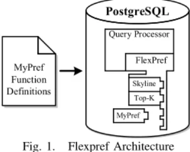
MyPref Function Definitions PostgreSQL Query Processor FlexPref Skyline Top-K MyPref
Fig. 1. Flexpref Architecture
enabling the efficient execution of preference queries involving common database operations.
As depicted in Figure 1, FlexPref is implemented inside the PostgreSQL [19] query processor, and is extensible to arbitrary preference methods. Injecting a preference method into the database requires the implementation of only three functions (outside PostgreSQL) that are then registered with FlexPref. These functions are designed to: (a) specify rules for when a tuple is “preferred” and (b) define rules for how items are added to a current set of preferred objects. Requiring the implementation of only three functions, preference evaluation methods are easier to implement in FlexPref compared to the built-in approach. In fact, FlexPref requires orders of mag-nitude less code. For example, implementing a simple single table skyline evaluation algorithm from scratch in PostgreSQL takes an order of 2,000 lines of code, while with FlexPref embedded in PostgreSQL, skyline implementation is on the order of 300 lines of code.
FlexPref results in efficient realization of preference meth-ods inside the database engine, similar to that of the built-in approach. The main idea is that we tightly couple FlexPref with database operations in a customized manner. For example, we design single table access, join, and sorted list access operations that are customized to FlexPref. Then, any prefer-ence method registered with FlexPref is seamlessly integrated with the FlexPref framework, that is in turn coupled with the query processor. As depicted in Figure 1, it is important to note that only FlexPref touches the query processor while each new preference method is “plugged into” the frame-work. FlexPref raises two fundamental questions regarding the efficient execution of arbitrarypreference queries: (1) Is FlexPref more efficient than the on-top approach?The answer is yes; coupling database operators with general preference criteria implies that a query processor can be optimized to perform early pruning by disregarding data that has no chance of being in a preferred answer set. Such an optimization is not possible with the on-top approach. (2) Is FlexPref more efficient than the built-in approach?. The answer, invariably, is no. Implementing specialized database operations for a specific preference method (e.g., top-k join) will always be more efficient than the generalized extensible case of FlexPref. However, it is impractical to have specialized implementations for eachpreference method. We equate this argument to pre-vious research comparing generalized indexes (e.g., Gist [20]) to that of specialized indexes (e.g., B-tree [21], R-Tree [22]). We demonstrate the functionality of FlexPref through three database operations, namely, single table access, joins, and sorted list access, that are designed to handle any arbitrary preference method integrated in FlexPref. We also provide
case studies for integrating five non-trivial, state-of-the-art preference methods within FlexPref, namely, Skyline [3], Top-k [2], Top-k dominating [11], K-dominance [5], and K-frequency [6]. FlexPref has the potential to provide further functionality beyond the operations discussed in this paper, as it lays the groundwork for further non-trivial, extensible support for preference evaluation in databases, such as special query optimization techniques, uncertain data processing, and indexing. The idea is that any new functionality will need to be realized only oncefor the FlexPref framework, instead of re-implementing it foreachpreference method. We provide ex-perimental evidence examining the strengths and weaknesses of FlexPref, implemented in PostgreSQL, using our three main operations and five case studies, compared toon-topand built-inapproaches.
The rest of this paper is organized as follows. Section II cov-ers related work. Section III describes the usage of FlexPref. The details of the generic functions of FlexPref are described in Section IV. Section V covers preference evaluation in FlexPref through three main database operations. Five case studies of FlexPref are discussed in Section VI. Experimental evaluation of FlexPref is given in Section 7 while Section 8 concludes this paper.
II. RELATEDWORK
Preference methods. Many methods have been proposed for evaluating user preferences over relational data. The two methods receiving the most attention in the literature are skyline [3], [23], [24] and top-k [25], [2], [15], [26]. Other methods have been proposed that evaluate preference queries in a manner different to skyline and top-k, aiming to enhance thequalityof the answer. Examples of these methods include, but are not limited to, hybrid multi-objective methods [4],
k-dominance [5], k-frequency [6], ranked skylines [7], k -representative dominance [8], distance-based dominance [9],
ǫ-skylines [10], and top-kdominance [11]. In this paper, we do not propose a new preference evaluation method. Rather, the goal of FlexPref is to provide asinglegeneralized, extensible preference evaluation framework that allows the integration of any of these preference methods inside a database query processor.
Preference in databases. Much work has gone into em-bedding the notion of preference in database systems from both themodelingandimplementation aspects. Themodeling aspect is concerned more with the theoretical foundation of preference expressions over relational data [27], [28], [29], [30], [1], [31]. In some cases, the model provides rules that define how the model translates into traditional SQL queries. For example, query personalization [1], [32], [33] models preferences using a relational graph, where preferred attributes and relations are given a degree of interest score. Using this graph, SQL queries are injected with the top-k prefer-ences derived from the graph. Meanwhile, PreferenceSQL [30] provides new SQL constructs for expressing preference by defining rules for combining preferences in a cascading or pareto-accumulation manner. Later work defined rules for translating PreferenceSQL into traditional SQL queries [34].
Other work has explored modeling contextual preferences, where the objective is to evaluate preferences that change based on a user’s situation [35], [36], [37].
In terms of preference method implementation, many pro-posed algorithms are not designed to integrate with ad-hoc relational queries involving joins, aggregation, etc [4], [5], [6], [7], [8], [9], [10], [11]. They are implemented “outside-the-box”: completely outside the DBMS or as user-defined functions that sit on-topof a query plan. The closest work to ours investigates integrating preference evaluation algorithms within a database query processor. To this extent, there has been work integrating top-k preferences with selection [3], [2] and join queries [15], and skylines for join queries [15]. Conversely, we do not studycustomimplementations. FlexPref aims to supportanypreference method inside the database en-gine in a general, extensible manner. The FlexPref framework is completely novel in this regard.
III. USINGFLEXPREF
In this section, we show how to: (a) register a new pref-erence method in FlexPref, and (b) how to query a database system, e.g., PostgreSQL, that is equipped with FlexPref. A. Adding A Preference Method to FlexPref
Adding a preference evaluation method to FlexPref requires the implementation ofthreefunctions outside the database en-gine. The details of these functions are covered in Section IV. Once implemented, the preference method is registered using aDefinePreference command, formally:
DefinePreference [Name] WITH [File]
The name argument is the name of the preference method, while the fileargument specifies the file containing the func-tion definifunc-tions.DefinePreferencecompiles the preference code into our framework. This process is depicted in Figure 1 for a preference method “MyPref”.
B. Querying FlexPref
Once a preference method is registered with FlexPref, it can be used in database queries immediately. FlexPref requires the extension of the SQL syntax in order to select the appropriate preference methods and specify their objectives. In this sec-tion, we will first describe the general skeleton of SQL queries in FlexPref, and then describe the specific arguments for our five case studies of preference methods.
1) Query Skeleton: FlexPref adds a Preferring and Usingclause to conventional SQL in order to issue preference queries. A typical query in FlexPref is:
Select [Select Clause]
From [Tables]
Where [Where Clause]
Preferring [Preference Attributes]
Using [method] With [Parameter]
Objectives [Objective]
Here, the method (with objectives) specified in the Using
clause is responsible for selecting the preference evalua-tion method to be applied over the attributes given in the
Preferringclause.
2) Five Case Studies: Using the query skeleton of Flex-Pref, we now give use case examples for five state-of-the-art preference methods, namely, skyline [3], top-k [2], top-k dominating[11],k-dominance[5], andk-frequency[6]. These preference methods are used throughout the rest of this paper to demonstrate the functionality of FlexPref.
Case Study I: Skyline.Theskylinepreference method returns objects in a data set that are not dominated by (i.e., not strictly worse than) any other object in the data. An example query using the skyline method is:
Select *From Restaurant RPreferring
R.price d1 AND R.dist d2 AND R.rating d3
Using Skyline
With Objectives MIN d1, MIN d2, MAX d3;
This query will evaluate the skyline of restaurant data, where the preference objectives require minimizing both price and distance attributes, while maximizing rating.
Case Study II: Top-k dominating. The top-k dominating method ranks each objectQbased on how many other objects it dominates, and returns thekobjects with the highest score. Given the same preference attributes as the previous query, the Using clause for top-k dominating is:
Using Top-K-Domination With K=2
Objectives MIN d1, MIN d2, MAX d3;
Here, the Using clause specifies that: (1) K=2 answers are required and (2) Preference is based on minimizing both price and distance attributes, while maximizing rating.
Case Study III: K-Dominance.Thek-dominancemethod re-definesthe traditional skyline dominance definition to consider onlyk dimensional subspaces, where k is less than or equal to the total number of preference attributes. TheUsingclause for k-dominance is:
Using K-Dominance With K=2
Objectives MIN d1, MIN d2, MAX d3;
For this case, the minimize/maximize objectives are similar to that of top-k domination and skylines. However, K specifies the number of dimensions used to check for dominance be-tween objects. This is in contrast to usual definition ofkthat specifies the number of desired answers.
Case Study IV: K-Frequency.Thek-frequencymethod ranks objects based on their dominance count in all possible dimen-sional subspaces, and returns the k objects with the minimal scores. TheUsingclause for k-dominance is:
Using K-Frequency With K=2
Objectives MIN d1, MIN d2, MAX d3;
The objectives are the same as that of the top-k domination. However, k-frequency evaluates these objectives in a different manner in order to retrieve the “best” objects.
Case Study V: Top-kThetop-kmethod scores each object by combining the object’s attributes using a monotonic ranking function (e.g., summation) that returns a single real value. The
kobjects with the best scores are considered preferred objects. Theusing clause for the top-k method is:
Using Top-K With K=2
Objectives MIN F(d1,d2,d3);
In this clause,K=2answers are required, while the objective is to minimize an object score using monotonic ranking function
IV. FLEXPREFGENERALFUNCTIONS
This section provides the details of the threegeneral func-tions necessary to implement a preference method in FlexPref. To register a certain preference method, e.g., askyline, the user needs to implement these three functions and populate them in the core of FlexPref using theDefinePreferencecommand described in Section III-A. These functions are robust, as they can be used by FlexPref for various efficient query processing techniques as will be described in Section V. We also give five case studies of how these functions can be realized for various preference methods in Section VI.
Before discussing the three functions, we describe two definitions that will be used by our functions and the query processing techniques in Section V
• #define DefaultScore: Each object in FlexPref is associated with a score that is internal to the underlying preference method. It is provided by FlexPref so that the preference method may track the “quality” of each tuple during execution. Defining a default score ensures that each object is assigned a value.
• #define IsTransitive: Indicates whether the method is transitive or not. That is, given objects a,b, and c, if
ais qualitatively “better” thanb, andbis “better” thanc, thenais always “better” thanc. Knowledge of transitivity leads to efficiency, as FlexPref can discard objects during query execution if transitivity holds.
Three general functions need to be implemented by each preference method to be registered with FlexPref.
• PairwiseCompare(Object P, Object Q): Given
two data objects P and Q, update the score of P and return 1 if Q can never be a preferred object, −1 if P
cannever be a preferred object, 0otherwise.
• IsPreferredObject(Object P, PreferenceSet
S): Given a data objectP and a set of preferred objects
S, return true if P is a preferred object and can be added toS,false otherwise.
• AddPreferredToSet(Object P, PreferenceSet
S): Given a data objectP and a preference set S, add
P to S and remove or rearrange objects from S, if necessary.
These functions break down preference evaluation into a set of modular operations that need not be aware of query processor specifics. FlexPref abstracts preference evaluation into two main operations: (1) pairwise comparison of two objects (PairwiseCompare) and (2) comparison of an object with one ore more objects in the current preference set (IsPreferredObject). Though these two functions could be enough for preference registration, FlexPref also provides a third manipulation function, AddPreferredToSet, to allow maximum flexibility and efficiency for the implemented prefer-ence method. For example, each preferprefer-ence method may keep the setSsorted in a manner advantageous to the execution of IsPreferredObject. For preference methods that requirek
answers, AddPreferredToSet has the ability to add a new object while removing an old object to ensure that only k
objects exist in S.
In terms of the scope, FlexPref is able to support a range of qualitative (i.e., skyline) and quantitative (e.g., top-k/ranking) preference methods, as will be discussed in Section VI. If any preference method can reliably define answers by comparing tuples pairwise and/or comparing a tuple to a current preferred set, then it is supported by FlexPref. In general, we envision any preference model/method whose semantics define impera-tive steps that determine whether a tuple is preferred will work in FlexPref.
V. PREFERENCEEVALUATION INFLEXPREF
This section explores the details of preference evaluation in FlexPref that uses the three main functions, PairwiseCompare, IsPreferredObject, andAddpreferredToSet, described in Section IV. We will first present single table access, i.e., selection queries over single table, in FlexPref in Section V-A. Then, in Section V-B we discuss how FlexPref is optimized to process multi-table queries, i.e., join queries. Finally, we discuss a query case when the input is represented as a set of sorted lists (i.e., indexes) in Section V-C. Without loss of generality, the examples throughout the rest of this paper use numeric data. However, FlexPref is compatible with methods for preference evaluation over other data types (e.g., partially-ordered domains [38]).
A. Single-Table Access
Single table access selects a set of preferred objects from a single table. All the query examples given in Section III refer to a single table access where the objective is to retrieve the set of preferred restaurants, according to a certain preference criteria, where all the information is stored in a single tableR. We propose a block-nested loop (BNL) algorithm to execute single-table preference evaluation. We assume data is not indexed, thus a BNL algorithm is necessary (index access is discussed in Section V-C). The main idea is to compare tuples pairwise while incrementally building a preferred answer set. During execution, a data object P may be found to be domi-nated (i.e., guaranteednever to be a preferred answer). If the underlying preference method istransitive,P is immediately discarded and not processed further, thus leading to more efficient execution.
Algorithm 1 outlines the main steps of single-table prefer-ence evaluation in FlexPref. Underlined functions and defini-tions refer to those funcdefini-tions and definidefini-tions that should be implemented separately for each preference method registered with FlexPref, as described in Section IV. While simple, this single execution framework is very powerful as it can ac-commodate myriad preference evaluation methods. As proof, Section VI will cover the implementation of five state-of-the-art preference methods in this framework with execution examples. It is important to note here that Algorithm 1 is generic in the sense that it executes without knowledge of the general preference function details.
The input to Algorithm 1 is a reference to a single database table T while the output is the final set of preferred objects
Algorithm 1 Single Table Access in FlexPref
1: FunctionSingleTableAccess(TableReferenceT) 2: Preference SetS←Φ
3: for eachObjectPinTdo
4: Pscore←DefaultScore 5: for eachObjectQinTdo
6: cmp←PairwiseCompare(P,Q) 7: ifcmp = 1then
8: ifQ∈SthenremoveQfromS
9: ifIsTransitivethendiscardQfromT
10: end if
11: ifcmp = -1then
12: ifIsTransitivethendiscardPfromT
13: Read next objectP(go to line 3)
14: end if
15: end for
16: ifIsPreferredObject(P,S)thenAddPreferredToSet(P,S) 17: end for
18: return S
S to empty. Next, we loop over table T in a block-nested fashion. Object P is read in the outer loop, where definition DefaultScoreassigns its initial score, while objectQis read in the inner loop. Each pair of objects P and Q are com-pared pairwise using the generic functionPairwiseCompare, where the score of object P is updated accordingly. If PairwiseComparereturns 1 (i.e.,Qcan never be a preferred object), and Q currently exists in the preferred set S, then
Q is removed from S. Further, if the preference method is transitive, Q is discarded from tableT mainly for efficiency sake. Due to transitivity, an object that is dominated by Qis also dominated byP, thus there is no need to trackQ. In the case that the underlying preference method is not transitive, we must still consider Q as it may invalidate other objects with which it has not yet been compared. On the other hand, if PairwiseComparereturns -1, thenPcan never be a preferred object. If transitivity holds,Pis discarded from tableT and the next object in the outer loop is read immediately. The argument here is similar to the case of removingQshould the underlying preference function be transitive. Finally, If object P is not discarded in the inner-loop, we call IsPreferredObjectto verify ifP is part of the preference answer. As we will see in Section VI, this is usually a very simple function that performs an O(1) check based on the properties of P and S without the need to iterate over S. If this function returnstrue, P is added to S. The algorithm concludes by returningSafter the block-nested loop execution finishes.
Performance factors. The complexity of the single-table access function is mainly influenced by the preference method’s transitive property. If the method exhibits transitivity, the complexity of Algorithm 1 is O(n) in the best case and
O(n2)
in the worse case. If the method isnottransitive, clearly Algorithm 1 isO(n2)
. Of course, complexity is also influenced by the efficiency of the generic function implementation(s). B. Multi-Table Access
The join operation is one of the most common, and ex-pensive, operations of a DBMS query. Thus, joins will likely be common in preference queries when run on a DBMS. For example, consider a preference query asking about restaurant attributes price, distance, and rating, where price and distance are stored in the same table while the rating information is
R S
Preference Evaluation
(a)Naive join
R S Preference Evaluation Pruning Pruning (b)Join in FlexPref Fig. 2. Join operator
stored in a separate table that may be maintained by a third-party. In this case a join is necessary to fulfill the preference query. We now discuss how FlexPref handles join queries in an efficient manner. We donotassume that input data is sorted or stored in a particular index, thus our method is applicable to any join method (e.g., hash join, index-nested loop) over arbitrary join predicates. For presentation purposes, we discuss the case of a single binary join. However, the concept can be extended to m-way joins or a tree of binary joins.
Figure 2(a) depicts a naive join-then-evaluate strategy to execute join preference queries for two tablesR and S. The idea is to perform a complete join over the two input tables followed by a preference evaluation over the join result. This approach is inefficient, as it does not attempt to optimize the underlying join operator. FlexPref improves upon this naive execution strategy by using the preference criteria functions toprunetuples from the join input that are guaranteed not to be in the final answer. Figure 2(b) gives the FlexPref strategy for handling join queries where pruning is performed at all join inputs, then, a final preference evaluation is performed after joining the non-pruned tuples from each table. Pruning enhances join performance for two main reasons: (a) the amount of data to be joined from input tables is greatly reduced due to pruning the input data, and (b) the amount of data processed by the final preference evaluation after the join is reduced based on the multiplying factor of the join.
Algorithm 2 outlines the main steps for join operations in FlexPref where the input is two tables,RandS, to be joined while the output is the set of preferred objects. First, R and
S are pruned by applying the single table access algorithm (Algorithm 1) to each join-key group in both tables. For example, consider the tablesRandSin Figure 3(b). Assuming ID as a join key, table S contains four groups a,b, c, and d
that contains three, three, one, and one tuple(s), respectively. Also, tableRtrivially contains four single-tuple groups. In this case, single table access would be performedlocallyover each group inS only, asR’s groups contain only a single tuple. By doing so, and according to the underlying preference method, several tuples from each group inScould be pruned, and thus, do not need to be joined with tuples inR. This main idea is that we guarantee that these tuples cannot be preferred objects. Pruning in Algorithm 2 works for the following reason. For each local join-key group, assume we have a set of preferred tuplesP and non-preferred tuples N. We can say that tuples inP are qualitatively better than tuples inN in each join-key group. Given two tablesRandS, the tuples in each join-key group ofS will join with the sametuples in R. If the pruned tuples N inS are qualitatively worse than those inP, then
Algorithm 2 Multi-Table Access in FlexPref
1: FunctionMultiTableAccess(TableR, TableS)
2: Rpruned←PruneR: apply functionSingleTableAccessto each join-key group
inR.
3: Spruned←PruneS: applySingleTableAccessto each join-key group inS. 4: J←Join overRprunedandSprunedusing any join method.
5: return SingleTableAccess(J)/* Algorithm 1 */
tuples in N cannot become qualitatively better once joined with the same data as the tuples inP. Thus, the pruned tuples
N can never be part of the preference query answer.
Once the pruning is done locally for each group in tables
R andS, the rest of the entries in both tables, Rpruned and
Spruned, are joined together using any join method (Line 4 in
Algorithm 2). Finally, FlexPref performs another single table access over the entire join resultJ. This is mainly because the non-pruned tuples formR andS have not yet been compared against each other. The result of this step is the final result of the preference query.
Performance factors. Performance of the multi-table pref-erence join is affected by four main factors. (1) Group By, if objects are not already sorted by their join key, a group by operation is necessary. (2) The complexity of single-table algorithm as it operates on each group. Note that this operation can be donein parallel, as each join-key group is independent of one another. (3) The join algorithm. FlexPref can use any available join method, thus complexity is influenced by the most efficient join algorithm available. (4) The final single-table algorithm operating on the join result. In general, pruning before the join reduces the overall complexity of the join-then-evaluate operation. However, pruning is not always optimal. For instance pruning is not effective in a 1:1 join, as no tuple can be pruned. Section VII experimentally evaluates pruning effectiveness; we omit an in-depth analysis for space reasons. C. Sorted List Access
Availability of sorted attribute lists, or ordered indexes (e.g., B+-tree), allow for efficient preference evaluation. The idea is that complete preference answer generation can be guaranteed after reading only aportion of the sorted data, thus reducing the I/O overhead compared to query processing over unsorted or non-indexed data. Figure 3(c) gives an example of this model where three-dimensional data is presented as three separate 2-ary lists where each list: (a) includes the tuple ID, and (b) is sorted based on its attribute. Note that sorted lists are also an abstraction of an ordered index, such as a B+-tree. Several techniques have been proposed in the literature to take advantages of the sorted lists in preference evaluation, e.g., top-k [15] and skyline [39]. As efficiency is one of the main goals of FlexPref, this section presents a generic algorithm for preference evaluation dealing with sorted lists. Sorted list evaluation requires one extra function be registered with FlexPref.
The main idea behind sorted list access in FlexPref is as follows: (1) Tuples are read, one-by-one, from each list in a round-robin fashion. During this time, we incrementally create a listP ofpartialobjects. This list stores theidof each tuple read so far, along with all values of the tuple that have been
Algorithm 3 Sorted List Access in FlexPref
1: FunctionGeneralSortedAccess(Lists[n],M) 2: stop←false;count←0
3: Partial SetP←Θ 4: ∀i≤nO[i]=Θ; F[i]=Θ 5: whilestop=falsedo
6: Read next tupletfrom Lists[i] in round-robin order
7: iffirst value read from List[i]thenF[i]=t.val
8: O[i]=t.val
9: Update/Add tuples toPby combiningtwith existing tuples ont.id
10: ifcount=Mthen
11: stop←StopSortedEval(P,O,F);count←0 12: else
13: incrementcount
14: end if
15: end while
16: for eachincomplete pointq∈Pdo
17: ∀js.t.jis an incomplete dimension ofq, make random access to Lists[j] to
completeq
18: end for
19: return SingleTableAccess(P)/* Algorithm 1 */
read. For example, consider reading one point from each table
D1-D3in Figure 3(c). In this case,P would store two objects: (a,5, ,3) and (b, ,2, ). (2) Round-robin processing ends once a stopping condition is met. This condition is defined by an extensible function, provided by the preference function implementation. (3) After stopping, all partial tuples inP are “completed” by making a random access to each sorted list to fill in missing attributes. To complete an object (a,5, ,3), table D2 would be probed to form (a,5,3,3). (4) Finally, we perform a final preference evaluation over the listP.
To realize this idea, and to take advantage of sorted lists, FlexPref requires that each preference method defines the following function in addition to the three functions described in Section IV.
• StopSortedEval(Set P, Object O, Object F):
Given a set of partial objects P and two virtual objects
O and F, return whether objects currently in P, once completed, are sufficient to perform preference evaluation.
The argumentsO andF inStopSortedEval, store the last and first values read form each input list, respectively. For example, reading round-robin twice from each listD1toD3
in Figure 3(c) will produceO=(7,3,3) andF=(5,2,3). Algorithm 3 outlines the main steps of sorted list preference evaluation in FlexPref that takes as input a reference to n
decomposed relations (Lists), sorted by attribute value (i.e., sorted lists). Each tuple in a list has two attributes, t.id
and t.value; we assume tuples are combined using t.id. The algorithm also takes as input an integer M, used for efficiency purposes to restrict the number of calls to function StopSortedEvalto everyMthlist access. Initialization sets
a boolean value stop to false, an integer count to zero, and partial setP along with virtual objectOandF tonull(Lines 2 to 4). Round-robin processing then starts, and continues until the booleanstopis set to true by StopSortedEval. A tuple
t is read from the current round-robin input list i, and if it is the first tuple read from i, the ith dimension of F is set tot.value. Meanwhile the ith
dimension ofO is also set to
t.value(Lines 7 to 8). One or multiple tuples are then updated or added to P based on combining t with previously-read tuples based ont.id. IfcountequalsM, the booleanstopis set
by calling extensible function StopSortedEval and count
is reset to 0. Otherwise, count is incremented and round-robin processing continues (Lines 9 to 14). After round-round-robin processing, all objects in P are then “completed” by making a random access to the necessary lists(s) (Lines 16 to 18). Sorted access processing concludes by performing single-table preference evaluation over set P using the algorithm outlined in Algorithm 1 (Line 19).
The method used to build partial objects (Line 9 in Algo-rithm 3) can be implemented in many ways. For robustness, FlexPref builds partial objects by abstracting the operation as an m-way symmetric hash join join [40] between m decom-posed (i.e., 2-ary) relations. The idea behind the symmetric hash join is to store a hash table for each input list i. When a tuple t is read from list i, it is hashed to table i using the value of its join attribute. Tuple t is then used to probe all other hash tables to produce partial (or full) objects.
Performance factors. Performance of sorted list access is influenced by two main factors. (1) The number of sorted accesses. In the worse case, a total of m∗n sorted reads are required (average case is mn2 ), wherem is the number of
attributes and nthe number of objects. (2) The efficiency of the generic StopSortedEvalfunction implementation.
VI. CASESTUDIES
In this section, we provide five case studies for inject-ing five state-of-the-art preference evaluation methods in FlexPref, namely, skyline [3], top-k dominating [11], k-dominance [5], k-frequency [6], and top-k [2]. We chose these five case studies carefully to cover a wide spectrum of preference methods. In particular,skylinerepresents transi-tive dominance-based preference methods,k-dominance repre-sents non-transitive dominance-based preference methods, top-krepresents ranking-based preference methods,top-k dominat-ingrepresents preference methods that combine ranking-based and dominance-based preferences, andk-frequencyrepresents methods that propose object rankings that do not require a specific function, but base their scoring on inherent properties of an object (e.g., attribute correlation and subspace search). Per our discussion in Section IV, FlexPref supports any pref-erence method that can define answers by comparing tuples pairwise and/or comparing a tuple to a current preferred set.
For each preference method, we first describe its func-tionality. Then, we cover the implementation of the three general functions described in Section IV. The summary of all functions for the five case studies is given in Table I. Finally, we give illustrative examples, using Figure 3, for single table, multi-table, and sorted list access. Due to space, we provide and in-depth example for the skyline case study, and more summarized examples for subsequent case studies.
A. Case Study 1: Skylines
Given a dataset D, the objective of skyline preference evaluation [3] is to find the set of objects S that are not dominated by any other object in D. An object P is said to dominate an object Q if P is better than or equal to Q
in all dimensions, and strictly better than Q in at least one
dimension. For example, in Figure 3(a) object a dominates objecteas it is better (i.e., less) in all the three dimensions.
1) General Function Implementation: A skyline implemen-tation in FlexPref is given in the second column of Table I. Skyline evaluation does not rank objects. Thus, within our framework, the skyline score of an objectP is binary and is set to one ifP is not dominated, and zero otherwise. Initially, each object is assumed to be a skyline, thus, each object has a default score of one. Furthermore, skylines exhibit the transitive property, thus its transitive definition is set totrue.
Function PairwiseCompare changes the score of P to zero only if it is dominated, and returns the appropriate value based on the dominance relation between P and Q, i.e., if P is dominated it cannot be a preferred object, and vice versa. Q’s score is not updated in PairwiseCompare per the function definition given in Section IV. Function IsPreferredObject does not need the reference set S to determine if P is a preferred object. Instead, it only returns true if Pscore is one, i.e., P was not dominated by any
object. FunctionAddPreferredToSet simply appends P to the end of setS. The stopping condition forStopSortedEval can be based on previous research in distributed skyline query processing [39]. This condition is: stop once there is a complete object Q in set P. At this stopping point, the complete objectQis equal to, or dominates, the virtual object
O. Furthermore, any new object added toP cannot be better thanO, thus only objects currently inPare skyline candidates. 2) Preference Evaluation: Single Table Execution. Con-sider the three-dimensional data in Figure 3(a). First, objecta
is read, given a default score of 1, and compared pairwise with all other objects using PairwiseCompare. Function PairwiseComparereturns -1 whenais compared with object
b, 0 when compared to c, and -1 when compared to dande. Thus,b,c, andd are discarded from the data set. Since a is not dominated, functionPairwiseComparedoes notchange
a’s score to 0. Thus,IsPreferredObjectreports thatacan be added to the preference answer. Object cis then read and also found to be a preferred answer (as it is not dominated bya, the only object left in the data set). After processingc, no objects are left in the data set and execution terminates. Objectsaandc exist in the preference set, each with a score of one, as given in the skyline answer in Figure 3(a).
Multi-Table Execution. In Figure 3(b), pruning removes tuples (a,5,5) and (b,8,8) from table S prior to the join. These tuples are not skylines within their join-key groups. Furthermore, these tuples cannot possibly be skylines when joined with their corresponding tuples (a,5,5) and (b,7,2) in tableR. For example, joined tuple (a,5,3,5,5) will at least be dominated by members of its same join group: both (a,5,5,3,4) and (a,5,5,4,3). Similarly, joined tuple (b,7,2,8,8) would be dominated by both (b,7,2,4,2) and (b,5,5,4,3).
Sorted Table Access. Round-robin processing can stop after five reads for the data in Figure 3(c). At this point, set P
contains objects (a,5,3,3) and (b,7,2, ), while objectOequals (7,3,3) and object F equals (5,2,3). Clearly, any new object added toP cannot be better than virtual objectOdue to sorted access, and any new object added toP will be dominated by the complete objecta.
ID d1 d2 d3 a 5 4 3 b 6 5 3 c 7 2 4 d 8 6 3 e 10 5 11 Skyline (a,1),(c,1) Top-K Dominating (a,3), (b,2) K-Dominance (a,1) K-Frequency (a,1), (c,3) Top-K (a,3.3), (b,3.5) (a) Single-table example
ID R d1 d2 a 5 3 b 7 2 c 8 5 d 10 4 ID S d3 d4 a 3 4 a 4 3 a 5 5 b 4 2 b 3 6 b 8 8 c 3 8 d 11 10 (b) Arbitrary join data
ID d1 a 5 b 7 c 8 d 10 ID d2 b 2 a 3 d 4 c 5 ID d3 a 3 c 3 b 4 d 11 e 12 f 13 f 7 e 8 f 12 e 13 (c) Sorted lists Fig. 3. Case study example data
B. Case Study 2: Top-K Dominating
Given a data set D, the objective of top-k dominating preference evaluation [11] is to score each object P by its dominance power, i.e., the number of objects it dominates. Here, the dominance definition is the same as the skyline method. The preference answer contains the k objects with the highest score (i.e., the objects that dominate the most other objects). As an example, consider objects a and c in Figure 3(a). Object a has a score of three, as it dominates objects b, d, and e. Object c has a score of one as it only dominates e. Object preference is based solely ondominance power, thus non-skyline objects can be preference answers.
1) General Function Implementation: A top-k dominat-ing implementation in FlexPref is given in the third col-umn of Table I. Each object is given a default score of 0, and IsTransitive returns true. When function PairwiseCompare finds that P dominates an object Q, it increments P’s score by one. An object can never be ruled out of the preference answer using pairwise comparison, since
P’s score must be calculated through comparison with all ob-jects, thus PairwiseCompare always returns zero. Function IsPreferredObjectreturns true ifP has a score superior to any of the currentk objects inS, or ifS contains less thank
objects. FinallyAddPreferredToSetaddsP in sorted order in S, removing the old kth object if applicable. A stopping
condition for StopSortedEval can be: stop once there are
k complete objects in set P. While it is possible that some incomplete objects in P will be superior to the complete
k objects, this stopping condition at least ensures that the complete k objects dominate any objects not yet added to
P. The unseen objects are equal-to or dominated by object
O, which in turn is equal-to or dominated by each of the k
complete objects.
2) Preference Evaluation: The top-kdomination answer is given in Figure 3(a) assuming k = 2. In Figure 3(b), top-k
domination pruning removes fromS tuples (a,5,5) and (b,8,8) both with scores of zero. These pruned tuples are not in the top-2 in theirlocaljoin-key groups. Meanwhile, sorted round-robin processing can stop after nine reads for the data in Figure 3(c). At this point, set P contains objects (a,5,3,3), (b,7,2,4), (c,8, ,3), and (d, ,4, ), while objectsOequals (8,4,4) and object F equals (5,2,3).
C. Case Study 3: K-Dominance
Given a data set D and a valuek,k-dominance preference evaluation [5] finds the set of objects S that are not
k-dominated by any other object inD.k-dominant queries are similar in spirit to skyline queries, except for the relaxed notion of dominance: ann-dimensional objectPis allowed to dominate another object Qon anyk≤ndimensions. When
k=n, a k-dominant query reverts to a skyline query. As an example, consider objectsa andc in Figure 3(a). Fork= 2, objecta k-dominates objectc sinceais better in dimensions
d1andd3(less is better). However, whenk= 3neither object dominates the other as in the case of skylines.
1) General Function Implementation: A k-dominance im-plementation in FlexPref is given in the fourth column of Table I. As k-dominance does not rank objects, each object can either have a score of one if it is not k-dominated, zero otherwise. Also, k-dominance is not transitive as circular dominanceis possible: an objectxcank-dominate an object
y, y can k-dominate an object z, and z can k-dominate x. Thus, theIsTransitiveproperty is set tofalse. The function PairwiseComparechanges the score ofP to zeroonlyif it is
k-dominated byQ, and returns the appropriate value based on dominance relation betweenP andQ.IsPreferredObject does not need to reference set S to determine if P is a preferred object, and returns true if P’s score is 1 (i.e., P
is not k-dominated). Function AddPreferredToSet simply appends P to the end of set S. A stopping condition for StopSortedEval is: stop once set P contains an object Q
with at mostk−1incomplete dimensions, andQk-dominates virtual object O, and O does not k-dominate Q (where the value ∞ is substituted for the incomplete dimensions of Q). Having an objectQwith at mostk−1incomplete dimensions ensures that it cannot bek-dominated on these incomplete di-mensions by an object not yet added toP. Furthermore, since
Q k-dominates virtual object O, but O does not k-dominate
Q, then any object not yet added toP is guaranteed to bek -dominated byQ. Thus thek-dominant answer candidates must exist inP. We note that for multi-table execution, where tables
R and S have contain dR anddS dimensions each, pruning
computes the dR and dS-dominant answer, and then the k
-dominant answer in the final (i.e., root) preference evaluation. 2) Preference Evaluation: The k-dominance answer is given in Figure 3(a) assumingk= 2. In Figure 3(b), pruning will remove from tableStuples (a,5,5) and (b,8,8), as they are
k-dominated within their join-key groups. Similarly, round-robin processing can stop after five reads for the data in Figure 3(c), where setPcontains objects (a,5,3,3) and (b,7,2, ) while objectO equals (7,3,3) and objectF equals (5,2,3).
Skyline [3] Top-kDominating [11] K-Dominance [5] K-Frequency [6] Top-K[3]
IsTransitive Returntrue Returntrue Returnfalse Returntrue Returntrue
DefaultScore Return 1 Return 0 Return 1 Return 0 Return 0
PairwiseCompare IfP dominatesQ, return 1. IfQ dom-inates P, update
Pscoreto 0 and
re-turn -1. Otherwise, return 0
IfPdominatesQ, incre-mentPscore by 1.
Re-turn 0
IfPk-dominatesQ, re-turn 1. IfQk-dominates
P, setPscoreto 0 and
return -1. Otherwise, re-turn 0.
Increment Pscore based on
the distinct sub-dimensions whereQ dominates P. Re-turn 0.
Return -1
IsPreferredObject If object score
Pscore equals
1, return true. Otherwise return false.
If the cardinality ofSis less than k or Pscore
is superior to the kth object’s score in S, re-turntrue. Otherwise, re-turnfalse.
If object scorePscore
equals 1, return true. Otherwise return false.
If the cardinality ofSis less thankorPscoreis superior
to the kthobject’s score inS, returntrue. Otherwise, return false.
Assign a score to Pscore using
ranking functionf. If the cardinal-ity ofSis less thankorPscore
is superior to the kthobject’s score inS, returntrue. Otherwise, return false.
AddPreferredToSet Add objectPto the end of setS.
IfShas a cardinality of
k, remove the kthobject
fromS. AddPtoSin sorted order byPscore.
Add objectPto the end of setS.
IfS has a cardinality ofk, remove the kth object from
S. AddPtoSin sorted order byPscore.
IfShas a cardinality ofk, remove the kthobject fromS. AddPto
Sin sorted order byPscore. StopSortedEval Stop once there is a
complete object Q
in setP
Stop once there are k
complete objects in set
P.
Stop once set P con-tains an objectQ with at mostk−1 incom-plete dimensions, andQ
k-dominates virtual ob-jectO, andOcannot k-dominateQ.
Stop once there is a complete objectQin setP.
Stop once there are k complete objects in P that have scores less than or equal-to a given thresh-old value T.T= MIN(f(O[1],F[2]
· · ·,F[n]), f(F[1],O[2],· · ·,F[n]),
f(F[1],F[2]· · ·,O[n])).
TABLE I
REALIZING FIVE PREFERENCE METHODS INFLEXPREF
D. Case Study 4: K-Frequency
Given a data set D, k-frequency preference evaluation [6] scores each objectP by itsdominated subspaces: the number of possible sub-dimensions in which P is dominated. The preference answer contains the k objects with the lowest score (i.e., the objects that are dominated in the least number of possible sub-dimensions). As an example, object a in Figure 3(a) has a score of one, since it can only be dominated in a single sub-dimension (d2by objectc). Meanwhile, object
e has a score of 7, since it is dominated in all possible sub-dimensions by object a (i.e., {d1}, {d2}, {d3}, {d1, d2},
{d1, d3},{d2, d3},{d1, d2, d3}).
1) General Function Implementation: A k-frequency im-plementation in FlexPref is given in the fifth column of Table I. Each object is given a default score of zero, and IsTransitivereturns true. Dominant sub-dimension count-ing must be performed carefully fork-frequency. For instance, in Figure 3(a) objectcis dominated on overlapping dimensions by different objects. That is,cis dominated in sub-dimensions ({d1},{d3},{d1, d3}) by object a, and sub-dimension {d3}
by objectd. Clearly, over-counting dominated sub-dimensions is an issue. Thus, function PairwiseCompare must have access to an extra data structure that stores the dominated sub-dimensions for each objectP. Tracking these sub-dimensions ensures that an object is scored correctly, i.e., distinct sub-dimensions can be extracted and counted. So, Function PairwiseCompareupdatesPscore based on thedistinct
sub-dimensions where Q dominates P. An object can never be ruled out of the preference answer using pairwise comparison since P’s score must be calculated through comparison with all objects, thus PairwiseCompare always returns zero. Function IsPreferredObjectreturns true ifP has a score superior to any of the current kobjects in S or ifS contains less than k objects. AddPreferredToSet adds P in sorted order in S, removing the old kth
object if applicable. A stopping condition forStopSortedEvalis:stop once there is a complete objectQin setP. This is the same stopping case as
skylines. However, this condition guarantees that an interesting set of objects exists inP, as any objectnot yet added toP is guaranteed to be equal-to or dominated by the complete object
Q(much like the skyline case). Thus, any object not in P is guaranteed to be dominated in all possible sub-dimensions, meaning that all unseen objects will have the same score. If there are not yet kobjects in P when the stopping condition is met, then any arbitrary objects can be added to P as they have the same score.
2) Preference Evaluation: Thek-frequency answer is given in Figure 3(a) assuming k = 2. In Figure 3(b), k-frequency pruning will remove from tableStuples (a,5,5) and (b,8,8), as they both have local scores of three, i.e., they are dominated in all possible subspaces. Round-robin processing can stop after five reads for the data in Figure 3(c). At this point,P contains objects (a,5,3,3) and (b,7,2, ), while object O equals (7,3,3) and object F equals (5,2,3).
E. Case Study 5: Top-K
Given a set of dataD, top-kpreference evaluation [2] scores each data objectP using a monotonic ranking functionf. The preference answer contains the k objects with the minimum score. A monotone functionf takes as input multiple attribute values of and objectP and returns a single real number as its score. For example, for objectain Figure 3(a) and a monotone functionf=(101 ∗(d1 +d2) +
4
5∗d3),a’s score is 3.3.
1) General Function Implementation: A top-k implemen-tation in FlexPref is given in the last column of Table I. Each object has a default score of zero, and IsTransitive returnstrue. Top-kdoesnotrely on pairwise comparison since an object’s score is determined using only its own attributes. Thus,PairwiseComparereturn -1 by default; doing so will cause the inner loop to be broken in Algorithm 1, as this scan is not needed. IsPreferredObject computes object
P’s score using a monotonic ranking functionf, and returns true if P has a score superior to any of the current k
AddPreferredToSetadds P in sorted order inS, removing the old kth object if applicable. A possible stopping
con-dition for StopSortedEval is based on previous research that defines threshold score for efficient top-k joins over sorted lists [15]. Specifically, the condition is:stop once there are k complete objects in P that have scores less than or equal-to a given threshold value T. Threshold T is a lower-bound on the scores of any object not seen so far in set P, defined as MIN(f(O[1],F[2],· · ·,F[n]), f(F[1],O[2],· · ·,F[n]),
f(F[1],F[2],· · ·,O[n])). That is, the minimum of the scores taken from combining the last value seen from each input with the first values read from every other input.
2) Preference Evaluation: The top-k answer is given in Figure 3(a) for k = 2, where we aim to minimize scores based on a ranking function that sums all attribute val-ues. In Figure 3(b), pruning will removes from S tuples (a,5,5) and (b,8,8) with scores 10 and 16, respectively. These pruned tuples are not in the top-2 in their join-key groups. Round-robin processing can stop after 12 reads for the data in Figure 3(c). At this point, set P contains (a,5,3,3), (b,7,2,4), (c,8,5,3), (d,10,4,11), whileO=(10,5,11),F=(5,2,3), and threshold T = 13.
VII. EXPERIMENTALEVALUATION
In this section, we experimentally evaluate the perfor-mance of FlexPref. Our experiments involve the following implementations: (1) The skyline, k-dominance, and
top-k preference evaluation methods implemented in FlexPref according to the function definitions given in Section VI. These implementations are denoted FlexSKY, FlexKDOM, and
FlexT K, respectively. (2) The custom implementations of the
skyline block nested loop operator (CustSKY) [3] and the
two-scan K-dominance algorithm (CustKDOM) [5]. We also
implemented the custom multi-relational skyline join operator (JCustSKY) [41] in order to fairly evaluate our multi-relational
preference execution framework. These custom implementa-tions make for the fairest comparison against our framework as they do not assume sorted or indexed data. We note that for the case of top-k, no custom implementation exists that assumes completely unsorted/unranked input [18]. An exception to this claim is the case involving sorted list access, which we discuss in Section VII-B. We perform experiments for three query scenarios: (1) Multi-table access (Section VII-A), (2) Sorted list access (Section VII-B), and (3) Single table access (Section VII-C),
Our FlexPref framework, along with the custom skyline join algorithm [41], are implemented in the backend execu-tor (query processor) of the PostgreSQL 8.3.5 open-source database [19]. All other algorithms are implemented as exten-sible user-defined functions in PostgreSQL. The user-defined function approach is the fairest implementation method for our counterparts, as it pushes the algorithms as close to the database as possible. The experiment machine is an Intel Core2 8400 at 3Ghz with 4GB of RAM running Ubuntu Linux 8.04. We use the generator specified in [3] to generate synthetic data sets for all experiments. Unless otherwise mentioned, the data contain six attributes, where the attribute values are generated
0 10 20 30 40 50 60 70 80 90 100 10:10 30:30 50:50 70:70 90:90 Time (sec) Join Ratio FlexSKY JFlexSKY (a) Skyline 0 2 4 6 8 10 12 14 16 10:10 30:30 50:50 70:70 90:90 Time (sec) Join Ratio FlexTK JFlexTK (b) Top-K Fig. 4. Multi-table FlexPref join
independent of one another. We experiment with data set sizes ranging from 10K to 3M tuples. The value of k for the k -dominance preference is set at 4. For the top-k method, the default number of answers (k) is set to 20. Our performance metric is theelapsed timereported by the PostgreSQLEXPLAIN ANALYZEcommand.
A. Multi-Table Access
In these experiments, we study the impact of the FlexPref multi-table preference evaluation framework that prunes join input tuples, and then compare the FlexPref implementations to CustSKY and CustKDOM, as well as the custom skyline
join algorithm JCustSKY. The general SQL signature of the
experiment query is:
Select *From T1, T2 WHERE T1.id=T2.id
Preferring T1.d1 AND T1.d2 AND T1.d3
AND T2.d1 AND T2.d2 AND T2.d3
We omit theusingclause as multiple preference methods are tested. The join is anm:mbinary join where tables T1 and T2 contain three-attribute tuples, plus an id, while preference is evaluated over all six attributes. Each table contains 1K unique ids, with an equal number of tuples assigned to each join-key group. We increase the size of each table from 10K to 100K that increases the join ratio from 10:10 to 100:100, as well as the join result cardinality.
1) Effect of Pruning: This experiment studies the effect of pruning join inputs in FlexPref’s multi-table execution. We study the skyline, and top-kimplementations in FlexPref using the naive join approach (abbr. FlexSKY, and FlexT K)
against the optimized pruned approach (abbr. JFlexSKY and
JFlexT K). For space purposes, we do not discuss the k
-dominance implementation, however, it exhibits similar be-havior to the skyline case. Figure 4 gives the runtimes for the skyline (Figure 4(a)), and top-k(Figure 4(b)) methods. Clearly, pruning is beneficial to the FlexPref framework, keeping preference evaluation scalable for multi-table queries. For the skyline method, tuples are pruned throughout the progression of join ratios, reducing the workload of the join and final post-join preference evaluation. For the case of top-k(with default
k= 20), pruning takes effect after the 20:20 ratio. For smaller ratios, no join input tuples can be pruned as join-key groups contain less than 20 tuples, thus pruning causes an overhead for these cases.
2) Comparison With Custom Algorithms: Given that prun-ing in FlexPref is beneficial to multi-table preference queries, we now compare the optimized skyline and k-dominance
0 5 10 15 20 25 30 35 40 10:10 30:30 50:50 70:70 90:90 Time (sec) Join Ratio JFlexSKY CustSKY JCustSKY (a) Skyline 0 2 4 6 8 10 12 14 10:10 30:30 50:50 70:70 90:90 Time (sec) Join Ratio JFlexKDOM CustKDOM (b) K-Dominance Fig. 5. Multi-table: FlexPref vs. Specialized
FlexPref implementations, JFlexSKY and JFlexKDOM, against
CustSKY and CustKDOM that must perform preference
eval-uation after the join (i.e., on-top of the query plan). We also compare FlexPref against the specialized skyline join operator [41], JCustSKY). Figures 5(a) and 5(b) give the
runtimes for skyline and k-dominance methods, respectively. These results clearly highlight the advantages of FlexPref. The optimized FlexPref implementations exhibit scalable behavior as the join ratio (and data size) increases. FlexPref is superior to the CustSKY and CustKDOM methods that represent an
on-top approach for the multi-table case. Both CustSKY and
CustKDOM cannot reduce the input to the join, thus must
pro-cess the complete join result. Interestingly, JFlexSKY exhibits
comparable performance to thecustomskyline join JCustSKY.
These results are promising, and show that (1) FlexPref is clearly advantages for arbitrary DBMS queries compared to an outside (or on-top) and (2) competitive with specialized approaches for more sophisticated queries.
We do not compare our JFlexKDOM method against a
custom k-dominance join algorithm, as none exist. The only possible implementation fork-dominance in the case of arbi-trary multi-relational queries is to perform evaluation on-top of the query plan. This fact highlights the strength of FlexPref. Once registered with FlexPref, any preference method gains the advantages of being coupled with non-trivial database operations. This experiment highlights the efficiency gains by taking the general extensible approach of FlexPref.
B. Sorted List Access
This experiment studies the efficiency of the general sorted access preference evaluation algorithm outlined in Section V-C for the skyline and top-k methods. For space purposes, we do not plot the k-dominance experiment, however, it exhibits similar behavior to the skyline case. The general SQL signature of the experiment query is:
Select *From T1,...,T6
WhereT1.id=T2.id=T3.id=T4.id=T5.id=T6.id
Preferring T1.d AND ... AND T6.d
We again omit the using clause as multiple preference methods are tested. The join is 1:1 that combines six 2-ary tables T1-T6, each with a primary key id and attributed; all tables are sorted on d. We compare the FlexPref optimized join implementation (JFlexSKY and JFlexT K) to the FlexPref
sorted list implementation for the skyline and top-kmethods (SLFlexSKY and SLFlexT K). For the skyline case, we also
compare with JCustSKY. We do not implement a custom
0 10 20 30 40 50 60 70 80 90 500K 1M 1.5M 2M 2.5M 3M Time (sec) Data Size JFlexSKY SLFlexSKY JCustSKY (a) Skyline 0 5 10 15 20 25 30 35 500K 1M 1.5M 2M 2.5M 3M Time (sec) Data Size JFlexTK SLFLexTK (b) Top-K Fig. 6. Sorted list access
join algorithm for top-k, as the FlexPref top-k sorted list impelementation actually reduces to an m-way version of the custom join specified in [15]. Figure 6 gives the runtimes for both skyline and top-k as the table sizes increase from 500K to 3M tuples. The results confirm the efficiency of the general sorted list access framework of FlexPref. As input size increases, the sorted list method makes use of the stopping condition in order to end I/O earlier during processing. Of course, The FlexPref join framework must read every input tuple in order to perform the full join. Interestingly, the custom skyline join JCustSKY shows poorer performance than both
FlexPref implementations. This poor performance is due to JCustSKY needing to materializeeveryintermediate join result
in the query tree in order to find aglobalskyline for the input to the subsequent join.
C. Single-Table Access
In this experiment, we study the performance of the skyline andk-dominance preference implementations for a single table access query. The general SQL signature is:
Select *From T
Preferring T.d1 AND ... AND T.d6
Figures 7(a) and 7(b) give the runtimes for the skyline and
k-dominance methods, respectively, as the table cardinality is increased from 500K to 3M tuples. Both the FlexPref skyline andk-dominance implementations (FlexSKY and FlexKDOM)
show inferior performance to their counterpart custom imple-mentations (CustSKY and CustKDOM). Implemented as
user-defined functions, both CustSKY and CustKDOM resemble
a specialized approach for this experiment as they are de-signed to read data from a single, unsorted table. It is not the objective of FlexPref to win over these very specialized implementations for this case of single table access. The power of FlexPref appears in: (a) its support for optimizing more sophisticated queries, as we studied in previous experiments, where any preference method in FlexPref is coupled with non-trivial database operations, and (b) its practical approach to implementing a wide array of preference evaluation methods, which would require a great amount of effort without Flex-Pref. Having said so, FlexSKY and FlexKDOM display linear
behavior similar to CustSKY and CustKDOM, as the FlexPref
single-table access algorithm cuts its inner loop immediately when an outer object is found to be dominated, thus staying competitive with the customized algorithms [3], [5].