Abstract— In this paper the plane state of stress in an elastic-plastic rotating solid disk of exponentially varying thickness and exponentially varying density has been studied. Radial and circumferential stresses are analytically derived using classical yield condition and strain hardening law. The graphs are plotted for angular speed, normalized stresses and displacement against radii ratio. It is concluded that high angular speed is required for a material to yield for exponentially variable thickness and exponentially variable density and that becomes plastic as compared to the disk with other parameters, which in turns give more significant and economic design by an appropriate choice of thickness and density parameters.
Index Terms— Rotating disc, Variable thickness, Variable density, Stresses.
I. INTRODUCTION
HE theoretical research on rotating disks has started long ago because of its high usage in industry. Rotating disks are most widely used as important structural component in engineering. The stress analysis of perfectly plastic rotating solid disk based on Tresca’s and von-Mises yield criterion has been listed in many textbooks (see for instance, [1-2]). The stress distribution in an elastic - plastic rotating solid disk was first introduced by F. Laszlo [3] in 1925. Since then a lot of research has been done on the rotating disk under various conditions, such as plastic collapse speed, variable thickness, variable density, thermal effects, etc. Gamer [4-5] in 1983 and 1984 considered the linear strain hardening material using Tresca’s yield condition under different boundary conditions. Gamer studied the stress distributions in rotating solid disks with constant thickness and density. Guven [6-7] and Orcan et al. [8] extended the problem of Gamer and take into consideration the disk with variable thickness for both solid and annular disks. A perturbation technique is used by You et al. [9] for solving problem on non-linear strain hardening.
Manuscript received September 30, 2015; revised October 23, 2015. Manoj Sahni is with Department of Mathematics and Computer Science, School of Technology, Pandit Deendayal Petroleum University, Gandhinagar, Gujarat-382007, INDIA. (corresponding author phone: +9179-2327-5470; fax: +9179-2327-5030; e-mail: [email protected]).
Sanjeev Sharma is with Department of Mathematics, Jaypee Institute of Information Technology, A-10, Sector 62, Noida - 201307, U.P., INDIA. (e-mail: [email protected]).
Angular velocities under plastic limit have been calculated for different values of the thickness parameter by Eraslan [10]. Eraslan [11] uses elliptical thickness profile for calculating stresses in 2005. The displacement, circumferential and radial stresses has been obtained in terms of Whittaker's functions in the research paper by Zenkour [12]. Stress analysis has been done using two different analytical methods namely HPM and ADM under different density and thickness parameters in 2012 by Hojjati et al. [13]. Study of behaviour of an annular disc with constant Poisson’s ratio and pressure was done by Sahni et al. [14]. Sahni et al. [15] calculated the stresses of a functionally graded rotating disc with variable thickness and external pressure using stress function.
Transition theory [16] has been used to derive the elastic-plastic and transitional stresses for a thin rotating disk of exponentially varying thickness with edge load and inclusion. In 2013, Sharma et al. [17] have obtained creep stresses for an annular disk with variable thickness and variable density with edge load at the outer boundary. This theory is used to study elastic-plastic behaviour under various conditions like temperature applied at the internal surface and external pressure in the research papers [18-19] using Lebesgue strain measure.
In order to obtain an optimal structural design, it is necessary to estimate the angular velocity and the stress distribution of a rotating disk in fully plastic state. The aim of this work is to develop a useful analytical solution for elastic - plastic rotating solid disk with thickness and density varying in an exponential form under the assumption of Tresca’s yield condition, its associated flow rule and linear strain hardening.
II. PROBLEMFORMULATION
The problem of plane stress with the variation of density and thickness in an exponential form is considered and is given as
ℎ = ℎ
, =
(1) Here
ℎ
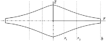
and are thickness and density at = and is the radius of the disk. All other parameters in equation (1) are geometric parameters.The solid disk considered is divided into three regions – inner plastic region, outer plastic region and elastic region. For each region the yield condition will vary. In figure 1,
Elastic-Plastic Deformation of a Rotating Solid
Disk of Exponentially Varying Thickness and
Exponentially Varying Density
Manoj Sahni and Sanjeev Sharma
and
are the interface radii separating the two plastic regions (inner and outer) and the outer elastic region, respectively.Figure 1: Solid disk showing the interface radii.
The plastic (inner region) deformation of the solid disk is governed by the yield condition
= = .
(2)
The equations of equilibrium are all satisfied except,
− ℎ+ ℎ= 0, (3) where h is the thickness function, ρ is the density function and ω is the angular velocity.
Substituting equations (1) and (2) in equation (3) and integrating, one gets
( )
e
( )M
( )
r
e
A
T
T
rr=
θθ=
1 nrbk−
ρ
0ω
2 nrbk 1(4) where,
! = " #
$
$%
.
(5) The linear strain hardening law for a linear isotropic hardening material is
= &1 + ()*+, (6)
where is the initial tensile yield stress, η is the linear strain hardening parameter and
)* is the equivalent plastic strain. Using the equivalence of increment of plastic work,p p
rr r zz eq
T de
θθ θ+
T de
=
T de
(7)
together with the yield condition, leads to
(
0)
1
1 .
p p
eq r zz
e
=
e
θ+
e
=
η
T
T
−
(8) Considering the increment of plastic work, the elastic and plastic strains are added and after the integration, the radial displacement is obtained as
( )
(
)
( )
20 0
2 1
1
1
.
2
r
zz
A
r
u r
T
d
T
E
r
r
ν
ξ ξ ξ
η
η
−
=
+
−
+
∫
(9)
It is observed that
( )
0 0
1
lim
r
zz
r→
r
T
ξ ξ ξ
d
=
∫
( )
[ ]
( )
0
0 0
lim
lim
.
0,
r
zz
zz
r r
d
T
d
dr
r T
r
d
r
dr
ξ ξ ξ
→ →
=
=
∫
(10)
where is finite at the axis. The displacement at r = 0 vanishes and hence the integration constant ,= 0. Substituting = into equation (9) from equation (4), the displacement becomes
( )
(
)
( )
( )
2 0 1
2 3
0
2 1 1
, 2
A r
u r M r M r
T E r r
ν
ρ ω
η
η
−
= + − −
(11)
where,
( )
20 k
r n b
M
r
e
d
ξ
ξ ξ
−
=
∫
,
( )
3
0 0
.
k k t
a
r n a n m
b b b
M r
e
e
e
d
ada
ξ ξ
ξ ξ
− −
=
∫
∫
(12)
The plastic strain components are obtained by subtracting their elastic parts from their total strains as
1
p
rr
u
e T
r E
θ
ν
−
= −
,
0
1
1
1
1
p
r rr rr
du
u
e
T
T
dr
E
T
E
r
ν
ν
η
η
−
−
=
−
=
+
− −
0
1
1 .
p zz
z
T e
T
η
= − −
(13)
Here, the elastic parts of the strains are expressed by stresses with the help of Hooke’s law and the plastic parts with the help of the hardening law.
In the outer plastic region ≤ ≤ the largest stress is equal to the yield stress , i.e. = . Considering the increment of plastic work gives )*= . together with the yield condition one obtains .= −. and .= 0. Since the radial strain is purely elastic and
/.= 1 (⁄
⁄− 1, the strain-displacement relations lead to
0 2
1
1
rr
T
u
T
T
r
E W
θθν
H
=
−
−
and
(
)
1
,
rrdu
T
T
dr
=
E
−
ν
θθ(14)
where
1 =
234 is the normalized hardening parameter and
5
=
6(
) (
)
( )
( )
2 2
0
2
2 2 2 2
1
1
rr
u r
u r
N T
EN
T
r
N
I
N
N
ν
ν
ν
ν
′
=
+
+
−
−
(15)
(
) (
)
( )
( )
2 2 02 2 2 2
1
1
u r
N T
EN
T
u r
r
I
N
N
θθ
ν
ν
ν
′
=
+
+
−
−
(16)
in which a prime denotes differentiation with respect to ‘r’. Substituting equations (15) and (16) in the equation of equilibrium, we have(
)
2
2 2 2
2
2
2 2 2 3 0
0
1
1
1
.
t
k k
k r
m b
d u du
r
r
r
r knr
N
kn
N
u
dr
dr
b
b
N T r
r
kn
N
r e
E
I
b
ν
ν ν
ρ
ν ω
−
+
−
−
+
=
− +
−
−
(17)
To solve this differential equation, let us introduce a new variable 9 = : ⁄ ; and the transformation u(r) = ry(z). Substitution of these in equation (17) gives a differential equation in y(z), whose homogeneous part is
(
)
(
)
2
2 2
2 2
2 1 1
1 1 1 0.
d y dy
z z N N y
dz k dz k ν k z
+ + − + − + + − =
(18)
The above equation has a solution in terms of confluent hypergeometric function given as( )
(1 )(
)
(1 )(
)
3 1, ,1 4 1 1 1, 2 1,
N k N k
y z =A z′ − + F a b z +A z′ − − F a −b + −b z
(19)
where ,<= and ,>= are arbitrary constants. Here?
= −
@;+
@;AB,
= 1 −
@;
and
CD, E, F and F (α, β, γ) is the confluent hypergeometric function given as(
)
(
)
(
)
(
)(
)
(
)(
)
2 3
1 1 2
, , 1 ...
1! 1 2! 1 2 3!
x x x x x
x
F x y z z z z
y y y y y y
+ + +
= + + + +
+ + +
(20)
In this confluent hypergeometric function y should not be zero or a negative integer. The general solution of equation (17) can be written as( )
3 1( )
4 1( )
1( )
,
u r
=
A P r
+
A Q r
+
R r
(21)where
G
=
H
C I?
,
, :
J ;K
andL = @C I?− + 1, 2 − , : J ;
K. (22) The term N in equation (21) is the particular solution of equation (17). N can be obtained using the method of variation of parameters as:
( )
( ) ( )
( ) ( )
1 1 1 2 1
,
op op
R r
=
U
r P r
+
U
r Q r
(23)
where,( )
( )
( )
( )
1 1 1 op r op op rQ
f
U
r
d
N
ξ
ξ
ξ
ξ
= −
∫
and
( )
( )
( )
( )
1 1 2 op r op op rP
f
U
r
d
N
ξ
ξ
ξ
ξ
=
∫
(24)
and
5
O. is the Wronskian given by( )
( )
1( )
( )
1( )
1 1 .
op dQ r dP r
N r P r Q r
dr dr
= −
(25)
Here,
( )
2 0(
2 2)
20
1
1 1 .
t
k r
m
op N r b
f r k n N r e
E rI b
σ
ν ν ρ ν ω
− = − + − −
(26)
The radial and circumferential stresses are obtained as( )
(
)
( )
( )
( )
( )
( )
( )
1 1 3 2 2 2 1 1 0 42 2 2
2 2 1 1 2
1
1
1
1
1
rrP r
dP r
A
r
N
dr
Q r
dQ r
N T
EN
T r
A
N
r
N
dr
I
N
R r
dR r
r
N
dr
ν
ν
ν
ν
ν
ν
+
=
+
+
+
−
−
+
+
(27)
( )
(
)
( )
( )
( )
( )
( )
( )
1 1 3 2 2 0 2 2 2 21 1 1 1
4
. 1
1
P r dP r
A
r dr
N T EN
T r
N
I N Q r dQ r R r dR r
A
r dr r dr
θθ
ν
ν
ν
ν
ν
+ + = + − − + + + (28)
The plastic strain components for this region are given as
.= 0
,
.= PQQ3 − 1R 2,
.= − 2 PQQ3 − 1R.(29)
In an elastic region≤ ≤ , the stress-displacement relations are
(
)
( )
( )
2 1 rr u r ET u r
r
ν
ν
′ = + − and
(
)
( )
( )
2 . 1 u r ET u r
r θθ
ν
ν
′ = + − (30)Substitution of equations (30) in equation (3), we get a differential equation as
t b r m k k
e
r
E
u
b
r
kn
b
r
knr
r
dr
du
dr
u
d
r
−−
−
=
+
−
−
+
2 30 2 2
2
2
1
ν
1
ν
ρ
ω
(31)
The general solution of this equation is given as( )
5 2( )
6 2( )
2( )
u r
=
A P r
+
A Q r
+
R r
(32)
where,( )
2 2 2
1
, , ,
k
r
P r F a b n
r b
=
( )
− + − =
k
b r n b b
a rF r
Q2 2 2 1,2 2,
(33)
and ?= −;+S; , = 1 −; .The particular solution N is obtained in the form
( )
r U( ) ( )
r P r U( ) ( )
rQ rR2 = 1el 2 + 2el 2
(34)
where,
( )
( )
( )
( )
22 1
el r
el
el r
Q
f
U
r
d
N
ξ
ξ
ξ
ξ
= −
∫
and
( )
( )
( )
( )
2 2 2
el r
el
el r
P
f
U
r
d
N
ξ
ξ
ξ
ξ
=
∫
(35)
and 5)Tis the Wronskian given by
( )
( )
2( )
( )
2( )
2 2
el dQ r dP r
N r P r Q r
dr dr
= −
and
( )
(
)
( )E
e
r
r
f
t
b r m el
−
−
−
=
2 2
0
1
ν
ω
ρ
(36)
The radial and circumferential stresses are
( )
( )
( )
( )
( )
( )
( )
2 2 2
5 2
2 2 2
6
1
rr
P r dP r R r
A
r dr r
E
T r
Q r dQ r dR r
A
r dr dr
ν
ν
ν
ν
+ + +
=
−
+ +
(37)
( )
( )
( )
( )
( )
( )
( )
2 2 2
5 2
2 2 2
6
.
1
P r
dP r
R r
A
r
dr
r
E
T
r
Q r
dQ r
dR r
A
r
dr
dr
θθ
ν
ν
ν
ν
+
+
+
=
−
+
+
(38)
III. DETERMINATIONOFINTEGRATION
CONSTANTSANDNUMERICALDISCUSSIONS
The expressions for stresses and displacement for different regions of deformation contain the unknown integration constants ,, ,<, ,>, ,U, ,Vand the interface radii and . For the determination of these seven unknowns there are seven nonredundant conditions available:
,
and u are individually continuous at and , and vanishes at the outer boundary of the disk, i.e. at r = b. These conditions are written explicitly as( )
1( )
1,
ip op
u
r
=
u
r
ip( )
1 op( )
1,
rr rr
T
r
=
T
r
T
ip( )
r
1T
op( )
r
1,
θθ
=
θθ( )
2( )
2,
op el
u
r
=
u
r
( )
2( )
2,
op el
rr rr
T
r
=
T
r
T
θθop( )
r
2=
T
θθel( )
r
2,
( )
0.
elrr
T
b
=
When n and m vanishes, the solution describes the behaviour of a rotating solid disk with uniform thickness
and uniform density.
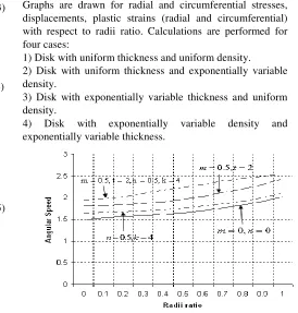
Graphs are drawn for radial and circumferential stresses, displacements, plastic strains (radial and circumferential) with respect to radii ratio. Calculations are performed for four cases:
1) Disk with uniform thickness and uniform density. 2) Disk with uniform thickness and exponentially variable density.
3) Disk with exponentially variable thickness and uniform density.
[image:4.595.284.558.76.363.2]4) Disk with exponentially variable density and exponentially variable thickness.
Figure 2: Angular speed against radii ratio.
In figure 2, it can seen that for the disk with uniform thickness and uniform density with linear strain hardening parameter I = 1/3, angular speed required for initial yielding and fully plasticity is 1.48735 and 2.01571 respectively. The results obtained by Gamer [5] are Ω= 1.54919 and
Ω= 2.08043 for I = 0.5. The variation between the results is because of consideration of different hardening parameter, while the trends of graphs are same. For a disk with exponentially variable thickness (n = 0.5, k = 4), the angular speed is 1.63452 and 2.10301 for initial yielding and fully plasticity respectively. For the case with uniform thickness and exponentially varying density (m = 0.5, t = 2), angular speed required for initial yielding and fully plasticity are 1.8153 and 2.44011, which is very high as compared to the disk with uniform thickness and uniform density. For a disk with exponentially varying thickness and exponentially varying density (m = 0.5, t = 2, n = 0.5, k = 4), angular speed required for initial yielding and fully plasticity is 1.94985 and 2.53629 which is higher as compared to other density and thickness parameters.
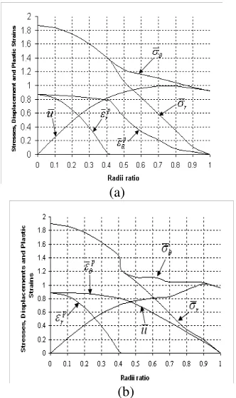
Further the stresses, displacement and plastic strains are calculated for the partially plastic case with hardening parameter I = 1/3 and outer radii as X = 0.5. These are depicted in figure 3 for (a) uniform thickness-variable density, and (b) variable thickness-variable density disk. The integration constants in non-dimensional form for uniform thickness and variable density are calculated as ,YYY = Z[
3 =
1.16683, ,YYY =< Z_
J[`H= 0.0828, ,YYY => JZ[bHa = 0.00870242 ,
,U
YYY = ,U= 0.593503 , ,YYY =V Zg
plastic region and corresponding angular velocity Ω=1.96853. Similarly, the integration constants are calculated for variable thickness-variable density disk. In non-dimensional form these are ,YYY = 1.18352 , ,YYY =<
−0.0258557, ,YYY = 0.564171> , ,YYY = 0.0414589U , ,YYY =V
0.578308 with interface radii X = 0.224057 and corresponding angular velocity is Ω=2.07676.
Stresses, displacements and plastic strains are drawn in figure 3 for uniform thickness-variable density disk and variable thickness–variable density disk. It is seen from figure 3 that radial and circumferential stresses are maximum at the internal surface and observed that upto the inner plastic region; stresses are same and thereafter-radial stress decreases faster radially than that of circumferential stress. It has also been observed that a plastic strain vanishes at the interface radii. From figure 3, it has been observed that circumferential stress is maximum for the disk whose thickness is constant and density varies exponentially as compared to the disk whose thickness and density varies exponentially.
(a)
(b)
Figure 3: Normalized Stresses and displacement for partially plastic case with (a) uniform thickness –
variable density disk (m = 0.5, t = 2) and (b) variable thickness - variable density disk
(n = 0.5, k = 4, m = 0.5, t = 2).
The results for the fully plastic case are obtained using continuity and boundary conditions as
( )
r1 u( )
r1uip = op
,
( )
r1( )
r1op r ip
r σ
σ =
,
( )
r1( )
r1op ip
θ
θ σ
σ =
,
σrop( )
b =0(a)
[image:5.595.342.508.49.328.2]
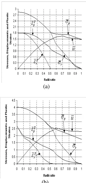
(b)
Figure 4: Normalized Stresses and displacement for fully plastic case with (a) uniform thickness – variable density disk (m = 0.5, t = 2) and (b) variable thickness - variable
density disk (n = 0.5, k = 4, m = 0.5, t = 2).
In the fully plastic case outer interface radii reaches the boundary, i.e. X = 1.0 .For the disk with uniform thickness and variable density, the integration constants in non-dimensional are ,YYY = 1.86626 , ,YYY = 0.584531< , ,YYY =>
0.11508 with interface radii X = 0.421878 and corresponding angular velocity is Ω= 2.44011
,
while for the disk with variable thickness and variable density, the integration constants are ,YYY = 1.89832 , ,YYY = 0.0271469< ,,>
YYY = 1.24442 with interface radii X= 0.414895 and corresponding angular velocity is Ω
=
2.53629. Stresses, displacement and plastic strains are plotted against radii ratio in figure 4. It has been observed from figure 4 that plastic strains are high at the internal surface and vanishes at the interface radii. In addition, circumferential and radial stresses are maximum at the internal surface. [image:5.595.79.245.326.630.2]
(a)
[image:6.595.91.237.48.356.2]
(b)
Figure 5: Normalized Stresses and displacement beyond fully plastic state, h > jk for H = 1/3, m = 0.5, t = 2,
n = 0.5, k = 4 for (a) Ω = 3.0 and (b) Ω = 3.5
The integration constants for the angular speed Ω = 3.0 >
Ω are ,YYY = 2.85468 , ,YYY = 0.205793< , ,YYY = 2.08678>
with interface radii X= 0.514423, while for the disk with angular speed Ω = 3.5 > Ω
,
the integration constants are,
YYY = 4.02113, ,YYY = 0.479066< , ,YYY = 3.09293>
,
with interface radii X = 0.571153. The stresses, displacement and plastic strains for two angular speeds greater than the fully plastic limit are drawn in figure 5. It has been observed from figure 5 that with the increase in angular speed beyond the fully plastic limit, all parameters shows a significant change. From figures 3 and 4, it has also been observed that the magnitudes of the plastic strains are sufficiently small which justifies the assumption of the small deformation theory.IVCONCLUSION
An analytical solution is obtained for elastic-plastic deformations of linear strain hardening solid disk of exponentially variable thickness and exponentially variable density. The results of uniform thickness and uniform density are verified with those available in literature. It has been observed that for exponentially variable thickness and exponentially variable density high angular speed is required for a material to yield and then becomes plastic as compared to the disk with other parameters, which in turns give more significant and economic design by an appropriate choice of thickness and density parameters.
REFERENCES
[1] S. P. Timoshenko and J. N. Goodier, “Theory of Elasticity”, 3rd Ed.,
McGraw Hill, 1970.
[2] S. C. Ugural and S. K. Fenster, “Advanced Strength and Applied Elasticity”, Elsevier, 1987.
[3] F. Laszlo, “Geschleuderte udrehungskorper im Gebiet bleibender Deformation”, ZAMM, pp. 281–293, 1925.
[4] U. Gamer, “Tresca’s Yield Condition and the Rotating Solid Disk”, J. Appl. Mech., vol. 50, pp. 676-678, 1983.
[5] U. Gamer, “Elastic-Plastic Deformation of the Rotating Solid Disk”, Ingenieur Archiv, vol. 54, pp. 345-354, 1984.
[6] U. Guven, “On the Stresses in an Elastic–Plastic Annular Disk of Variable Thickness under External Pressure”, Int. J. Solid Structures, vol. 30, pp. 651–658, 1993.
[7] U. Guven, “On the Applicability of Tresca’s Yield Condition to the Linear Hardening Rotating Solid Disk of Variable Thickness”, ZAMM, vol. 75, pp. 397 – 398, 1995.
[8] Y. Orcan and A. N. Eraslan, “Elastic-Plastic Deformation of a Rotating Solid Disk of Exponentially Varying Thickness”, Mechanics of Materials, vol. 34, pp. 423-432, 2002.
[9] L. H. You, S. Y. Long and J. J. Zhang, “Perturbation Solution of Rotating Solid Disks with Nonlinear Strain Hardening”, Mech. Res. Comm., vol. 24, pp. 649-658, 1997.
[10] A. N. Eraslan, “Inelastic Deformations of Rotating Variable Thickness Solid Disks by Tresca and von-Mises Criterion”, Int. J. Comp. Eng. Sci., vol. 3, pp. 89-101, 2002.
[11] A. N. Eraslan, “Stress Distributions in Elastic-Plastic Rotating Disks with Elliptical Thickness Profiles using Tresca and von-Mises Criterion”, ZAMM, vol. 85, Issue 4, pp. 252-266, 2005.
[12] A. M. Zenkour, “Analytical Solutions for Rotating Exponentially-Graded Annular Disks with Various Boundary Conditions”, Int. J. Str. Stab. Dyn., vol. 5, pp. 557-577, 2005.
[13] M. H. Hojjati and S. Jafari, “Semi-exact Solution of Elastic non-uniform Thickness and Density Rotating Disks by Homotopy Perturbation and Adomain’s Decomposition Methods, Part 1 – Elastic Solution”, International Journal of Pressure Vessels and Piping, vol. 85, Issue 12, pp. 871-878, 2008.
[14] M. Sahni and M. Tomar, “Functionally Graded Axisymmetric Rotating Annular Disc with Internal and External Pressure and Constant Poisson’s Ratio”, International Conference on Chemical, Metallurgical and Civil Engineering (ICCMCE; 2015), Singapore, July 9–10, pp. 1-5, 2015.
[15] M. Sahni and R. Sahni, “Rotating Functionally Graded Disc with Variable Thickness Profile and External Pressure”, Elsevier Procedia Computer Science, vol. 57, pp. 1249–1254, 2015.
[16] S. Sharma, P. Thakur and M. Sahni, “Elastic-Plastic Deformation of a Thin Rotating Disk of Exponentially Varying Thickness With Edge Load and Inclusion”, Annals of Faculty Engineering Hunedoara-International Journal of Engineering, pp. 225-232, 2012.
[17] S. Sharma and M. Sahni, “Creep Analysis of Thin Rotating Disc Having Variable Thickness and Variable Density with Edge Loading”, Annals of Faculty Engineering Hunedoara-International Journal of Engineering, pp. 289-296, 2013.
[18] S. Sharma, M. Sahni and Sanehlata, “Elastic-Plastic Transition of Non-Homogeneous Thick-Walled Cylinder under External Pressure”, Applied Mathematical Sciences, vol. 6, pp. 6069–6074, 2012. [19] S. Sharma and M. Sahni, “Thermo Elastic-Plastic Transition of a