Prior selection for panel vector autoregressions

Munich Personal RePEc Archive

Prior selection for panel vector

autoregressions

Korobilis, Dimitris

April 2015

Prior selection for panel vector autoregressions

Dimitris Korobilis University of Glasgow

April 29, 2015

Abstract

There is a vast literature that speci…es Bayesian shrinkage priors for vector autoregressions (VARs) of possibly large dimensions. In this paper I argue that many of these priors are not appropriate for multi-country settings, which motivates me to develop priors for panel VARs (PVARs). The parametric and semi-parametric priors I suggest not only perform valuable shrinkage in large dimensions, but also allow for soft clustering of variables or countries which are homogeneous. I discuss the implications of these new priors for modelling interdependencies and heterogeneities among di¤erent countries in a panel VAR setting. Monte Carlo evidence and an empirical forecasting exercise show clear and important gains of the new priors compared to existing popular priors for VARs and PVARs.

Keywords: Bayesian model selection; shrinkage; spike and slab priors; forecasting;

large vector autoregression

JEL Classi…cation: C11, C33, C52

1

Introduction

Most issues that economists have to deal with when evaluating macroeconomic policies or forecasting economic trends are inherently multivariate, involving analysis of variables such as in‡ation, GDP, the interest rate, and the unemployment rate. Since the seminal paper of Sims (1980), possibly the most popular econometric tool for analyzing multivariate time series data is the vector autoregressive (VAR) model; see Koop and Korobilis (2010) for a recent review of this vast literature. In an increasingly globalized world characterized by a post-…nancial crisis quagmire of elevated economic and political risk for several individual countries (e.g. Iceland’s banking sector collapse) and unions (e.g. the Eurozone debt crisis which peaked in 2010-2012, a¤ecting several countries in the periphery of the European continent), turbulence in global oil markets, and unprecedented exchange rate ‡uctuations, economists are faced with the challenge of having to monitor and model the global rather than the local economy. Such events have given rise to a recent literature which develops econometric methods for panel vector autoregressive (PVAR) models; see Canova and Ciccarelli (2013) for a recent review. PVAR models extend vector autoregressions for macroeconomic variables of a single country, to a setting with many macroeconomic and/or …nancial variables for several countries. This feature allows one to examine interactions, interdependencies, and linkages between di¤erent variables of di¤erent countries. Considering that the VAR has been a powerful tool that allows macroeconomists to link data to economic theories, measure impulse responses, and forecast, the panel VAR can allow us to generalize such useful econometric exercises to the global dimension.

global economy in agony for several years, shows that in a complex, globalized economy the econometrician cannot be certain apriori about the nature of interdependencies that may hold in the data. In extreme cases, for the sake of parsimony and simplicity, many researchers decide to estimate a single VAR for each country, thus, ignoring the possibilities of any linkages between countries1.

The econometric literature has meticulously developed several priors that can impose restrictions on single-country VARs. For example, Banbura et al. (2010) consider VARs with 130 macroeconomic variables for US, leading to more than 200,000 autoregressive coe¢cients to estimate using only 700 monthly time series observations for each variable. Banbura et al. (2010), as well as several other papers such as Carriero, Clark and Marcellino (2011) and Carriero, Kapetanios and Marcellino (2009), rely on the traditional Minnesota prior; see Littermann (1986). Giannone, Lenza and Primiceri (forthcoming) propose a full Bayes treatment of the Minnesota prior by estimating its shrinkage hyperparameter from the likelihood, rather than …ne-tuning it subjectively. George, Sun and Ni (2008) and Korobilis (2008, 2013) develop Bayesian model selection priors which …nd elements of the autoregressive coe¢cients and/or the VAR covariance matrix which are zero; see also Koop (2013) for an application. Villani (2010) and Giannone, Lenza and Primiceri (2014) develop priors for the long-run/steady-state VAR, where both priors have shrinkage properties2_{. One could argue that all these approaches could be readily used in the PVAR}

setting in order to impose restrictions. Nevertheless, all these types of shrinkage priors developed for the VAR model completely ignore the panel dimension of a PVAR and the existence of homogeneities. This means that all the priors above will treat each of theN G with equal weight a-priori, ignoring that there areN copies of the sameGvariables in such a VAR, and that many times macroeconomic and …nancial variables such as GDP, in‡ation, and asset prices for several countries tend to comove.

Following the contribution of Koop and Korobilis (2015), I de…ne parametric and semiparametric Bayesian model selection priors, carefully tailored to incorporate panel restrictions, and in particular I focus on …nding homogeneous coe¢cients and lack of dynamic interdependencies between countries. The set of priors I de…ne have di¤erent properties and a range of trade-o¤s between ‡exibility and computational tractability. Therefore, I implement a detailed Monte Carlo study which allows me to evaluate all priors using arti…cially generated data. Both parametric and semi-parametric priors …nd the correct panel restrictions in sparse PVARs of large dimensions. Additionally, in a forecasting exercise which involves modeling three variables for ten Eurozone countries (i.e. 30-variable panel VAR), I show that the priors proposed in this paper can signi…cantly improve mean and density forecasts compared to the Minnesota prior and an automatic Bayesian model selection prior for VARs, as well as existing competing priors for PVARs. Therefore, the main contribution of this paper is to show that when panel structure is explicit in the data and interdependencies and heterogeneities are present, there is clear theoretical and empirical evidence that the proposed priors will signi…cantly improve inference. This result cannot generalize, of course, to settings without panel structure (e.g. typical VAR for one

1_{A di¤erent extreme case is to allow unrestricted estimation of the large PVAR - such strategy will}

inevitably lead to poor estimates due to the lack of degrees of freedom.

2_{Villani’s (2010) prior is based on a modi…cation of the Minnesota prior, while Giannone, Lenza and}

country), in which case less computationally complex priors such as the Minnesota prior implementation of Giannone, Lenza and Primiceri (forthcoming) are expected to be more e¢cient and possibly more accurate.

In the next section I de…ne the Panel VAR framework and the type of restrictions a researcher is interested in examining. Then in Section 3 I de…ne the parametric and semi-parametric priors and in Section 4 I implement a Monte Carlo exercise where I compare all these priors with typical shrinkage priors for large VARs (without panel structure). In Section 5 I conclude the paper.

2

Vector autoregressions for panels of countries

Letyitdenote a vector ofGdependent variables for countryiobserved at timet,i= 1; ::; N, t= 1; ::; T. The VAR for countryican be written as:

yit=Ai1y1;t 1+:::+Aiiyi;t 1+:::+AiNyN;t 1+"it; (1) where Ai;j are G G matrices for each i; j = 1;2; :::; N, and "it N(0; ii) with ii covariance matrices of dimensionG G. I refer to the collection of suchN country-speci…c VARs, which is of the form

Yt=AYt 1+"t; (2) as a multivariate regression model for the N G 1 vector of endogenous variables Yt =

(y0_1t; ::; y_{N t}0 )0.3 Throughout this paper I assume that "t N(0; ) with a fullN G N G covariance matrix, meaning that cov("it; "jt) = E("it; "jt) = ij 6= 0 where ij is a the ij-thG Gblock of the matrix that denotes the covariance matrix between the errors in the VARs of country iand country j. If no further assumptions are made about the model coe¢cients, I refer to this speci…cation as the unrestricted PVAR.

Just by working with moderate values ofN andG, the dimension of the PVAR will grow quickly and shrinkage may be desirable. For instance, an application of the PVAR method-ology for the currently 19 Eurozone countries using, say, three macroeconomic/…nancial variables for each country, means that the VAR has N G= 57endogenous variables and we have to estimate3249 pautoregressive coe¢cients, for some choice of lag lengthp. Canova and Ciccarelli (2013) and Koop and Korobilis (2015) argue that it is not optimal to treat the PVAR in equation (2) as a large VAR, and shrink uniformly theN G N Gcoe¢cient matrix A. This is because typical shrinkage priors for VARs would ignore the panel structure of the PVAR model. Looking at equation (1) we should expect that lags of own variables for country i have little probability of being zero. In that respect, there is more probability that one or more of the remaining N 1countries’ variables might not be relevant for the equation of country i, that is, one or more of the matrices Ai1; :::; Aii 1; Aii+1; :::; AiN is zero. When such a restriction exists, e.g. Aij = 0, then we say that there are no dynamic interdependencies from country j to country i, i; j = 1; :::; N, i6=j. Similarly, due to the panel structure of the data, we would also expect that some coe¢cients are homogeneous.

3_{For the sake of clarity in my presentation, I don’t introduce exogenous terms or lag lengths higher than}

Koop and Korobilis (2015) note that such cross-sectional homogeneities might exist in the own lags of di¤erent countries, that is, Aii = Ajj, i; j = 1; :::; N, i 6= j. Such a restriction might not shrink parameters to zero, but also saves degrees of freedom and has very important and interesting structural implications (it is a direct test for heterogeneities among countries).

Note that there are N 1 dynamic interdependency restrictions for each country i, meaning that in the PVAR of equation (2) we can impose a maximum of N(N 1) such restrictions. Additionally, according to the de…nition of Koop and Korobilis (2015) we can impose a maximum of N(N₂ 1) cross-sectional homogeneity restrictions. Koop and Korobilis (2015) develop a stochastic search algorithm, that explicitly tests all possible

2N(N 1)dynamic interdependency restrictions, and all the possible2N(N 1)=2cross-sectional homogeneity restrictions4_{. In their application of just 10 Euro-Area countries, the total}

number of restrictions they search using the Gibbs sampler is 290 245 which is a very large number. It is clear that such interdependency and homogeneity restrictions take into account explicitly the panel structure of the VAR.

The Stochastic Search Speci…cation (S4) algorithm of Koop and Korobilis (2015)

builds on the Stochastic Search Variable Selection prior of George and McCullogh (1993) and George et al (2008) for VARs, but it takes into account the panel restrictions described above. The S4 prior for the dynamic interdependency (denoted with the superscript DI) restrictions is

vec(Aij) 1 DIij N 0; 12 I + DIij N 0; 22 I ; (3)

DI

ij Bernoulli DI ; 8 j6=i; (4) where 2₁ is “small” and 2₂ “large” so that, if DI_ij = 0,Aij is shrunk to be near zero and, and if DI_ij = 1, a relatively uninformative prior is used. The S4 prior for the cross-sectional homogeneity (denoted with the superscript CSH) restrictions is

vec(Aii) 1 CSHij N Ajj; ₁2 I + CSHij N Ajj; 2₂ I ; (5) CSH

ij Bernoulli CSH ; 8j6=i; (6) where 2

1 is “small” and 2

2 is “large” so that, if

CSH

ij = 0, Aii is shrunk to be near Ajj, and if CSH_ij = 1, a relatively uninformative prior is used.

While application of the DI restrictions is relatively simple, application of the CSH restrictions is non-trivial. This is because with the CSH prior we seek to test equality of two matrices (Aii=Ajj) and do so for all possible combinations of iand j,i; j= 1; :::; N. The authors provide a novel solution to this sampling problem, and more details can be found in their Appendix. At the same time, there are two important limitations of this prior. First, the kind of restrictions that we want to look at involve matrices withG2elements which are

4_{Note that we can have di¤erent combinations of restrictions holding in a PVAR. For example, for the}

VAR of country iwe can have any one of the dynamic restrictions Aij = 0. However, we can also have

any combinations of two restrictions holding at the same time, e.g. Aij = 0,Ail= 0, for j 6=l. Similar

either zero (Aij = 0) or equal to each other (Aii=Ajj). This prior cannot account for the fact that, say, only some elements ofAiicould be equal to zero. Additionally, because of this group model selection procedure, it is very hard to test the actual restrictions. This would be equivalent to setting 2

1 = 2₁ = 0. However, for computational reasons5 the authors set

> 2₁; 2₁ >0 for some positive being very small but not exactly zero. But that means that the DI and CSH restrictions will only hold approximately, in particular these priors will allow to test the hypothesis Aij 0 and Aii Ajj. In the next Section I motivate model selection priors for PVARs that do not su¤er from these two shortcomings of the S4

prior.

3

Flexible model selection priors

In order to de…ne the relevant priors I propose in this paper, I de…ne an alternative form of the PVAR which is

Yt=Zt +"t; (7)

whereZt=IN G Yt 1, =vec(A0)is theK 1vector of all PVAR coe¢cients,K=N G2.

The models in equations (2) and (7) are observationally equivalent; the di¤erence in their speci…cations serves as a means of using alternative expressions for posterior estimation. Finally, in the hierarchical priors I introduce, some prior hyperparameters have to be selected by the researcher and some prior hyperparameters will have their own priors. I use an underscore in order to distinguish between these two sets of prior hyperparameters, that is, m is a …xed hyperparameter selected by the researcher, andm showing up in a prior is a hyperparameter which is a random variable.

3.1 A parametric PVAR prior

The …rst prior I consider is inspired by Canova and Ciccarelli (2009) who, in the context of time-varying parameter VARs, extract latent factors from the VAR coe¢cients. These factors are lower dimensional representation of the coe¢cient and also serve the purpose of grouping relevant coe¢cients. For example, Canova and Ciccarelli (2009) show that we might want to exatract one factor from each of the G2 coe¢cients of the own lags for each country i - these are the coe¢cients in the matrix Aii in equation (1). Similarly, we can cluster all (N 1)G2 _{in the matrices (A}

i1; :::; Ai;i 1; Ai;i+1; :::; AiN) into a separate factor for each country i. Finally, we can extract a single factor from all K =N G2 coe¢cients. This structure can be represented using the following equation

= +v;

where is a K s matrix of predetermined loadings6, is an s 1 lower dimensional parameter vector (“factors”) with s K, and v N 0; 2I . This hierarchical structure implies that the prior for a is N ; 2_{I , and is indeed a conjugate}

prior since the error variance shows up in the prior variance term.

5_{See also the discussion in George and McCullogh (1997).}

Canova and Ciccarelli (2009) do not consider the possibility that a coe¢cient might be zero, so that their prior can be quite restrictive: it assumes that a single coe¢cient k is always clustered with some other non-zero coe¢cient l, even if the “true” value of k is zero. In order to deal this culprit of the Canova and Ciccarelli (2009) prior, I propose a modi…cation based on spike and slab priors leading to a Bayesian Factor Clustering

and Selection (BFCS)prior which is of the form

k (1 k) 0( ) + k k; (8)

N ; 2I ; (9)

N(0; c) (10)

k Bernoulli( ): (11)

Therefore, with probability1 the coe¢cient k has prior a point mass at zero, denoted using the Dirac delta 0. With probability the same coe¢cient might come from the

clustering/factor structure a-la Canova and Ciccarelli, which is fully described in equation (9).

3.2 A nonparametric PVAR prior

Following ideas from Dunson et al. (2008) we can use in…nite mixtures, by means of Dirichlet process priors, in order to generalize spike and slab priors and at the same time allow for soft clustering of similar coe¢cients. Dunson et al. (2008) and MacLehose et al. (2007) propose the speci…cation

k (1 k) 0( ) + kDP( F0);

where DP( F0) is a Dirichlet process with base measure F0, typically a Gaussian

distribution N(0; c). The formulation above allows a coe¢cient either to shrink to zero or belong in one of many (in…nite) other Gaussian mixture components. Note, however, that all non-zero coe¢cients will be clustered in N(0; c) components. That is, this prior does not allow to obtain more information about common prior locations for homogeneous coe¢cients, and allow sharper posterior inference when the information in the likelihood is weak. To solve this issue, I propose a prior which allows similar coe¢cients to be shrunk to a common prior location, which can be di¤erent for di¤erent groups of similar coe¢cients. In particular, I de…ne the following Bayesian Mixture Shrinkage (BMixS)prior

k N k; 2k ; (12)

k; k2 0( ) 1010 2 + (1 )F (13)

F DP( F0); (14)

F0 N(0; ) Gamma

1 2;

1

2 ; (15)

Beta 1; ' : (16)

Therefore, this prior can achieve shrinkage towards multiple prior locations - one being the point zero which is of interest for model selection, but other locations _k6= 0can exist. The fact that _k2has a Gamma prior7_{implies that it can obtain a range of values that will allow}

to achieve such shrinkage towards the prior location parameter _k. Therefore, this prior is more ‡exible than the Dunson et al. (2008) prior as it can achieve more complex patterns of clustering of relevant parameters. At the same time it can help decrease estimation in the PVAR model by providing more informative prior means and variances.

4

Monte Carlo simulations

In this section I evaluate the ability of the two newly-developed priors to pick up the correct restrictions in PVARs. I compare these priors to unrestricted least squares, two priors for panel vector autoregressions and two popular priors for general vector autoregressions. The PVAR priors are the ones by Koop and Korobilis (2015) and Canova and Ciccareli (2009), both of which are described above in detail.The …rst general VAR prior is the popular Minnesota prior which Banbura, Giannone and Reichlin (2010) and Koop and Korobilis (2013) have used to estimate large VAR systems. The Minnesota prior is based on a shrinkage hyperparameter, which these two studies optimize on a grid based on goodness-of-…t measures8_{. Here I use the algorithm of Giannone, Lenza and Primiceri (forthcoming)}

who develop a full-Bayes approach to estimating the Minnesota shrinkage hyperparameter. The second prior for imposing restrictions on the VAR is the one by George, Sun and Ni (2008). This algorithm is a generalization of the popular Stochastic Search Variable Selection (SSVS) algorithm of George and McCulloch (1993) for univariate regressions. Note that the SSSS of Koop and Korobilis (2015) also builds on the SSVS of George, Sun and Ni (2008). The SSSS algorithm takes into account possible panel restrictions in the VAR and is computationally e¢cient in very high dimensions. In contrast, the SSVS examines all possible2K restrictions in VAR coe¢cients and, as a result, it can only be used in VARs of moderate dimensions. Therefore, we compare the performance of the following priors proposed in this paper:

1. BFCS: Bayesian Factor Clustering and Selection,

2. BMixS: Bayesian Mixture Shrinkage,

with the following priors which are speci…cally developed for PVARs:

3. CC: Factor shrinkage prior of Canova and Ciccareli (2009),

4. SSSS: Stochastic Search Speci…cation Selection prior of Koop and Korobilis (2015),

and, …nally, the following priors which are developed for general large VARs:

7_{In fact, the} 2

k Gamma 1 2;

1

2 induces a heavy-tailed Cauchy prior marginally for coe¢cient k.

8_{Banbura, Giannone and Reichlin (2010) use the MSFE in a training sample in order to select the}

6. SSVS: Stochastic Search Variable Selection as in George, Sun and Ni (2008),

7. GLP: Hierarchical Minnesota prior with data-based estimation of shrinkage factor, as in Giannone, Lenza and Primiceri (forthcoming),

8. OLS: Unrestricted estimator, equivalent to a di¤use prior for VARs; see Kadiyala and Karlsson (1997).

I implement two Monte Carlo experiments: one using a small panel VAR where we impose speci…c interdependency and homogeneity restrictions among di¤erent countries; and one using a larger system with exactly the same VAR structure for each country (full homogeneity imposed). In both experiments I use the same default hyperparameters for all priors (uninformative, where possible). For the BFCS and Canova and Ciccarelli (2009) priors I specify following Canova and Ciccarelli (2013, page 22), and I setc= 4. For the additional hyperaparameter of the BFCS prior I set = 0:5. For the BMixS prior I set

= 4 and '= 1, which are also fairly uninformative choices. For the GLP and S4 _priors

I use the default settings described by the authors. Finally, for the SSVS of George, Sun and Ni (2008) I set 2₁ = 0:0001, 2₂ = 4and = 0:5; see the Technical Appendix for more details. I also simplify estimation by plugging in the OLS estimate of the PVAR covariance matrix, which allows to reduce uncertainty regarding covariance matrix estimates9. This is a typical thing to do in Bayesian analysis of large systems, and has been extensively used in the …rst Bayesian VAR applications of the Minnesota prior; see Kadiyala and Karlsson (1997) for more details and references. In this Monte Carlo exercise interest lies in the large dimensional vector of coe¢cients so I use the OLS estimate of the covariance matrix in order to control for uncertainty regarding (MCMC) sampling of .

Performance of each of the eight estimators/priors is assessed using the Mean Absolute Deviation (MAD). In particular, if _b is an estimate of based on any of the eight priors, and _e is its true value from the DGP, then I de…ne

M AD = 1

K K

X

i=1

jZibi Zieij;

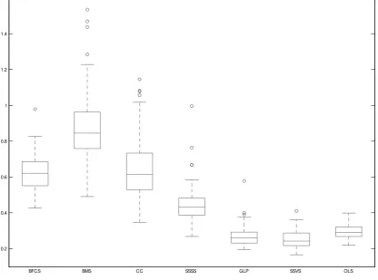
whereK denotes the number of VAR coe¢cients andZi denotes thei-th column ofZ. For each of the exercises below I generateS = 500datasets and, therefore, I calculate500such M AD statistics which I summarize using boxplots.

4.1 Simulation 1: small panel VAR

I generate data from a panel VAR withN = 3countries andG= 2series for each country, p = 1 lags, and T = 50 observations. Therefore, we have 36 autoregressive coe¢cients to estimate with just 50 time series observations. The model I generate has the following

9_{For smaller systems we can simply integrate out the covariance matrix by using a noninformative prior.}

parameters A= 2 6 6 6 6 6 6 4

a1 0 d1 0 e1 0

0 a2 0 d2 0 e2

b1 0 a3 0 d3 0

0 b2 0 a4 0 d4

c1 0 b3 0 a5 0

0 c2 0 b4 0 a6

3 7 7 7 7 7 7 5 ; = 2 6 6 6 6 6 6 4

1 :5 :5 :5 :5 :5

0 1 0 0 0 0

0 0 1 0 0 0

0 0 0 1 0 0

0 0 0 0 1 0

0 0 0 0 0 1

3 7 7 7 7 7 7 5 ;

where ai U(0:5;0:9), bj; dj; ck; ek U( 0:5;0:5), i= 1; :::;6, j = 1; :::;4, k = 1;2, and

= 1 1010. The structure for the VAR coe¢cientsAdoes imply any consistent pattern of cross-sectional homogeneities or absence of dynamic interdependencies. Nevertheless, this speci…c con…guration for the VAR coe¢cients A is used in order to test the general shrinkage performance of the various priors compared in this simulation, regardless of whether heterogeneities and interdependencies occur or not in the (P)VAR model.

Figure 1 presents boxplots of theM AD statistic over the 100 samples. All six Bayesian shrinkage priors (BFCS, BMS, CC, SSSS, GLP and SSVS) introduce some bias in order to achieve a larger reduction in variance, based on the expectation that many coe¢cients are zero. The four panel priors introduce a much larger bias since they incorporate the expectation that groups/clusters of parameters are zero or identical to each other, and their performance is suboptimal, based on theM AD, compared to unrestricted OLS. In fact, the shrinkage GLP and SSVS priors only marginally improve over OLS, showing that in small systems there are no substantial bene…ts from shrinkage.

4.2 Simulation 2: large panel VAR

In the second DGP I consider the case with N = 10,G= 4,p= 1and T = 100. There are 1600 autoregressive coe¢cients to estimate in this model. This model has true parameters

Aij = 0:3 dji jj; d U(0;0:5);

ij =

8 < :

1, ifi=j

0:5, ifi < j

0, ifi > j ;

wherei; j= 1; :::; N G. This DGP does not have an explicit panel structure, but a closer look reveals that several panel restrictions can hold under this form. The VAR coe¢cient matrix A has a form similar to a correlation matrix, where elements which have more distance from the diagonal are essentially zero (thus implying dynamic interdependencies). At the same time, several coe¢cients around the main diagonal, that is, coe¢cients which describe the evolution of the own VAR for each country, will inevitably be similar even when dis generated randomly from a Uniform distribution (thus implying cross-sectional homogeneities). Finally, the factor 0:3 is chosen so as to ensure that the generated PVAR is stationary.

1 0_{The covariance matrix structure is borrowed from the Monte Carlo simulations of George, Sun and Ni}

0.2 0.4 0.6 0.8 1 1.2 1.4 1.6

BFCS BMS CC SSSS GLP SSVS OLS

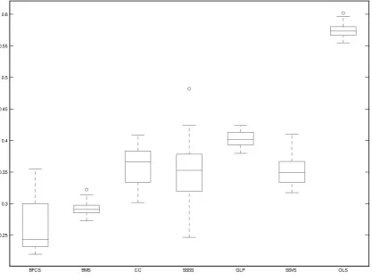
Figure 2 clearly shows that the reduction from the panel VAR priors is substantial. The best performance on average is obtained from the BFCS prior, although the BMS prior has much smaller standard deviation of M ADs over the 100 Monte Carlo samples. The GLP and SSVS priors are also performing. In fact the SSVS turns out to have less uncertainty around posterior estimates compared to the SSSS. This is to be expected given that the SSSS only examines prespeci…ed groups of restrictions, so unless such groupings hold, the SSVS will do better since it examines restrictions on each individual VAR coe¢cient 11_.

The bene…ts of data-based shrinkage plus adding some information about possible grouping of variables results in vast improvements over unrestricted estimation (OLS) and very good improvements compared to typical VAR priors. As a matter of fact, the two panel VAR priors proposed in this paper are by far the best performing when a lare (panel) VAR model has generated our data.

0.25 0.3 0.35 0.4 0.45 0.5 0.55 0.6

BFCS BMS CC SSSS GLP SSVS OLS

Figure 2: Boxplots of MAD statistics in the second Monte Carlo exercise (large VAR model)

1 1_{In that respect, and given the quite similar performance of the two algorithms, the SSSS is to be preferred}

from a computational point of view. In this example with N = 10_, G= 4_{, the algorithm stochastically}

5

Forecasting EuroZone bond yields

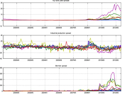
In this Section I present evidence on the ability of the priors suggested in this paper to provide a parsimonious representation of the PVAR, prevent over…tting and give superior forecasts. For this reason, I work with G = 3 monthly variables for N = 10 Eurozone countries for the period 1999M1-2012M12. The series I use are the 10 year bond yields (variable of interest during the EuroZone crisis), total industrial production (a macro fundamental), and the average bid-ask spread (a liquidity measure), for Austria, Belgium, Finland, France, Greece, Ireland, Italy, Netherlands, Portugal and Spain. All series are expressed as spreads from the respective series of Germany. In this exercise the variable of interest is the spread of the 10 year bond yields of each country compared to the yield of the 10 year German bund. These spreads have been the focus of popular press and academic research for the duration of the Eurozone debt crisis.

For the purpose of this paper, a more important aspect is that this dataset is a representative example of panel structure, that is, of possible existence or absence of homogeneities and interdependencies, along with other random groupings between countries. For example, many analysts and policy-makers when looking at these data have been using a grouping between core (Austria, Belgium, Finland, France, Netherlands) and periphery (Greece, Ireland, Italy, Portugal, Spain), in order to show that peripheral countries were exposed to higher sovereign default risk. The kind of comovements in these data can be seen in Figure 3. The priors suggested in this paper could be used to provide a formal data-based grouping of countries and variables, rather than relying on arbitrary groupings. 12

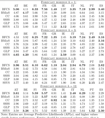
Forecasts are generated iteratively for horizons h = 1; :::;12 and evaluated recursively for the period 2007M1-2012M12, starting with the estimation sample 199M1-2006M12 and adding one observation at a time. Here, I follow Korobilis (2013) and rely on the mean square forecast error (MSFE) and the average predictive likelihood (APL), the former being a measure of accuracy of point forecasts and the latter being a measure of accuracy of the whole predictive distribution (thus, incorporating parameter and estimation uncertainty). Here I consider the exact same priors/estimators I de…ned in the Monte Carlo Section, namely BFCS and BMixS proposed in this paper, the CC and SSSS panel VAR priors, the GLP and SSVS priors for VARs, and …nally the unrestricted OLS estimator (noninformative prior). Note that comparisons should be straightforward and meaningful since all models have exactly the same likelihood, and any di¤erences in posterior predictions are coming from the speci…cation of prior distributions.

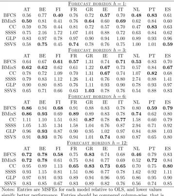
Table 1 presents MSFEs for each of the six priors relative to the MSFE of the OLS. Values lower (higher) than one mean that a method is performing better (worse) compared to OLS. Results are presented for the representative horizons h = 1;3;6;12, in order to evaluate monthly, quarterly, bi-annual and annual forecasts. The results are quite clear and give full support for the following observations

1. All panel priors other than the SSSS (i.e. BFCS, BMix and CC) are consistently better than the Minnesota prior for the VAR.

1 2_{For instance, during the Eurozone crisis, many people have argued that some core countries, such as}

2000M9 2002M5 2004M1 2005M9 2007M5 2009M1 2010M9 2012M5 -10

0 10 20 30

10y bond yield spreads

2000M9 2002M5 2004M1 2005M9 2007M5 2009M1 2010M9 2012M5 -40

-20 0 20 40

Industrial production spread

2000M9 2002M5 2004M1 2005M9 2007M5 2009M1 2010M9 2012M5 0

200 400 600 800

Bid-Ask spread

2. The other VAR prior, the SSVS, seems to be performing relatively well, but it has the lowest MSFEs only in 10% of the cases. Additionally, whenever the SSVS is performing well the BFCS and BMixS priors are very close in terms of performance (only exception is Greece for h= 3). In contrast, in many of the cases that either the BFCS or the BMixS priors are performing well, this performance is far more superior than the SSVS (e.g. Ireland for h = 1). This shows that there is sparsity in the data, which the three model selection priors capture, but at the same time there are homogeneities that the SSVS prior cannot capture (and the two priors suggested in this paper do capture).

Table 1. rMSFEs of Eurozone 10-y bond yield spreads forecasts

Forecast horizon_{h= 1:}

AT BE FI FR GR IE IT NL PT ES

BFCS 0.56 0.77 0.40 0.76 0.72 0.57 0.70 0.48 0.83 0.61 BMixS 0.50 0.81 0.41 0.76 0.64 0.60 0.69 0.62 0.84 0.60 CC 0.59 0.76 0.44 0.81 0.72 0.57 0.70 0.47 0.83 0.63 SSSS 0.75 2.16 1.72 1.07 1.01 0.88 0.72 0.63 0.84 0.62 GLP 0.83 0.97 0.78 0.97 0.90 0.94 1.00 0.89 0.93 0.96 SSVS 0.58 0.75 0.45 0.74 0.78 0.76 0.75 1.00 1.01 0.59

Forecast horizon_{h= 3:}

AT BE FI FR GR IE IT NL PT ES

BFCS 0.64 0.67 0.61 0.57 1.31 0.74 0.71 0.53 0.83 0.70 BMixS 0.62 0.62 0.62 0.61 1.22 0.67 0.73 0.57 0.84 0.67

CC 0.78 0.72 1.09 0.70 1.31 0.67 0.74 1.07 0.82 0.68 SSSS 0.79 0.83 1.12 1.26 1.41 0.76 0.80 2.74 0.88 1.41 GLP 0.90 0.80 0.85 0.76 1.11 0.93 0.90 0.78 0.93 0.97 SSVS 0.65 0.71 0.66 0.63 1.03 0.78 0.76 0.54 0.88 0.83

Forecast horizon_{h= 6:}

AT BE FI FR GR IE IT NL PT ES

BFCS 0.86 0.94 0.68 0.91 0.88 0.83 0.78 0.80 0.59 0.79

BMixS 0.86 0.93 0.69 0.89 0.89 0.83 0.78 0.74 0.62 0.80 CC 1.11 1.10 1.51 0.81 0.87 0.78 0.77 1.58 0.60 0.79 SSSS 1.05 1.35 1.34 1.58 1.04 0.76 0.87 2.94 0.71 0.92 GLP 0.96 0.93 0.87 0.90 0.95 1.02 0.97 0.84 0.88 1.03 SSVS 0.91 0.93 0.76 0.94 1.01 0.74 0.80 0.87 0.65 0.80

Forecast horizon_{h= 12:}

AT BE FI FR GR IE IT NL PT ES

BFCS 0.72 0.78 0.58 0.75 0.83 0.74 0.68 0.46 0.79 0.83 BMixS 0.72 0.78 0.61 0.75 0.84 0.77 0.69 0.52 0.72 0.84 CC 0.95 0.89 1.13 0.65 0.83 0.73 0.65 0.70 0.75 0.80

SSSS 0.93 1.15 0.81 1.51 0.86 0.77 0.78 1.62 0.92 1.11 GLP 0.97 0.91 0.93 0.89 0.94 0.96 0.95 0.86 0.95 0.90 SSVS 0.83 0.85 0.67 0.83 0.89 0.82 0.76 0.56 0.74 0.85 Notes: Entries are MSFEs for each model relative to OLS, and lower values signify better performance. Entries should be compared column-wise, that is, for each country compare the best performing model.

Table 2. APLs of Eurozone 10-y bond yield spreads forecasts

Forecast horizon_{h= 1:}

AT BE FI FR GR IE IT NL PT ES

BFCS 5.06 4.11 6.33 7.56 1.48 2.97 3.35 7.19 2.99 3.40

BMixS 4.87 4.17 5.66 7.10 1.20 3.09 3.01 6.64 2.61 3.15 CC 4.06 3.61 3.90 5.24 1.36 2.42 3.13 4.16 2.45 3.36 SSSS 3.88 4.01 4.50 4.37 1.12 2.68 2.48 4.99 2.54 2.79 GLP 3.75 3.88 4.06 5.47 1.37 2.65 2.53 4.97 2.17 2.81 SSVS 4.72 3.80 5.40 7.11 1.22 3.12 2.80 6.14 2.61 2.80

Forecast horizon_{h= 3:}

AT BE FI FR GR IE IT NL PT ES

BFCS 4.53 3.92 6.25 7.22 1.35 2.45 3.19 7.24 2.49 3.16

BMixS 4.59 3.84 5.87 6.85 1.24 2.50 3.10 6.62 2.40 3.16

CC 3.76 3.24 3.99 5.42 1.33 2.35 2.79 4.85 2.22 3.06 SSSS 3.76 3.30 4.47 4.39 1.17 2.02 2.78 4.67 2.28 2.58 GLP 3.94 3.47 4.55 5.64 1.02 2.39 2.55 5.27 2.17 2.73 SSVS 4.65 4.20 5.86 6.65 1.24 2.59 3.09 6.45 2.27 2.96

Forecast horizon_{h= 6:}

AT BE FI FR GR IE IT NL PT ES

BFCS 3.96 3.51 6.10 6.62 1.18 2.04 2.94 6.79 2.08 2.82

BMixS 3.90 3.42 5.73 6.58 1.04 1.92 2.81 6.54 1.93 2.74 CC 3.22 2.85 3.80 4.81 1.13 1.90 2.55 4.34 1.94 2.64 SSSS 3.04 2.86 4.82 4.12 0.89 1.70 2.20 4.45 1.95 2.65 GLP 3.00 2.64 4.15 5.06 0.85 1.73 2.30 4.75 1.67 2.43 SSVS 3.77 3.40 5.40 6.24 0.97 1.90 2.86 6.20 2.15 2.47

Forecast horizon_{h= 12:}

AT BE FI FR GR IE IT NL PT ES

BFCS 3.61 3.14 5.59 5.57 0.91 1.41 2.48 6.29 1.32 2.29 BMixS 3.59 3.10 5.22 5.57 0.83 1.43 2.35 6.08 1.39 2.17 CC 2.99 2.71 3.52 4.37 0.92 1.36 2.10 4.43 1.35 2.18 SSSS 2.96 2.69 4.27 3.19 0.73 1.31 1.75 4.74 1.57 1.58 GLP 2.78 2.83 3.57 4.43 0.85 1.19 2.02 4.37 1.27 1.93 SSVS 3.58 3.26 4.74 5.52 0.83 1.39 2.16 5.64 1.52 2.30

Note: Entries are Average Predictive Likelihoods (APLs), and higher values signify better performance. Entries should be compared column-wise, that is, for each country compare the best performing model.

6

Conclusions

Given the increased need to model interactions among di¤erent economies or di¤erent …niancial markets (e.g. for stocks, exchange rates, or other assets), panel VARs are meant to become a major tool of empirical analyses and a very natural extension of the benchmark single-country VAR framework. There are, of course, other models for multi-country data such as factor models (Kose, Otrok and Whiteman, 2003) or Global VARs (Dees et al, 2007). However, such alternative methods impose shrinkage by projecting the data into a lower dimensional space. Factor models do this in a data-based way, while GVARs model weakly exogenous variables using weights obtained from billateral trades between the countries involved in the dataset.

References

[1] Banbura, M., Giannone, D., Reichlin, L., 2010. Large Bayesian vector autoregressions.

Journal of Applied Econometrics 25, 71-92.

[2] Canova, F., Ciccarelli, M., 2009. Estimating multicountry VAR models. International Economic Review 50, 929-959.

[3] Canova, F., Ciccarelli, M., 2013. Panel vector autoregressive models: A survey. European Central Bank Working Paper 1507.

[4] Carriero, A., Clark, T., Marcellino, M., 2011. Bayesian VARs: Speci…cation choices and forecast accuracy. Federal Reserve Bank of Cleveland, Working Paper 1112.

[5] Carriero, A., Kapetanios, G., Marcellino, M., 2009. Forecasting exchange rates with a large Bayesian VAR.International Journal of Forecasting 25, 400-417.

[6] Dees, S., Di Mauro, F., Pesaran, M.H., Smith, V., 2007. Exploring the international linkages of the Euro area: A global VAR analysis.Journal of Applied Econometrics 22, 1-38.

[7] Dunson, D. B., Herring, A. H. and Engel, S. M., 2008. Bayesian selection and clustering of polymorphisms in functionally related genes. Journal of the American Statistical Association 103, 534-546.

[8] Gefang, D., 2013. Bayesian doubly adaptive elastic-net Lasso for VAR shrinkage.

International Journal of Forecasting 30,1-11.

[9] Gelman, A., 2006. Prior distributions for variance parameters in hierarchical models.

Bayesian Analysis 1, 515-533.

[10] George, E., McCulloch, R., 1993. Variable selection via Gibbs sampling.Journal of the American Statistical Association 88, 881-889.

[11] George, E., McCulloch, R., 1997. Approaches for Bayesian variable selection.Statistica Sinica 7, 339-373.

[12] George, E., Sun, D., Ni, S., 2008. Bayesian stochastic search for VAR model restrictions.

Journal of Econometrics 142, 553-580.

[13] Giannone, D., Lenza, M., Primiceri, G., 2014. Priors for the long run. manuscript

[14] Giannone, D., Lenza, M., Primiceri, G., forthcoming. Prior selection for vector autoregressions.Review of Economics and Statistics.

[15] Kadiyala, K. R., Karlsson, S., 1997. Numerical methods for estimation and inference in Bayesian VAR-models.Journal of Applied Econometrics, 12, 99-132.

[17] Koop, G., Korobilis, D., 2010. Bayesian multivariate time series methods for empirical macroeconomics. Foundations and Trends in Econometrics 3, 267-358.

[18] Koop, G., Korobilis, D., 2013. Large time-varying parameter VARs. Journal of Econometrics 177, 185-198.

[19] Koop, G., Korobilis, D., 2014. Model uncertainty in panel vector autoregresions.

European Economic Review, revise and resubmit.

[20] Korobilis, D., 2008. Forecasting in vector autoregressions with many predictors.

Advances in Econometrics 23, 403-431.

[21] Korobilis, D., 2013. VAR forecasting using Bayesian variable selection. Journal of Applied Econometrics 28, 204-230.

[22] Kose, M. A., Otrok, C., Whiteman, C. H., 2003. International business cycles: World, region, and country-speci…c factors.American Economic Review 93(4), 1216-1239.

[23] Litterman, R., 1986. Forecasting with Bayesian vector autoregressions – Five years of experience.Journal of Business and Economic Statistics 4, 25-38.

[24] MacLehose, R. F., Dunson, D. B., Herring, A. H. and Hoppin, J. A., 2007. Bayesian methods for highly correlated exposure data.Epidemiology 18, 199-207.

A. Techincal Appendix

Consider the parametrization of the PVAR of the form

Yt=Zt +"t; (A.1) whereZt=IN G Xt,Xt=Yt 1, =vec(A0) is theK 1vector of all PVAR coe¢cients,

K = 1; :::; N G2_{. The parmeter vector of interest is now , but once we know this vector we}

can easily rearrange its elements to construct the original PVAR matrix A.

A.1 Posterior inference in the PVAR using the Bayesian Factor Clustering and Selection (BFCS)

The Bayeian Factor Clustering and Selection prior has the following structure

k (1 k) 0( ) + k k; (A.2)

N ; 2I (A.3)

N(0; cI) (A.4)

k Bernoulli( ); (A.5)

Beta 1; ' : (A.6)

However, this structure implies the following speci…cation for the vector of PVAR coe¢cients

= ( ) +v; (A.7)

where v N 0; 2I and is a K K diagonal matrix with element ii = i, i= 1; :::; K. Here I follow the recommendation of Canova and Ciccarelli (2009) and use the exact decomposition for , observed without error. This is the case where 2 _{= 0.}

Gibbs sampling algorithm for the BMixS algorithm

1. Sample from

( j ) N(E ; V ); (A.8)

where E =V Ze0 _{I e} 1_{Y and V = c} 1_I+Ze0 _{I e} 1_Ze

1

, where Ze=

Z and e = I+ 2_Z0_{Z .}

2. Recover from

( j ) N ( ); 2I : (A.9) 3. Sample _kj _k , where _k denotes the vector with itsk-th element removed, from

and p Yj k; _k; _k = 1 is very costly (see exact equations in Korobilis, 2013), and can also be subject to over‡ow/under‡ow problems. In this case, one can use an approximate algorithm and update all _k at once (not conditional on _k) and calculate l0k N( kj0;1e 8) and l0k N( kj0; c) (1 ), where N(xja; b) denotes the Normal density with meanaand variancebevaluated at the observations x.

4. Sample from

( j ) Beta 1 +X _k; '+X(1 _k) : (A.11)

5. Sample conditional on using standard expressions (see e.g. Koop, 2003).

A.2 Posterior inference in the PVAR using the Bayesian Mixture Shrinkage (BMixS) prior

The Bayesian Mixture Shrinkage (BMixS) prior has the following hierarchical strucure

k N k; 2k ; (A.12)

k; k2 0( ) 1e+10 2 + (1 )F; (A.13)

F DP( F0); (A.14)

F0 N 0; 2 Gamma

1 2;

1

2 ; (A.15)

Beta 1; ' : (A.16)

GivenC mixture components, the equivalent stick breaking representation of this prior is

k N el;e2l ; k= 1; :::; K; l= 1; :::; C ; (A.17)

el;el 2 w0 0( ) 1e+10 2 +

C

X

l=2

wlN 0; 2 Gamma

1 2;

1

2 ; (A.18)

where w0 = and wl = !l

Y

h<l(1 !h) with !l Beta 1; ' , l = 2; :::; C . Here it greatly simpli…es computation if we pre-…x the maximum number of clustersC ; otherwise a Metropolis-Hastings step is required in order to sample the number of cluster con…gurations. We don’t need to be very informative and set C to a very low value (e.g. one or two clusters), but it generally helps ifC K.

Gibbs sampling algorithm for the BMixS algorithm

1. Sample from

2. Sample _el,l= 1; :::; C , from

(_elj ) 0(el); if l= 1

N(E ; V ); otherwise ; (A.20)

where 0(el)is the Dirac delta at zero for parameterel,E =V

XK

j=1;j2l j

2

j ,

and V = 1= 2+XK

j=1;j2l

2

j

1

.

3. Sample_e2_l,l= 1; :::; C , from

e2lj

(

1010(e_l); if l= 1

iGamma 1₂ +nl;1₂ +PCl=2;k2l( k l)2 ; otherwise

; (A.21)

wherenl is the number of coe¢cients (elements) that belong in cluster l.

4. Samplewl from

(wlj ) !l

Y

h<l(1 wh); (A.22) where!l is sampled from

(!lj ) Beta nl+ 1; C

Xl

j=1nj+' : (A.23)

5. Sample conditional on using standard expressions (see e.g. Koop, 2003).

A.3 Posterior inference in the PVAR using the Stochastic Search

Speci…-cation Selection (S4_{) prior of Koop and Korobilis (2015)}

Following the main text, the VAR for country iis

yit=Ai1y1;t 1+:::+Aiiyi;t 1+:::+AiNyN;t 1+"it; (A.24) and the compact form of the PVAR (in matrix form) is

Y =XA+";

where Y = (Y₁0; :::; Y_T0)0, X = (X₁0; :::; X_T0)0 and " = ("0₁; :::; "0_T)0. Note that for notational simplicity I have de…ned Xt = Yt 1, however, the formulae below remain the same if

we generalize to Xt = (I; Yt 1; Yt 2; :::; Yt p; Wt 1; Gt 1) where Wt are country-speci…c exogenous variables and Gtare global exogenous variables.

vec(Aij) 1 DI_ij N 0; 2₁ I_G2 + DI_ij N 0; 2₂ I_G2 ; (A.25)

DI

ij Bernoulli DIij ; 8j6=i; (A.26) DI

ij Beta 1; ' ; (A.27)

while the existence (or absence) of cross-sectional homogeneity can be tested using the prior

vec(Aii) 1 CSHij N Ajj; 2₁ IG2 + CSH_ij N A_jj; 2

2 IG2 ; (A.28)

CSH

ij Bernoulli CSHij ; 8 j6=i; (A.29) CSH

ij Beta 1; ' : (A.30)

We take the hypeparameters with an underscore ('; 2₁; 2₂; 2₁; 2₂) as given, that is, prespeci…ed by the researcher. Additionally, as explained in detail in Koop and Korobilis

(2015) we de…ne a matrix =

N_Y1

i=1

N

Y

j=i+1

i;j, where i;j are K K matrices constructed

using the CSH restriction indicators CSH

ij . First note that CSHij = 0implies that countries iand j have similar coe¢cients (i.e. the homogeneity restrictionAii Ajj holds), and the opposite is true when CSH_ij = 1. The matrix i;j is the identity matrix (i.e. ones on the diagonal zeros elsewhere) with the restriction that itsfi; igdiagonal element is equal to CSH

ij and itsfi; jgnon-diagonal element is equal to 1 CSH_ij . Therefore, each of the possible N(N 1)=2matrices i;j allow us to impose on the PVAR coe¢cients the CSH restriction between countriesiandj, and their product, which is the matrix =

N_Y1

i=1

N

Y

j=i+1

i;j, allows

us to index all 2N(N 1)=2 possible CSH restrictions among the N countries. Therefore, if denotes the posterior mean of the unrestricted vectorized PVAR coe¢cients (i.e. using

a noninformative prior), then _e = =

N_Y1

i=1

N

Y

j=i+1

i;j is simply the K 1 vector of posterior means of the PVAR coe¢cients with the cross-sectional homogeneity restrictions imposed; see Koop and Korobilis (2015) for further details.

Gibbs sampler algorithm for the S4 algorithm

1. Samplevec(A) from

(vec(A)j ) N( ; D ); (A.31) whereD = 1 _X0_X+V0_V 1 _{and =D} 1 _X0_X

OLS , where OLS is the OLS estimate of , andV is a diagonal matrix which has its respective diagonal block of G2 _{elements equal to} 2

1 1 if DIij = 0 or equal to 22 1 if DIij = 1, where

1 _{is aG}2 _{1 vector of ones.}

2. Sample DI_ij from

DI

where !DI_ij = u2;ij

u1;ij+u2;ij with u1;ij = N vec(Aij)j

0_; 2

1IG2 DI_ij and u_2;ij =

N vec(Aij)j0; 22IG2 1 DI

ij , and N(xja; b) denotes the Normal density with mean aand variance bevaluated at the observations x.

3. Sample DI ij from

DI

ij j Beta 1 +

X _DI

ij ; '+

X

1 DI_ij : (A.33)

4. Sample CSH ij from

CSH

ij j Bernoulli !CSHij ; (A.34) where !CSH_ij = v2;ij

v1;ij+v2;ij with v1;ij = N vec(Aii)jvec(Ajj);

2 1IG2

CSH ij and v2;ij =N vec(Aii)jvec(Ajj); 2₂IG2 1 CSH

ij , andN(xja; b)denotes the Normal density with meana and varianceb evaluated at the observations x.

5. Sample CSH ij from

CSH

ij j Beta 1 +

X _CSH

ij ; '+

X

1 CSH_ij : (A.35)

6. Sample conditional onA using standard expressions (see e.g. Koop, 2003).

A.4 Posterior inference in other models examined in this paper

For the SSVS prior for VAR developed by George, Sun and Ni (2008), see the Appendix of their paper. This prior is similar to the S4 _{prior with the exception that it does not}

distinguish between DIs and CSHs, rather it treats restrictions on each VAR coe¢cient uniformly (meaning that each VAR coe¢cient has equal prior weight of importance and only the data will determine which coe¢cients should be shrunk to zero). This prior can be written as

k 1 ij N 0; 21 + ijN 0; 22 ; (A.36)

where in this paper I set ₁ = 0:01 and ₂= 4.

In the case of the Minnesota prior of Giannone et al.(forthcoming) I use the code provided by D. Giannone (http://homepages.ulb.ac.be/~dgiannon/GLPreplicationWeb.zip) and I work with their default settings. Note that this code allows to work only with posterior medians. In order to have better comparability with all other priors in this paper, I allow MCMC updates for this prior in order to account for approximation error when using the Gibbs sampler.