Text Classification from Positive and Unlabeled Data using Misclassified Data Correction

Text Classification from Positive and Unlabeled Data using Misclassified

Data Correction

Fumiyo Fukumoto and Yoshimi Suzuki and Suguru Matsuyoshi

Interdisciplinary Graduate School of Medicine and Engineering University of Yamanashi, Kofu, 400-8511, JAPAN

{fukumoto,ysuzuki,sugurum}@yamanashi.ac.jp

Abstract

This paper addresses the problem of deal-ing with a collection of labeled traindeal-ing documents, especially annotating negative training documents and presents a method of text classification from positive and un-labeled data. We applied an error detec-tion and correcdetec-tion technique to the re-sults of positive and negative documents classified by the Support Vector Machines (SVM). The results using Reuters docu-ments showed that the method was compa-rable to the current state-of-the-art biased-SVM method as the F-score obtained by our method was 0.627 and biased-SVM was 0.614.

1 Introduction

Text classification using machine learning (ML) techniques with a small number of labeled data has become more important with the rapid increase in volume of online documents. Quite a lot of learn-ing techniques e.g., semi-supervised learnlearn-ing, self-training, and active learning have been proposed. Blum et al. proposed a semi-supervised learn-ing approach called the Graph Mincut algorithm which uses a small number of positive and nega-tive examples and assigns values to unlabeled ex-amples in a way that optimizes consistency in a nearest-neighbor sense (Blum et al., 2001). Cabr-era et al. described a method for self-training text categorization using the Web as the corpus (Cabr-era et al., 2009). The method extracts unlabeled documents automatically from the Web and ap-plies an enriched self-training for constructing the classifier.

Several authors have attempted to improve clas-sification accuracy using only positive and unla-beled data (Yu et al., 2002; Ho et al., 2011). Liu et al. proposed a method called biased-SVM that

uses soft-margin SVM as the underlying classi-fiers (Liu et al., 2003). Elkan and Noto proposed a theoretically justified method (Elkan and Noto, 2008). They showed that under the assumption that the labeled documents are selected randomly from the positive documents, a classifier trained on positive and unlabeled documents predicts proba-bilities that differ by only a constant factor from the true conditional probabilities of being positive. They reported that the results were comparable to the current state-of-the-art biased SVM method. The methods of Liu et al. and Elkan et al. model a region containing most of the available positive data. However, these methods are sensitive to the parameter values, especially the small size of la-beled data presents special difficulties in tuning the parameters to produce optimal results.

In this paper, we propose a method for elimi-nating the need for manually collecting training documents, especially annotating negative train-ing documents based on supervised ML tech-niques. Our goal is to eliminate the need for manu-ally collecting training documents, and hopefully achieve classification accuracy from positive and unlabeled data as high as that from labeled posi-tive and labeled negaposi-tive data. Like much previous work on semi-supervised ML, we apply SVM to the positive and unlabeled data, and add the classi-fication results to the training data. The difference is that before adding the classification results, we applied the MisClassified data Detection and Cor-rection (MCDC) technique to the results of SVM learning in order to improve classification accu-racy obtained by the final classifiers.

2 Framework of the System

The MCDC method involves category error cor-rection, i.e., correction of misclassified candidates, while there are several strategies for automati-cally detecting lexical/syntactic errors in corpora (Abney et al., 1999; Eskin, 2000; Dickinson and

training

U

P

P1 _NN₁1

training

SVM

MCDC

N1

RC1

U䠸N1

CP1

CN1

SVM

MCDC

… Final results

SVM

training

selection

classification

P

CP N1

RC1

N1

RC2

N1

CN

MCDC

Figure 1: Overview of the system

Meurers., 2005; Boyd et al., 2008) or categorical data errors (Akoglu et al., 2013). The method first detects error candidates. As error candidates, we focus on support vectors (SVs) extracted from the training documents by SVM. Training by SVM is performed to find the optimal hyperplane consist-ing of SVs, and only the SVs affect the perfor-mance. Thus, if some training document reduces the overall performance of text classification be-cause of an outlier, we can assume that the docu-ment is a SV.

Figure 1 illustrates our system. First, we ran-domly select documents from unlabeled data (U) where the number of documents is equal to that of the initial positive training documents (P1). We set

these selected documents to negative training doc-uments (N1), and apply SVM to learn classifiers.

Next, we apply the MCDC technique to the re-sults of SVM learning. For the result of correction (RC1)1, we train SVM classifiers, and classify the

remaining unlabeled data (U \ N1). For the

re-sult of classification, we randomly select positive (CP1) and negative (CN1) documents classified

by SVM and add to the SVM training data (RC1).

We re-train SVM classifiers with the training doc-uments, and apply the MCDC. The procedure is repeated until there are no unlabeled documents judged to be either positive or negative. Finally, the test data are classified using the final classi-fiers. In the following subsections, we present the MCDC procedure shown in Figure 2. It consists of three steps: extraction of misclassified candi-dates, estimation of error reduction, and correction of misclassified candidates.

1_{The manually annotated positive examples are not}

cor-rected.

Extraction of miss-classified candidates

Training data D

test learning

D䠸SV (Support vectors)

Estimation of error reduction

classification

SV label

䍴

NB label

D䠸Error candidates

Correction of misclassified candidates

D1

D2

Final results Error candidates

SVM NB

Loss function

Judgment using loss values

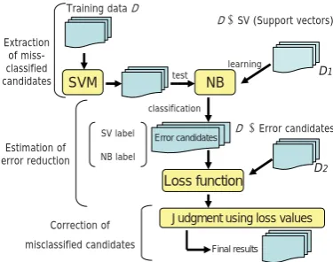
Figure 2: The MCDC procedure

2.1 Extraction of misclassified candidates

Let D be a set of training documents and xk ∈ {x1,x2,· · ·,xm}be a SV of negative or positive

documents obtained by SVM. We remove∪m k=1xk

from the training documents D. The resulting D _{\ ∪}m

k=1xk is used for training Naive Bayes

(NB) (McCallum, 2001), leading to a classifica-tion model. This classificaclassifica-tion model is tested on each xk, and assigns a positive or negative label.

If the label is different from that assigned to xk,

we declarexkan error candidate.

2.2 Estimation of error reduction

We detect misclassified data from the extracted candidates by estimating error reduction. The es-timation of error reduction is often used in ac-tive learning. The earliest work is the method of Roy and McCallum (Roy and McCallum, 2001). They proposed a method that directly optimizes expected future error by log-loss or 0-1 loss, using the entropy of the posterior class distribution on a sample of unlabeled documents. We used their method to detect misclassified data. Specifically, we estimated future error rate by log-loss function. It uses the entropy of the posterior class distribu-tion on a sample of the unlabeled documents. A loss function is defined by Eq (1).

E_Pˆ_D

2∪(xk,yk)

= ₋ 1 |X_|

x∈X

y∈Y

P(y_|x)

×log( ˆPD2∪(xk,yk)(y|x)). (1)

set of test documents. Pˆ_D2∪(xk,yk)(y _| x) shows the learner’s prediction, andD2denotes the

train-ing documents D except for the error candidates

∪l

k=1xk. If the value of Eq (1) is sufficiently

small, the learner’s prediction is close to the true output distribution.

We used bagging to reduce variance ofP(y_|x)

as it is unknown for each test document x. More precisely, from the training documents D, a dif-ferent training set consisting of positive and nega-tive documents is created2. The learner then cre-ates a new classifier from the training documents. The procedure is repeatedmtimes3, and the final class posterior for an instance is taken to be the un-weighted average of the class posteriori for each of the classifiers.

2.3 Correction of misclassified candidates

For each error candidatexk, we calculated the

ex-pected error of the learner, E_Pˆ_D

2∪(xk,yk old) and E_Pˆ_D

2∪(xk,yk new) by using Eq (1). Here, yk old

refers to the original label assigned to xk, and

yk newis the resulting category label estimated by NB classifiers. If the value of the latter is smaller than that of the former, we declare the document xk to be misclassified, i.e., the label yk old is an error, and its true label isyk new. Otherwise, the label ofxkisyk old.

3 Experiments

3.1 Experimental setup

We chose the 1996 Reuters data (Reuters, 2000) for evaluation. After eliminating unlabeled doc-uments, we divided these into three. The data (20,000 documents) extracted from 20 Aug to 19 Sept is used as training data indicating positive and unlabeled documents. We set the range of δ from 0.1 to 0.9 to create a wide range of scenar-ios, whereδrefers to the ratio of documents from the positive class first selected from a fold as the positive set. The rest of the positive and negative documents are used as unlabeled data. We used categories assigned to more than 100 documents in the training data as it is necessary to examine a wide range ofδ values. These categories are 88 in all. The data from 20 Sept to 19 Nov is used

2_{We set the number of negative documents extracted}

ran-domly from the unlabeled documents to the same number of positive training documents.

3_{We set the number ofmto 100 in the experiments.}

as a test set X, to estimate true output distribu-tion. The remaining data consisting 607,259 from 20 Nov 1996 to 19 Aug 1997 is used as a test data for text classification. We obtained a vocabulary of 320,935 unique words after eliminating words which occur only once, stemming by a part-of-speech tagger (Schmid, 1995), and stop word re-moval. The number of categories per documents is 3.21 on average. We used the SVM-Light package (Joachims, 1998)4_{. We used a linear kernel and set} all parameters to their default values.

We compared our method, MCDC with three baselines: (1) SVM, (2) Positive Example-Based Learning (PEBL) proposed by (Yu et al., 2002), and (3) biased-SVM (Liu et al., 2003). We chose PEBL because the convergence procedure is very similar to our framework. Biased-SVM is the state-of-the-art SVM method, and often used for comparison (Elkan and Noto, 2008). To make comparisons fair, all methods were based on a lin-ear kernel. We randomly selected 1,000 positive and 1,000 negative documents classified by SVM and added to the SVM training data in each itera-tion5_{. For biased-SVM, we used training data and} classified test documents directly. We empirically selected values of two parameters, “c” (trade-off between training error and margin) and “j”, i.e., cost (cost-factor, by which training errors on posi-tive examples) that optimized the F-score obtained by classification of test documents.

The positive training data in SVM are assigned to the target category. The negative training data are the remaining data except for the documents that were assigned to the target category, i.e., this is the ideal method as we used all the training data with positive/negative labeled documents. The number of positive training data in other three methods depends on the value of δ, and the rest of the positive and negative documents were used as unlabeled data.

3.2 Text classification

Classification results for 88 categories are shown in Figure 3. Figure 3 shows micro-averaged F-score against the δ value. As expected, the re-sults obtained by SVM were the best among all δ values. However, this is the ideal method that requires 20,000 documents labeled posi-tive/negative, while other methods including our

4

http://svmlight.joachims.org

SVM PEBL Biased-SVM MCDC Level (# of Cat) _{Cat F Cat F (Iter) Cat F (Iter) Cat F (Iter)}

Best GSPO .955 GSPO .802 (26) CCAT .939 GSPO .946 (9) Top (22) Worst GODD .099 GODD .079 (6) GODD .038 GODD .104 (4) Avg .800 .475 (19) .593 .619 (8)

Best M14 .870 E71 .848 (7) M14 .869 M14 .875 (9) Second (32) Worst C16 .297 E14 .161 (14) C16 .148 C16 .150 (3) Avg .667 .383 (22) .588 .593 (7)

Best M141 .878 C174 .792 (27) M141 .887 M141 .885 (8) Third (33) Worst G152 .102 C331 .179 (16) G155 .130 C331 .142 (6) Avg .717 .313 (18) .518 .557 (8)

Fourth (1) – C1511 .738 C1511 .481 (16) C1511 .737 C1511 .719 (4)

Micro Avg F-score .718 .428 (19) .614 .627 (8)

Table 1: Classification performance (δ= 0.7)

0.2 0.3 0.4 0.5 0.6 0.7 0.8

0.1 0.2 0.3 0.4 0.5 0.6 0.7 0.8 0.9

F-score

Delta Value

SVM PEBL Biased-SVM MCDC

Figure 3: F-score against the value ofδ

method used only positive and unlabeled docu-ments. Overall performance obtained by MCDC was better for those obtained by PEBL and biased-SVM methods in allδvalues, especially when the positive set was small, e.g.,δ = 0.3, the improve-ment of MCDC over biased-SVM and PEBL was significant.

Table 1 shows the results obtained by each method with a δ value of 0.7. “Level” indi-cates each level of the hierarchy and the numbers in parentheses refer to the number of categories. “Best” and “Worst” refer to the best and the low-est F-scores in each level of a hierarchy, respec-tively. “Iter” in PEBL indicates the number of it-erations until the number of negative documents is zero in the convergence procedure. Similarly, “Iter” in the MCDC indicates the number of it-erations until no unlabeled documents are judged to be either positive or negative. As can be seen clearly from Table 1, the results with MCDC were better than those obtained by PEBL in each level of the hierarchy. Similarly, the results were

bet-δ SV Ec Err Correct

Prec Rec F 0.3 227,547 54,943 79,329 .693 .649 .670 0.7 141,087 34,944 42,385 .712 .673 .692

Table 2: Miss-classified data correction results

ter than those of biased-SVM except for the fourth level, “C1511”(Annual results). The average num-bers of iterations with MCDC and PEBL were 8 and 19 times, respectively. In biased-SVM, it is necessary to run SVM many times, as we searched “c” and “j”. In contrast, MCDC does not require such parameter tuning.

3.3 Correction of misclassified candidates

Our goal is to achieve classification accuracy from only positive documents and unlabeled data as high as that from labeled positive and negative data. We thus applied a miss-classified data de-tection and correction technique for the classifica-tion results obtained by SVM. Therefore, it is im-portant to examine the accuracy of miss-classified correction. Table 2 shows detection and correction performance against all categories. “SV” shows the total number of SVs in 88 categories in all iter-ations. “Ec” refers to the total number of extracted error candidates. “Err” denotes the number of doc-uments classified incorrectly by SVM and added to the training data, i.e., the number of documents that should be assigned correctly by the correction procedure. “Prec” and “Rec” show the precision and recall of correction, respectively.

corrected. In contrast, there were still other doc-uments that were miss-classified but not extracted as error candidates. We extracted error candidates using the results of SVM and NB classifiers. En-semble of other techniques such as boosting and kNN for further efficacy gains seems promising to try with our method.

4 Conclusion

The research described in this paper involved text classification using positive and unlabeled data. Miss-classified data detection and correction tech-nique was incorporated in the existing classifica-tion technique. The results using the 1996 Reuters corpora showed that the method was comparable to the current state-of-the-art biased-SVM method as the F-score obtained by our method was 0.627 and biased-SVM was 0.614. Future work will in-clude feature reduction and investigation of other classification algorithms to obtain further advan-tages in efficiency and efficacy in manipulating real-world large corpora.

References

S. Abney, R. E. Schapire, and Y. Singer. 1999. Boost-ing Applied to TaggBoost-ing and PP Attachment. In Proc. of the Joint SIGDAT Conference on EMNLP and Very Large Corpora, pages 38–45.

L. Akoglu, H. Tong, J. Vreeken, and C. Faloutsos. 2013. Fast and Reliable Anomaly Detection in Cate-gorical Data. In Proc. of the CIKM, pages 415–424.

A. Blum, J. Lafferty, M. Rwebangira, and R. Reddy. 2001. Learning from Labeled and Unlabeled Data using Graph Mincuts. In Proc. of the 18th ICML, pages 19–26.

A. Boyd, M. Dickinson, and D. Meurers. 2008. On Detecting Errors in Dependency Treebanks. Re-search on Language and Computation, 6(2):113– 137.

R. G. Cabrera, M. M. Gomez, P. Rosso, and L. V. Pineda. 2009. Using the Web as Corpus for Self-Training Text Categorization. Information Re-trieval, 12(3):400–415.

M. Dickinson and W. D. Meurers. 2005. Detecting Errors in Discontinuous Structural Annotation. In Proc. of the ACL’05, pages 322–329.

C. Elkan and K. Noto. 2008. Learning Classifiers from Only Positive and Unlabeled Data. In Proc. of the KDD’08, pages 213–220.

E. Eskin. 2000. Detectiong Errors within a Corpus us-ing Anomaly Detection. In Proc. of the 6th ANLP

Conference and the 1st Meeting of the NAACL, pages 148–153.

C. H. Ho, M. H. Tsai, and C. J. Lin. 2011. Active Learning and Experimental Design with SVMs. In Proc. of the JMLR Workshop on Active Learning and Experimental Design, pages 71–84.

T. Joachims. 1998. SVM Light Support Vector Ma-chine. In Dept. of Computer Science Cornell Uni-versity.

B. Liu, Y. Dai, X. Li, W. S. Lee, and P. S. Yu. 2003. Building Text Classifiers using Positive and Unla-beled Examples. In Proc. of the ICDM’03, pages 179–188.

A. K. McCallum. 2001. Multi-label Text Classifica-tion with a Mixture Model Trained by EM. In Re-vised Version of Paper Appearing in AAAI’99 Work-shop on Text Learning, pages 135–168.

Reuters. 2000. Reuters Corpus Volume1 English Lan-guage. 1996-08-20 to 1997-08-19 Release Date 2000-11-03 Format Version 1.

N. Roy and A. K. McCallum. 2001. Toward Optimal Active Learning through Sampling Estimation of Er-ror Reduction. In Proc. of the 18th ICML, pages 441–448.

H. Schmid. 1995. Improvements in Part-of-Speech Tagging with an Application to German. In Proc. of the EACL SIGDAT Workshop, pages 47–50.