http://www.scirp.org/journal/ajcm
ISSN Online: 2161-1211 ISSN Print: 2161-1203
DOI: 10.4236/ajcm.2019.91001 Feb. 15, 2019 1 American Journal of Computational Mathematics
Comparison of Classical Method, Extension
Principle and
α
-Cuts and Interval Arithmetic
Method in Solving System of Fuzzy Linear
Equations
Sahidul Islam
1, Md. Saiduzzaman
1, Md. Shafiqul Islam
1, Abeda Sultana
21Department of Mathematics, IUBAT (International University of Business Agriculture and Technology), Dhaka, Bangladesh 2Department of Mathematics, Jahangirnagar University, Dhaka, Bangladesh
Abstract
The system of linear equations plays a vital role in real life problems such as optimization, economics, and engineering. The parameters of the system of linear equations are modeled by taking the experimental or observation data. So the parameters of the system actually contain uncertainty rather than the crisp one. The uncertainties may be considered in term of interval or fuzzy numbers. In this paper, a detailed study of three solution techniques namely Classical Method, Extension Principle method and α-cuts and interval Arith-metic Method to solve the system of fuzzy linear equations has been done. Appropriate applications are given to illustrate each technique. Then we dis-cuss the comparison of the different methods numerically and graphically.
Keywords
Fuzzy Set, Classical Solution, Extension Principle,
α-Cut and Interval Arithmetic Method
1. Introduction
There are many linear equation systems in many areas of science and engineer-ing. According to Moore [1], exact numerical data might be unrealistic, but there could be considered uncertain data as more aspects of a real word problem. Fuzzy data are being used as a natural way to describe uncertain data. So, we need to solve those linear systems in which all parameters or some of them are fuzzy numbers. Friedman et al.[2] [3] applied an embedding method for solving
How to cite this paper: Islam, S., Saiduz-zaman, Md., Islam, Md.S. and Sultana, A. (2019) Comparison of Classical Method, Extension Principle and α-Cuts and Inter-val Arithmetic Method in Solving System of Fuzzy Linear Equations. American Journal of Computational Mathematics, 9, 1-24.
https://doi.org/10.4236/ajcm.2019.91001
Received: December 10, 2018 Accepted: February 12, 2019 Published: February 15, 2019
Copyright © 2019 by author(s) and Scientific Research Publishing Inc. This work is licensed under the Creative Commons Attribution-NonCommercial International License (CC BY-NC 4.0). http://creativecommons.org/licenses/by-nc/4.0/
DOI: 10.4236/ajcm.2019.91001 2 American Journal of Computational Mathematics Ax=b, where A is a nonsingular crisp matrix. There are many other numerical
methods for solving fuzzy linear system such as Jacobi, Gauss-Seidel, Adomiam decomposition method and SOR iterative method [4] [5] [6] [7]. Dehgan in [8],
[9] introduced the full fuzzy system in which b and A are fuzzy vector and fuzzy matrix, respectively. Then Kumar in [10] obtained an exact solution of fully fuzzy linear system by solving linear programming.
In 1965, Lotfi A. Zadeh [11], professor of electrical engineering at the Univer-sity of California (Berkley), published the first of his paper on his new theory of Fuzzy Sets and System. After the development of fuzzy set theory, researchers have successfully applied this in economics. Buckley [12] applied fuzzy mathe-matics in finance; in 1992 Buckley devised a technique to solve fuzzy equations in economics and finance. The above methods made us inspired to work on the solution techniques and finally, we got something. The objective of this paper is to present three different and effective methods to solve the system of fuzzy li-near equation. Furthermore, we show the comparison among the methods with the help of numerical calculation as well as graphical representations. The paper organized as follows. In Section 2 we set some basic definitions and notation list. Section 3 deals with the methods. The applications of the models are presented in Section 4 and finally, Section 5 shows the results of the models.
2. Notations and Definitions
2.1. Notations List
A
µ : Membership function of the fuzzy set A. X: Referential set.
I: Valuation set. : Set of real numbers.
X
I : Set of all fuzzy sets from X to I. Aα: α-cut of a fuzzy set A. Aα +: Strong α-cut of a fuzzy set A.
∀: For all.
∃: There exist.
C
A : Complement of a fuzzy set A.
AB: Intersection of two fuzzy sets A and B. AB: Union of two fuzzy sets A and B.
C
X : Classical solution.
e
X : Extension Principle solution.
I
X : α-cut and interval arithmetic solution.
2.2. Fuzzy Sets
A fuzzy set [3]is a class of objects with a continuum of the grade of membership. Let X be a space of points. A fuzzy set A in X is characterized by a membership function which associates with each points in X a real number µA
( )
x in theinterval
[ ]
0,1 with the value of µA at x representing the grade of membershipof x in A. Thus the nearer to the value of µA to unity, the higher the grade of
DOI: 10.4236/ajcm.2019.91001 3 American Journal of Computational Mathematics
2.3. Fuzzy Linear Equation
Fuzzy linear equations are similar to ordinary linear equations in classical ma-thematics. A fuzzy linear equation is of the form A X⋅ =B or A+X =B or
A X⋅ + =C B where A B, and C are given fuzzy numbers and X is an
unknown fuzzy number by which the equation is satisfied.
2.4. The System of Fuzzy Linear Equations
A system of fuzzy linear equations is of the form A X⋅ =B, where A= aij is
a n n× matrix of fuzzy numbers aij,
(
1, 2, ,)
tn
X = x x x is an unknown
1
n× vector of fuzzy numbers xi by which the equation is satisfied and
(
1, 2, ,)
t
n
B = b b b is a n×1 vector of fuzzy numbers bi. Now we can write
corresponding n n× system for all aij∈,1≤i,j≤n as follows:
11 11 11 1 1
21 22 2 2 2
1 2
n
n n nn n n
a a a x b
a a a x b
a a a x b
=
3. Methods
3.1. Classical Solution
We denote the classical solution of A X⋅ =B as Xc, if it exists.
Substitute the α-cuts of aij, xi and bi for aij, xi and bi
(
1≤i j, ≤3)
respectively in the system of linear equations
11 1 12 2 13 3 1,
a x +a x +a x =b (1)
21 1 22 2 23 3 2,
a x +a x +a x =b (2)
31 1 32 2 33 3 3,
a x +a x +a x =b (3)
After substituting the α-cuts of aij, xi and bi for aij , xi and bi
(
1≤i j, ≤3)
in the Equations (1)-(3), we get the following three intervalequa-tions ∀ ∈α
[ ]
0,1 ,( )
( )
( )
( )
( )
( )
( )
( )
( )
( )
( )
( )
( )
( )
11 11 1 1 12 12 2 2
13 13 3 3 1 1
, , , ,
, , ,
L U L U L U L U
L U L U L U
a a x x a a x x
a a x x b b
α
α
α
α
α
α
α
α
α
α
α
α
α
α
⋅ + ⋅
+ ⋅ = (4)
( )
( )
( )
( )
( )
( )
( )
( )
( )
( )
( )
( )
( )
( )
21 21 1 1 22 22 2 2
23 23 3 3 2 2
, , , ,
, , ,
L U L U L U L U
L U L U L U
a a x x a a x x
a a x x b b
α
α
α
α
α
α
α
α
α
α
α
α
α
α
⋅ + ⋅
+ ⋅ = (5)
( )
( )
( )
( )
( )
( )
( )
( )
( )
( )
( )
( )
( )
( )
31 31 1 1 32 32 2 2
33 33 3 3 3 3
, , , ,
, , ,
L U L U L U L U
L U L U L U
a a x x a a x x
a a x x b b
α
α
α
α
α
α
α
α
α
α
α
α
α
α
⋅ + ⋅
+ ⋅ = (6)
We now need to simplify these equations.
Assuming that all the aij and bi are triangular fuzzy numbers and put
1
α = in Equations (4)-(6). Then we obtain the crisp linear system of equations
DOI: 10.4236/ajcm.2019.91001 4 American Journal of Computational Mathematics 21 1 22 2 23 3 2
a x +a x +a x =b
31 1 32 2 33 3 3 a x +a x +a x =b
The sign of the solutions x x1, 2 and x3 determines the sign of the unknown
fuzzy numbers x x1, 2 and x3. Let us assume for this discussion that all the 0
ij
a > and all the bi>0, so that we try for xi >0,i=1, 2, 3. We get from
Equ-ations (4)-(6)
( )
( )
( )
( )
( )
( )
( )
( )
( )
( )
( )
( )
( )
( )
11 1 11 1 12 2 12 2
13 3 13 3 1 1
, ,
, ,
L L U U L L U U
L L U U L U
a x a x a x a x
a x a x b b
α
α
α
α
α
α
α
α
α
α
α
α
α
α
⋅ ⋅ + ⋅ ⋅
+ ⋅ ⋅ = (7)
( )
( )
( )
( )
( )
( )
( )
( )
( )
( )
( )
( )
( )
( )
21 1 21 1 22 2 22 2
23 3 23 3 2 2
, ,
, ,
L L U U L L U U
L L U U L U
a x a x a x a x
a x a x b b
α
α
α
α
α
α
α
α
α
α
α
α
α
α
⋅ ⋅ + ⋅ ⋅
+ ⋅ ⋅ = (8)
( )
( )
( )
( )
( )
( )
( )
( )
( )
( )
( )
( )
( )
( )
31 1 31 1 32 2 32 2
33 3 33 3 3 3
, ,
, ,
L L U U L L U U
L L U U L U
a x a x a x a x
a x a x b b
α
α
α
α
α
α
α
α
α
α
α
α
α
α
⋅ ⋅ + ⋅ ⋅
+ ⋅ ⋅ = (9)
which yields a 6 6× crisp system of linear equations as below
( )
( )
( )
( )
( )
( )
( )
11L 1L 12L 2L 13L 3L 1L
a α ⋅x α +a α ⋅x α +a α ⋅x α =b α (10)
( )
( )
( )
( )
( )
( )
( )
21L 1L 22L 2L 23L 3L 2L
a α ⋅x α +a α ⋅x α +a α ⋅x α =b α (11)
( )
( )
( )
( )
( )
( )
( )
31L 1L 32L 2L 33L 3L 3L
a α ⋅x α +a α ⋅x α +a α ⋅x α =b α (12)
( )
( )
( )
( )
( )
( )
( )
11U 1U 12U 2U 13U 3U 1U
a α ⋅x α +a α ⋅x α +a α ⋅x α =b α (13)
( )
( )
( )
( )
( )
( )
( )
21U 1U 22U 2U 23U 3U 2U
a α ⋅x α +a α ⋅x α +a α ⋅x α =b α (14)
( )
( )
( )
( )
( )
( )
( )
31U 1U 32U 2U 33U 3U 3U
a α ⋅x α +a α ⋅x α +a α ⋅x α =b α (15)
We solve this system for xiL
( )
α and xiU( )
α ,i=1, 2, 3,α∈[ ]
0,1 .Using matrix notation this system can be written as
( )
( )
( )
( )
( )
( )
( )
( )
( )
( )
( )
( )
( )
( )
( )
( )
( )
( )
( )
( )
( )
( )
( )
( )
( )
( )
( )
( )
( )
( )
11 12 13 1 1
21 22 23 2 2
31 32 33 3 3
11 12 13 1 1
21 22 23 2 2
31 32 33 3 3
0 0 0
0 0 0
0 0 0
0 0 0
0 0 0
0 0 0
L L L L L
L L L L L
L L L L L
U U U U U
U U U U U
U U U U U
a a a x b
a a a x b
a a a x b
a a a x b
a a a x b
a a a x b
α α α α α
α α α α α
α α α α α
α α α α α
α α α α α
α α α α α
⋅ = (16) Using
( )
( )
( )
( )
( )
( )
( )
( )
( )
( )
( )
( )
( )
( )
( )
( )
( )
( )
11 12 13
21 22 23
31 32 33
11 12 13
21 22 23
31 32 33
0 0 0
0 0 0
0 0 0
0 0 0
0 0 0
0 0 0
L L L
L L L
L L L
U U U
U U U
U U U
a a a
a a a
a a a
W
a a a
a a a
a a a
α α α
α α α
α α α
α α α
α α α
α α α
= ,
( )
( )
( )
( )
( )
( )
1 2 3 1 2 3 L L L U U U x x x S x x x α α α α α α = and( )
( )
( )
( )
( )
( )
1 2 3 1 2 3 L L L U U U b b b V b b b α α α α α α = , (17)
we get a crisp system of the form W S⋅ =V .
sys-DOI: 10.4236/ajcm.2019.91001 5 American Journal of Computational Mathematics
tem is invertible ∀ ∈α
[ ]
0,1 .The system (5.2.29) can be partitioned into two system as
( )
( )
( )
( )
( )
( )
( )
( )
( )
( )
( )
( )
( )
( )
( )
11 12 13 1 1
21 22 23 2 2
31 32 33 3 3
L L L L L
L L L L L
L L L L L
a a a x b
a a a x b
a a a x b
α α α α α
α α α α α
α α α α α
⋅ =
and
( )
( )
( )
( )
( )
( )
( )
( )
( )
( )
( )
( )
( )
( )
( )
11 12 13 1 1
21 22 23 2 2
31 32 33 3 3
U U U U U
U U U U U
U U U U U
a a a x b
a a a x b
a a a x b
α α α α α
α α α α α
α α α α α
⋅ =
That is, WL⋅SL =VL and WU⋅SU =VU. The solution of these crisp systems
determines xiL
( )
α and xiU( )
α ,i=1, 2, 3,α∈[ ]
0,1 , which are used torecon-struct the components of 3 1× fuzzy vector X.
After solving for the xiL
( )
α and xiU( )
α ,i=1, 2, 3,α∈[ ]
0,1 we check to seeif the intervals xi = xiL
( )
α ,xiU( )
α , i=1, 2, 3,α∈[ ]
0,1 define continuousfuzzy numbers for i=1, 2. What is needed is:
1)
(
xiL( )
α)
0α
∂
>
∂ ,
2)
(
xiU( )
α)
0α
∂
<
∂ , and
3) xiL
( )
1 ≤xiU( )
1 for i=1, 2, 3 (equality for triangular shaped fuzzynum-bers).
3.2. Extension Principle Solution
We denote the extension principle solution of a system of fuzzy linear equations by Xe and it always exists but may, or may not satisfy the original system of
fuzzy linear equations. That is, A X⋅ e =B may, or may not be true.
Let the components of Xe are x x1, 2 and x3. In this method, we need to
fuzzify the crisp solutions
(
)
(
)
(
)
(
1 22 33 23 32)
12(
33 2 23 3)
13(
32 2 22 3)
111 22 33 32 23 12 21 33 31 23 13 21 32 31 22
b a a a a a a b a b a a b a b
x
a a a a a a a a a a a a a a a
− − − + −
=
− − − + − (18)
(
)
(
)
(
)
(
11 33 2 23 3)
1(
21 33 31 23)
13(
21 3 31 2)
211 22 33 32 23 12 21 33 31 23 13 21 32 31 22
a a b a b b a a a a a a b a b
x
a a a a a a a a a a a a a a a
− − − + −
=
− − − + − (19)
(
)
(
)
(
)
(
11 22 3 32 2)
12(
21 3 31 2)
1(
21 32 31 22)
311 22 33 32 23 12 21 33 31 23 13 21 32 31 22
a a b a b a a b a b b a a a a
x
a a a a a a a a a a a a a a a
− − − + −
=
− − − + − (20)
using the extension principle. Let
(
)
1 11, 12, 13, 21, 22, 23, 31, 32, 33, ,1 2, 3 1 h a a a a a a a a a b b b =x,
(
)
2 11, 12, 13, 21, 22, 23, 31, 32, 33, ,1 2, 3 2 h a a a a a a a a a b b b =x ,
DOI: 10.4236/ajcm.2019.91001 6 American Journal of Computational Mathematics
(
)
3 11, 12, 13, 21, 22, 23, 31, 32, 33, ,1 2, 3 3 h a a a a a a a a a b b b =x .
To obtain the first component x1 in Xe, we substitute
11, 12, 13, 21, 22, 23, 31, 32, 33, ,1 2, 3 a a a a a a a a a b b b
for
11, 12, 13, 21, 22, 23, 31, 32, 33, ,1 2, 3 a a a a a a a a a b b b
in h a1
(
11,a12,a13,a21,a22,a23,a31,a32,a33, ,b b b1 2, 3)
and evaluate using theexten-sion principle.
It should be noted that,
(
)
(
)
(
)
11 22 33 32 23 12 21 33 31 23 13 21 32 31 22 0
a a a a a a a a a a a a a a a
∆ = − − − + − ≠ ,
that is, the determinant of the coefficients matrix must be nonsingular and in-vertible.
Let α-cut of x1 is x1
[ ]
α = x1L( )
α ,x1U( )
α .Then the α-cut of x1 can be written as
( )
{
(
)
[ ]
[ ]
}
1 min 1 11, 12, 13, 21, 22, 23, 31, 32, 33, ,1 2, 3 :
,
L
ij ij j j
x h a a a a a a a a a b b b
a a b b
α
α α
=
∈ ∈
( )
{
(
)
[ ]
[ ]
}
1 max 1 11, 12, 13, 21, 22, 23, 31, 32, 33, ,1 2, 3 :
,
U
ij ij j j
x h a a a a a a a a a b b b
a a b b
α
α α
=
∈ ∈
Or,
( )
(
(
)
)
(
(
)
)
(
(
)
)
[ ]
[ ]
1 22 33 23 32 12 33 2 23 3 13 32 2 22 3 1
11 22 33 32 23 12 21 33 31 23 13 21 32 31 22
min ;
,
L
ij ij j j
b a a a a a a b a b a a b a b
x
a a a a a a a a a a a a a a a
a a b b
α
α α
− − − + −
=
− − − + −
∈ ∈
(21)
( )
(
(
)
)
(
(
)
)
(
(
)
)
[ ]
[ ]
1 22 33 23 32 12 33 2 23 3 13 32 2 22 3 1
11 22 33 32 23 12 21 33 31 23 13 21 32 31 22
max ;
,
U
ij ij j j
b a a a a a a b a b a a b a b
x
a a a a a a a a a a a a a a a
a a b b
α
α α
− − − + −
=
− − − + −
∈ ∈
(22)
for α ∈
[ ]
0,1 and 1≤i j, ≤3.Similarly, α-cut of x2 is x2
[ ]
α = x2L( )
α ,x2U( )
α . Then the α-cut of x2is
( )
(
(
)
)
(
(
)
)
(
(
)
)
[ ]
[ ]
11 33 2 23 3 1 21 33 31 23 13 21 3 31 2 2
11 22 33 32 23 12 21 33 31 23 13 21 32 31 22
min ;
,
L
ij ij j j
a a b a b b a a a a a a b a b
x
a a a a a a a a a a a a a a a
a a b b
α
α α
− − − + −
=
− − − + −
∈ ∈
(23)
( )
(
(
)
)
(
(
)
)
(
(
)
)
[ ]
[ ]
11 33 2 23 3 1 21 33 31 23 13 21 3 31 2 2
11 22 33 32 23 12 21 33 31 23 13 21 32 31 22
max
,
;
U
ij ij j j
a a b a b b a a a a a a b a b
x
a a a a a a a a a a a a a a a
a a b b
α
α α
− − − + −
=
− − − −
∈ ∈
+
DOI: 10.4236/ajcm.2019.91001 7 American Journal of Computational Mathematics
for α ∈
[ ]
0,1 and 1≤i j, ≤3.And the α-cut of x3 is x3
[ ]
α = x3L( )
α ,x3U( )
α . Then the α-cut of x3 is( )
(
(
)
)
(
(
)
)
(
(
)
)
[ ]
[ ]
11 22 3 32 2 12 21 3 31 2 1 21 32 31 22 3
11 22 33 32 23 12 21 33 31 23 13 21 32 31 22
min ;
,
L
ij ij j j
a a b a b a a b a b b a a a a
x
a a a a a a a a a a a a a a a
a a b b
α
α α
− − − + −
=
− − − + −
∈ ∈
(25)
( )
(
(
)
)
(
(
)
)
(
(
)
)
[ ]
[ ]
11 22 3 32 2 12 21 3 31 2 1 21 32 31 22 3
11 22 33 32 23 12 21 33 31 23 13 21 32 31 22
max ;
,
U
ij ij j j
a a b a b a a b a b b a a a a
x
a a a a a a a a a a a a a a a
a a b b
α
α α
− − − + −
=
− − − + −
∈ ∈
(26)
for α ∈
[ ]
0,1 and 1≤i j, ≤3.After solving for the xiL
( )
α and xiU( )
α ,i=1, 2, 3,α∈[ ]
0,1 we check to seeif the intervals xi = xiL
( )
α ,xiU( )
α , i=1, 2, 3,α∈[ ]
0,1 define continuousfuzzy numbers for i=1, 2. What is needed is:
1)
(
xiL( )
α)
0α
∂ >
∂ ,
2)
(
xiU( )
α)
0α
∂ <
∂ , and
3) xiL
( )
1 ≤xiU( )
1 for i=1, 2, 3 (equality for triangular shaped fuzzynum-bers).
Now by setting
1
2
3 e X
x
x
x
=
we can check whether A X⋅ e=B is true or false.
If we set α =1, we get the crisp solution x1 from Equation (21) and Equation
(22); crisp solution x2 from Equation (23) and Equation (24) and crisp
solu-tion x3 from Equation (25) and Equation (26) by assuming all the aij and bj
are triangular shaped fuzzy numbers and xiL
( )
1 =xiU( )
1 =x ii, =1, 2, 3.3.3.
α
-Cuts and Interval Arithmetic
We denote the α-cut and interval arithmetic solution of a system of fuzzy linear equations by XI and it always exists but may, or may not satisfy the original
system of fuzzy linear equations. That is, A X⋅ I =B may, or may not be true.
Let the components of XI are x x1, 2 and x3. In this method, we need to
fuzzify the crisp solutions
(
)
(
)
(
)
(
)
(
)
(
)
1 22 33 23 32 12 33 2 23 3 13 32 2 22 3 1
11 22 33 32 23 12 21 33 31 23 13 21 32 31 22
b a a a a a a b a b a a b a b
x
a a a a a a a a a a a a a a a
− − − + −
=
− − − + − (27)
(
)
(
)
(
)
(
11 33 2 23 3)
1(
21 33 31 23)
13(
21 3 31 2)
211 22 33 32 23 12 21 33 31 23 13 21 32 31 22
a a b a b b a a a a a a b a b
x
a a a a a a a a a a a a a a a
− − − + −
=
− − − + − (28)
(
)
(
)
(
)
(
11 22 3 32 2)
12(
21 3 31 2)
1 21 32(
31 22)
311 22 33 32 23 12 21 33 31 23 13 21 32 31 22
a a b a b a a b a b b a a a a
x
a a a a a a a a a a a a a a a
− − − + −
=
− − − + − (29)
DOI: 10.4236/ajcm.2019.91001 8 American Journal of Computational Mathematics
We substitute the α-cuts of a11,a12,a13,a21,a22,a23,a31,a32,a33, ,b b b1 2, 3 for
11, 12, 13, 21, 22, 23, 31, 32, 33, ,1 2, 3
a a a a a a a a a b b b in Equations (27)-(29) and the
sim-plifying using interval arithmetic we obtain the α-cuts of x x1, 2 and x3.
It should be noted that
(
)
(
)
(
)
11 22 33 32 23 12 21 33 31 23 13 21 32 31 22 0
a a a a a a a a a a a a a a a
∆ = − − − + − ≠ ,
that is, the determinant of the coefficients matrix must be nonsingular and in-vertible.
Let α-cut of x1 is x1
[ ]
α = x1L( )
α ,x1U( )
α .To find the α-cut of x1 we substitute
11, 12, 13, 21, 22, 23, 31, 32, 33, ,1 2, 3 a a a a a a a a a b b b
for a11,a12,a13,a21,a22,a23,a31,a32,a33, ,b b b1 2, 3 in Equation (27). Then we get,
[ ]
[ ]
1[ ]
(
(
22[ ] [ ]
[ ] [ ]
33 23[ ] [ ]
[ ] [ ]
32)
)
12[ ] [ ] [ ]
[ ] [ ] [ ]
(
(
33 2 23[ ] [ ]
[ ] [ ]
3)
)
13[ ] [ ] [ ]
[ ] [ ] [ ]
(
(
32 2 22[ ] [ ]
[ ] [ ]
3)
)
111 22 33 32 23 12 21 33 31 23 13 21 32 31 22
a a a a a a a a a a
a a a a
b b
a a a a a
b b
x
a a a a a a
b
α α α α α α α α α α α α α α α
α
α α α α α α α α α α α α α α α
− − − + −
=
− − − + −
Let us assume that all aij >0 and all the bj >0. Then by simplifying and
using the interval arithmetic we get,
( )
(
(
1 22 33 1 23 32) (
) (
12 33 2 12 23 3) (
) (
13 32 2 13 22 3)
)
111 22 33 11 32 23 12 21 33 12 31 23 13 21 32 13 31 22
L L L U U U L L L U U U L L L U U U
L
U U U L L L U U U L L L U U U L L L
b a a b a a a a b a a b a a b a a b
x
a a a a a a a a a a a a a a a a a a
α = − − − + −
− − − + − (30)
And
( )
(
(
1 22 33 1 23 32) (
) (
12 33 2 12 23 3) (
) (
13 32 2 13 22 3)
)
111 32 23 11 22 33 12 31 23 12 21 33 13 31 22 13 21 32
U U U L L L U U U L L L U U U L L L
U
L L L U U U L L L U U U L L L U U U
b a a b a a a a b a a b a a b a a b
x
a a a a a a a a a a a a a a a a a a
α = − − − + −
− − − + − (31)
Again let α-cut of x2 is x2
[ ]
α = x2L( )
α ,x2U( )
α . To find the α-cut of x2we substtute a11,a12,a13,a21,a22,a23,a31,a32,a33, ,b b b1 2, 3 for
11, 12, 13, 21, 22, 23, 31, 32, 33, ,1 2, 3 a a a a a a a a a b b b
in Equations (28). Then we get,
[ ]
[ ]
11[ ] [ ] [ ]
(
(
[ ] [ ]
33 2 23[ ] [ ]
[ ] [ ]
3)
)
1[ ] [ ] [ ]
[ ] [ ] [ ]
(
(
21 33 31[ ] [ ]
[ ] [ ]
23)
)
13[ ] [ ] [ ]
[ ] [ ] [ ]
(
(
21 3 31[ ] [ ]
[ ] [ ]
2)
)
211 22 33 32 23 12 21 33 31 23 13 21 32 31 22
a a a a a a a a a a
a a a a a a a a a a a a a a a
b b b b b
x α α α α α α α α α α α α α α α α
α α α α α α α α α α α α α α α
− − − + −
=
− − − + −
Let us assume that all aij >0 and all the bj >0. Then by simplifying and
using the interval arithmetic we get,
( )
(
(
11 33 2 11 23 3) (
) (
21 33 1 31 23 1) (
) (
13 21 3 13 31 2)
)
211 22 33 11 32 23 12 21 33 12 31 23 13 21 32 13 31 22
L L L U U U L L L U U U L L L U U U
L
U U U L L L U U U L L L U U U L L L
a a b a a b a a b a a b a a b a a b
x
a a a a a a a a a a a a a a a a a a
α = − − − + −
− − − + − (32)
And
( )
(
(
11 23 3 11 33 2) (
) (
31 23 1 21 33 1) (
) (
13 31 2 13 21 3)
)
211 32 23 11 22 33 12 31 23 12 21 33 13 31 22 13 21 32
U U U L L L U U U L L L U U U L L L
U
L L L U U U L L L U U U L L L U U U
a a b a a b a a b a a b a a b a a b
x
a a a a a a a a a a a a a a a a a a
α = − − − + −
− − − + − (33)
And finally, let α-cut of x3 is x3
[ ]
α = x3L( )
α ,x3U( )
α . To find the α-cutof x3 we substitute a11,a12,a13,a21,a22,a23,a31,a32,a33, ,b b b1 2, 3 for
11, 12, 13, 21, 22, 23, 31, 32, 33, ,1 2, 3 a a a a a a a a a b b b
DOI: 10.4236/ajcm.2019.91001 9 American Journal of Computational Mathematics
[ ]
[ ]
11[ ]
(
(
[ ] [ ]
22[ ] [ ]
3 32[ ] [ ]
[ ] [ ]
2)
)
12[ ] [ ] [ ]
[ ] [ ] [ ]
(
(
21 3 31[ ] [ ]
[ ] [ ]
2)
)
1[ ] [ ] [ ]
[ ] [ ] [ ]
(
(
21 32 31[ ] [ ]
[ ] [ ]
22)
)
311 22 33 32 23 12 21 33 31 23 13 21 32 31 22
a a a a a a a a a a
a a a a a a a a a a a a
b b b b b
a x
a a
α α α α α α α α α α α α α α α
α
α α α α α α α α α α α α α α α
− − − + −
=
− − − + −
Let us assume that all aij >0 and all the bj >0. Then by simplifying and
using the interval arithmetic we get,
( )
(
(
11 22 3 11 32 2) (
) (
12 21 3 12 31 2) (
) (
21 32 1 31 22 1)
)
311 22 33 11 32 23 12 21 33 12 31 23 13 21 32 13 31 22
L L L U U U L L L U U U L L L U U U
L
U U U L L L U U U L L L U U U L L L
a a b a a b a a b a a b a a b a a b
x
a a a a a a a a a a a a a a a a a a
α = − − − + −
− − − + − (34)
And
( )
(
(
11 32 2 11 22 3) (
) (
12 31 2 12 21 3) (
) (
31 22 1 21 32 1)
)
311 32 23 11 22 33 12 31 23 12 21 33 13 31 22 13 21 32
U U U L L L U U U L L L U U U L L L
U
L L L U U U L L L U U U L L L U U U
a a b a a b a a b a a b a a b a a b
x
a a a a a a a a a a a a a a a a a a
α = − − − + −
− − − + − (35)
After solving for the xiL
( )
α and xiU( )
α ,i=1, 2, 3,α∈[ ]
0,1 we check to seeif the intervals xi = xiL
( )
α ,xiU( )
α , i=1, 2, 3,α∈[ ]
0,1 define continuousfuzzy numbers for i=1, 2. What is needed is:
1) α
(
xiL( )
α)
0∂
>
∂ ,
2)
(
xiU( )
α)
0α
∂
<
∂ , and
3) xiL
( )
1 ≤xiU( )
1 for i=1, 2, 3 (equality for triangular shaped fuzzynum-bers).
Now by setting
1
2
3 I
x
X x
x
=
we can check whether A X⋅ I =B is true or false.
If we set α =1, we get the crisp solution x1 from Equation (30) and Equation
(31); crisp solution x2 from Equation (32) and Equation (33) and crisp solution
3
x from Equation (34) and Equation (35) by assuming all the aij and bj are
triangular shaped fuzzy numbers and xiL
( )
1 =xiU( )
1 =x ii, =1, 2, 3.4. Applications
4.1. Classical Method
Consider the system of fuzzy linear equation in matrix form
(
)
(
)
(
)
(
)
(
)
(
)
1
2
3
1 / 2 / 3 0 0 1 / 1 / 2
0 3 / 4 / 5 0 1 / 2 / 3
0 0 6 / 8 / 12 2 / 5 / 8
x
x
x
−
=
We solve this fuzzy matrix equation using the classical method. The above system can be written as
(
)
(
)
(
)
(
)
(
)
(
)
1
2
3
1 / 2 / 3 1 / 1 / 2 3 / 4 / 5 1 / 2 / 3 6 / 8 / 12 2 / 5 / 8
x
x
x
= −
=
=
(36)
Here a11=
(
1 / 2 / 3)
, a22 =(
3 / 4 / 5)
, and a33=(
6 / 8 / 12)
.Also, we have, b1= −
(
1 / 1 / 2)
, b2 =(
1 / 2 / 3)
and b3=(
2 / 5 / 8)
.DOI: 10.4236/ajcm.2019.91001 10 American Journal of Computational Mathematics
[ ]
( )
( )
[
]
11 11L , 11U 1 , 3
a α =a α a α = +α −α ,
[ ]
( )
( )
[
]
22 22L , 22U 3 , 5
a α =a α a α = +α −α ,
[ ]
( )
( )
[
]
33 33L , 33U 6 2 ,12 4 a α =a α a α = + α − α ,
[ ]
( )
( )
[
]
1 1L , 1U 1 2 , 2
b α =b α b α = − + α −α ,
[ ]
( )
( )
[
]
2 2L , 2U 1 , 3
b α =b α a α = +α −α ,
[ ]
( )
( )
[
]
[ ]
3 3L , 3U 2 3 ,8 3 , 0,1
b α =b α a α = + α − α ∀ ∈α .
Now substituting the α-cuts of a11, a22, a33, b1, b2 and b3 for a11, a22,
33
a , b1, b2 and b3 in the system (36) and we get
[
]
( )
( )
[
]
[
]
( )
( )
[
]
[
]
( )
( )
[
]
1 1
2 2
3 3
1 , 3 , 1 2 , 2
3 , 5 , 1 , 3
6 2 ,12 4 , 2 3 ,8 3
L U
L U
L U
x x
x x
x x
α α α α α α
α α α α α α
α α α α α α
+ − = − + −
+ − = + −
+ − = + −
(37)
If we put α =1, we get the crisp solutions x1=1 2, x2 =1 2 and x3=5 8.
So we assume we can get a solution with x1>0,x1
[ ]
1 =3 2, x2 >0,x2[ ]
1 =5 4and x3>0,x3
[ ]
1 =5 8.From Equation (37) we get,
(
) ( ) (
)
( ) (
(
)
)
(
) ( ) (
)
( ) (
(
)
)
(
) ( ) (
)
( ) (
(
)
)
(
) ( ) (
)
( ) (
(
)
)
(
) ( ) (
)
( ) (
(
)
)
(
) ( ) (
)
( ) (
(
)
)
1 1
2 2
3 3
1 1
2 2
3 3
1 2
1 1 2 or
1
1
3 1 or
3
2 3
6 2 2 3 or
6 2
2
3 2 or
3
3
5 3 or
5
8 3
12 4 8 3 or
12 4
L L
L L
L L
U U
L U
U U
x x
x x
x x
x x
x x
x x
α
α α α α
α α
α α α α
α α
α α α α
α α
α α α α
α α
α α α α
α α
α α α α
α
− +
+ = − + =
+
+
+ = + =
+
+
+ = + =
+
−
− = − =
−
−
− = − =
−
−
− = − =
−
(38)
We find that,
( )
(
)
(
)
1 2
3 0 1
L x α
α α
∂
= >
∂ + ;
(
2( )
)
(
)
22 0 1
L x α
α α
∂
= >
∂ + ;
( )
(
)
(
)
3 2
14 0 6 2
L x α
α α
∂ = >
∂ + ;
(
1( )
)
(
)
21 0 3
U x α
α α
∂ = − <
∂ − ;
( )
(
)
(
)
2 2
2 0 5
U
x α
α α
∂
= − <
∂ − ;
(
3( )
)
(
)
24
0 12 4
U x α
α α
∂
= − <
∂ − .
That is x1L
( )
α , x2L( )
α and x3L( )
α are increasing functions of α ∈[ ]
0,1Al-DOI: 10.4236/ajcm.2019.91001 11 American Journal of Computational Mathematics
so x1L
( )
1 =x1U( )
1 , x2L( )
1 =x2U( )
1 and x3L( )
1 =x3U( )
1 .Hence,
[ ]
(
(
)
)
(
(
)
)
1
1 2 2
,
1 3
x α α α
α α
− + −
= + −
,
[ ]
(
)
(
)
(
(
)
)
21 3
,
3 5
x α α α
α α
+ −
= + −
and 3
[ ]
(
(
)
)
(
(
)
)
2 3 8 3
,
6 2 12 4
x α α α
α α
+ −
= + −
defines the α-cuts of three fuzzy numbers
respectively.
Now the support of x1 is
[ ] (
)
(
)
(
(
)
)
1
1 2 0 2 0 2
0 , 1,
1 0 3 0 3
x = − + × − = −
+ −
and
mod-al of x1 is
[ ]
(
)
(
)
(
(
)
)
11 2 1 2 1 1 1 1
1 , ,
1 1 3 1 2 2 2
x = − + × − = =
+ −
;
The support of x2 is
[ ]
(
)
(
)
(
(
)
)
21 0 3 0 1 3
0 , ,
3 0 5 0 3 5
x = + − =
+ −
and modal of x2
is 2
[ ]
(
(
)
)
(
(
)
)
1 1 3 1 1 1 1
1 , ,
3 1 5 1 2 2 2
x = + − = =
+ −
; and
The support of x3 is
[ ]
(
)
(
)
(
(
)
)
3
2 3 0 8 3 0 1 2
0 , ,
6 2 0 12 4 0 3 3
x = + × − × =
+ × − ×
and modal
of x3 is
[ ] (
)
(
)
(
(
)
)
3
2 3 1 8 3 1 5 5 5
1 , ,
6 2 1 12 4 1 8 8 8
x = + × − × = =
+ × − ×
.
Therefore we can say that, the classical solution Xc exists and its
compo-nents are continuous triangular shaped fuzzy numbers
1
1 2 1 / /
2 3
x ≈ −
, 2
1 1 3 / / 3 2 5
x ≈
and 3
1 5 2 / / 3 8 3
x ≈
.
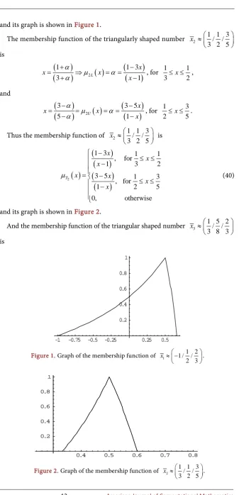
The membership function of the triangularly shaped number 1
1 2 1 / /
2 3
x ≈ −
is
(
)
(
)
1( )
(
(
)
)
1 2 1
1 L 2
x
x x
x
α
µ α
α
− + +
= ⇒ = =
+ − , for
1 1
2
x
− ≤ ≤ ,
and,
(
)
(
)
1( )
(
(
)
)
2 2 3
3 U 1
x
x x
x
α
µ α
α
− −
= = = =
− − , for
1 2
2≤ ≤x 3.
Thus the membership function of 1
1 2 1 / /
2 3
x ≈ −
is
( )
(
)
(
)
(
)
(
)
1
1 1
, for 1
2 2
2 3 1 2
, for
1 2 3
0, otherwise
x
x
x x
x x
x x
µ
+
− ≤ ≤ −
= − ≤ ≤
−
DOI: 10.4236/ajcm.2019.91001 12 American Journal of Computational Mathematics
and its graph is shown in Figure 1.
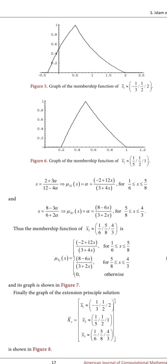
The membership function of the triangularly shaped number 2
1 1 3 / / 3 2 5
x ≈
is
(
)
(
)
2( )
(
(
)
)
1 1 3
3 L 1
x
x x
x
α
µ α
α
+ −
= ⇒ = =
+ − , for
1 1
3≤ ≤x 2,
and
(
)
(
)
2( )
(
(
)
)
3 3 5
5 U 1
x
x x
x
α
µ α
α
− −
= = = =
− − , for
1 3
2≤ ≤x 5.
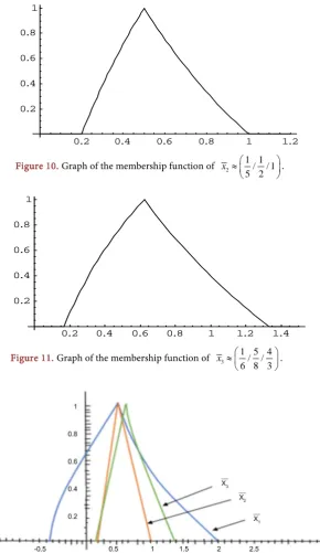
Thus the membership function of 2
1 1 3 / / 3 2 5
x ≈
is
( )
(
)
(
)
(
)
(
)
2
1 3 1 1
, for
1 3 2
3 5 1 3
, for
1 2 5
0, otherwise
x
x
x x
x x
x x
µ
−
≤ ≤ −
= − ≤ ≤
−
(40)
and its graph is shown in Figure 2.
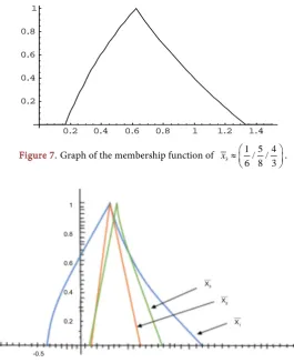
And the membership function of the triangular shaped number 3
1 5 2 / / 3 8 3
x ≈
[image:12.595.207.545.45.745.2]is
Figure 1.Graph of the membership function of 1
1 2 1 / /
2 3
x ≈ −
[image:12.595.207.516.116.335.2] .
Figure 2.Graph of the membership function of 2
1 1 3 / / 3 2 5
x ≈
.
-1 -0.75 -0.5 -0.25 0.25 0.5
0.2 0.4 0.6 0.8 1
0.4 0.5 0.6 0.7 0.8
DOI: 10.4236/ajcm.2019.91001 13 American Journal of Computational Mathematics
(
)
(
)
3( )
(
(
)
)
2 3 2 6
6 2 L 2 3
x
x x
x
α
µ α
α
+ −
= ⇒ = =
+ − , for
1 5
3≤ ≤x 8,
and
(
)
(
)
3( )
(
(
)
)
8 3 8 12
12 4 U 3 4
x
x x
x
α
µ α
α
− −
= = = =
− − , for
5 2
8≤ ≤x 3.
Thus the membership function of 3
1 5 2 / / 3 8 3
x ≈
is
( )
(
)
(
)
(
)
(
)
3
2 6 1 5
, for
2 3 3 8
8 12 5 2
, for
3 4 8 3
0, otherwise
x
x
x x
x x
x x
µ
−
≤ ≤ −
= − ≤ ≤
−
(41)
and its graph is shown in Figure 3.
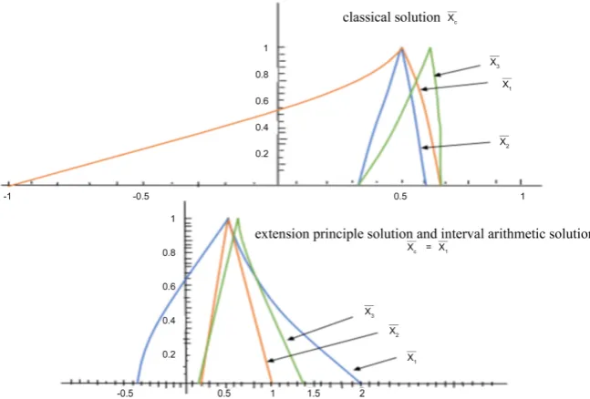
Finally the graph of the classical solution
1
2
3
1 2 1 / /
2 3
1 1 3 / / 3 2 5
1 5 2 / / 3 8 3 c
x
X x
x
≈ −
= ≈
≈
[image:13.595.200.523.69.732.2]is shown in Figure 4.
Figure 3.Graph of the membership function of 3
1 5 2 / / 3 8 3
x ≈
[image:13.595.245.533.578.733.2] .
Figure 4.Graph of the classical solution Xc.
0.3 0.4 0.5 0.6 0.7
DOI: 10.4236/ajcm.2019.91001 14 American Journal of Computational Mathematics
4.2. Extension Principle Method
Consider the system of fuzzy linear equation in matrix form
(
)
(
)
(
)
(
)
(
)
(
)
1
2
3
1 / 2 / 3 0 0 1 / 1 / 2
0 3 / 4 / 5 0 1 / 2 / 3
0 0 6 / 8 / 12 2 / 5 / 8
x
x
x
−
=
We solve this fuzzy matrix equation using the extension principle method. Here, a11=
(
1 / 2 / 3)
, a12 =0, a13=0, a21 =0, a22=(
3 / 4 / 5)
, a23 =0,31 0
a = , a32 =0 and a33=
(
6 / 8 / 12)
. Also, we have, b1= −(
1 / 1 / 2)
,(
)
2 1 / 2 / 3
b = and b3=
(
2 / 5 / 8)
.Then the α-cuts are:
[ ]
( )
( )
[
]
11 11L , 11U 1 , 3
a α =a α a α = +α −α ,
[ ]
( )
( )
[
]
22 22L , 22U 3 , 5
a α =a α a α = +α −α ,
[ ]
( )
( )
[
]
33 33L , 33U 6 2 ,12 4 a α =a α a α = + α − α ,
[ ]
( )
( )
[
]
1 1L , 1U 1 2 , 2
b α =b α b α = − + α −α ,
[ ]
( )
( )
[
]
2 2L , 2U 1 , 3
b α =b α a α = +α −α ,
[ ]
( )
( )
[
]
[ ]
3 3L , 3U 2 3 ,8 3 , 0,1
b α =b α a α = + α − α ∀ ∈α .
Now the crisp solutions are
(
)
(
)
(
)
(
1 22 33 23 32)
12(
33 2 23 3)
13(
32 2 22 3)
22 33 1 111 22 33 32 23 12 21 33 31 23 13 21 32 31 22 11 22 33
b a a a a a a b a b a a b a b a a b
x
a a a a a a a a a a a a a a a a a a
− − − + −
= =
− − − + −
(
)
11 11 12 13 21 22 23 31 32 33 1 2 3 11
, , , , , , , , , , , b
h a a a a a a a a a b b b a
∴ = (42)
(
)
(
)
(
)
(
11 33 2 23 3)
1(
21 33 31 23)
13(
21 3 31 2)
11 33 2 211 22 33 32 23 12 21 33 31 23 13 21 32 31 22 11 22 33
a a b a b b a a a a a a b a b a a b
x
a a a a a a a a a a a a a a a a a a
− − − + −
= =
− − − + −
(
)
22 11 12 13 21 22 23 31 32 33 1 2 3 22
, , , , , , , , , , , b
h a a a a a a a a a b b b a
∴ = (43)
(
)
(
)
(
)
(
11 22 3 32 2)
12(
21 3 31 2)
1(
21 32 31 22)
11 22 3 311 22 33 32 23 12 21 33 31 23 13 21 32 31 22 11 22 33
a a b a b a a b a b b a a a a a a b
x
a a a a a a a a a a a a a a a a a a
− − − + −
= =
− − − + −
(
)
33 11 12 13 21 22 23 31 32 33 1 2 3 33
, , , , , , , , , , , b
h a a a a a a a a a b b b a
∴ = (44)
Since 1 11 b a ,
2
22 b a and
3
33 b
a are increasing functions of b1, b2 and b3; and
decreasing functions of a11, a22 and a33, then
[ ]
[ ]
1( )
( )
1
1 1 11 11
11 11
min : , L
U b b
b b a a
a a
α
α α
α
∈ ∈ =
and 1
[ ]
[ ]
1( )
( )
[ ]
1 1 11 11
11 11
max : , U , 0,1 .
L b b
b b a a
a a
α
α α α
α
∈ ∈ = ∀ ∈