Accepted Manuscript
A new algorithm for prognostics using Subset Simulation
Manuel Chiach´ıo, Juan Chiach´ıo, Shankar Sankararaman,
Kai Goebel, John Andrews
PII:
S0951-8320(16)30733-5
DOI:
10.1016/j.ress.2017.05.042
Reference:
RESS 5862
To appear in:
Reliability Engineering and System Safety
Received date:
7 November 2016
Revised date:
12 May 2017
Accepted date:
27 May 2017
Please cite this article as: Manuel Chiach´ıo, Juan Chiach´ıo, Shankar Sankararaman, Kai Goebel,
John Andrews, A new algorithm for prognostics using Subset Simulation,
Reliability Engineering and
System Safety
(2017), doi:
10.1016/j.ress.2017.05.042
ACCEPTED MANUSCRIPT
ACCEPTED MANUSCRIPT
Highlights
• A new algorithm based on Subset Simulation is provided for general prognostics;
• The Subset Simulation method is used to obtain efficiency for rare events;
• A simulated example and a challenging case study are used to demonstrate its efficacy;
ACCEPTED MANUSCRIPT
A new algorithm for prognostics using Subset Simulation
Manuel Chiach´ıoa,∗, Juan Chiach´ıoa, Shankar Sankararamanb, Kai Goebelc, John Andrewsa
aResilience Engineering Research Group, University of Nottingham, Nottingham, NG7 2RD, UK bSGT Inc., NASA Ames Research Center, Moffett Field, CA 94035-1000
cNASA Ames Research Center, Intelligent Systems Division. Moffett Field, CA 94035-1000
Abstract
This work presents an efficient computational framework for prognostics by combining the particle
filter-based prognostics principles with the technique of Subset Simulation, first developed in S.K. Au and
J.L. Beck [Probabilistic Engrg. Mech., 16 (2001), pp. 263-277], which has been named PFP-SubSim. The idea behind PFP-SubSim algorithm is to split the multi-step-ahead predicted trajectories into multiple
branches of selected samples at various stages of the process, which correspond to increasingly closer
ap-proximations of the critical threshold. Following theoretical development, discussion and an illustrative
example to demonstrate its efficacy, we report on experience using the algorithm for making predictions
for theend-of-life and remaining useful life in the challenging application of fatigue damage propagation
of carbon-fibre composite coupons using structural health monitoring data. Results show that PFP-SubSim
algorithm outperforms the traditional particle filter-based prognostics approach in terms of computational
efficiency, while achieving the same, or better, measure of accuracy in the prognostics estimates. It is also
shown that PFP-SubSim algorithm gets its highest efficiency when dealing with rare-event simulation.
Keywords: Prognostics, rare events, Stochastic modeling, Subset Simulation
1. Introduction
Prognostics is a key technology which allows us to manage assets based on their state of health, as
op-posed to scheduling periodic inspection and maintenance activities based on statistics of mean-time-to-failure
or similar information [1, 2]. In practice, prognostics uses information from health monitoring systems to
determine the state of health of components so as to makeend-of-life(EOL) andremaining useful life(RUL)
predictions based on estimations of the time when specific critical thresholds will be exceeded [3, 4]. The potential of prognostics in positively contributing to safety and asset availability relies in its capacity to
anticipate an anomalous or faulty condition. In particular, one of the challenging problems in prognostics
ACCEPTED MANUSCRIPT
ACCEPTED MANUSCRIPT
can be encountered in practice when predicting the collapse of structures under fatigue degradation,
catas-trophic failures in nuclear plants, run-away conditions in batteries, etc. Due to the lack of data for such
improbable events, model-based instead of data-driven prognostics frameworks have attracted significant
attention in the Prognostic and Health Management (PHM) community for their ability to yield accurate
predictions using a limited amount of data [7]. Model-based prognostics uses the underlying first principles
on which the evolution of the fault indicator is based, thereby reducing thelack of knowledge uncertainty
often present in prognostics [8, 9]. Several examples are found in the literature dealing with model-based
prognostics frameworks for a widespread range of applications, like fatigue damage evolution in engineering
materials [10, 11], failure of electronic components [12], aging of batteries [13, 14], to name but a few.
Be-sides model uncertainty, other important source of uncertainty present in a typical prognostics problem is the uncertainty coming from the use of a specific prognostics algorithm [15]. Sampling-based methods
(e.g. particle filters [PF]) [16, 17] are examples of algorithms used to efficiently approximate the probability
density function (PDF) of the predicted system states through a limited set of discreteparticle paths,
rep-resenting sample trajectories of the system evolution in the state space [18]. Since multi-step ahead state
estimation is required in prognostics [19], then the statistical uncertainty that arises from the
approxima-tion by particles is propagated in time leading to an increase of the final uncertainty for the EOL/RUL
estimation [20]. This drawback can be exacerbated when reaching the failure threshold is a rare event under
the model representing the system evolution, since the referred sample trajectories result in long paths of
predicted states. Higher-density sampling-based methods may be employed achieving higher resolution for
the EOL/RUL predictions, however it is at the expense of a higher computational effort. On the other hand,
choosing a conservative failure threshold might constitute a pragmatic alternative although it results in dis-carding potential useful life. To alleviate this critical issue, some particular solutions have appeared in the
literature to gain prediction accuracy while keeping computational cost at acceptable levels [21–23]. However,
specialized computational frameworks to achieve the required EOL/RUL prediction accuracy still remains
very limited for prognostics involving rare-event simulation.
In this work, a general prognostics algorithm is proposed based on the Subset Simulation method [24].
Sub-set Simulation is an efficient simulation framework which transforms the simulation of a rare-event into the
simulation of a sequence of events of higher probabilities. This general aspect makes Subset Simulation
applicable to a broad range of areas of science and engineering where the simulation of an unlikely event
is required [25, 26]. The pivotal idea behind Subset Simulation in application to prognostics is to split the
multi-step-ahead predicted states of the system into multiple branches of selected samples (“seeds”) at se-lected stages of the process. These seeds provide the starting points for reproducing offsprings of predicted
states, thus leading to a nested sequence of subsets which are adaptively obtained until the failure region is
reached. For the higher subset, all the samples are closely distributed in the vicinity of the final threshold
ACCEPTED MANUSCRIPT
PFP-SubSim and a first version was presented in a conference paper in [27]. The focus here is on
enhance-ments to the methodological aspects behind PFP-SubSim as a general prognostics algorithm. In addition,
insightful examples and extended results are provided.
The paper is organized as follows. Section 2 overviews the mathematical basis and computational aspects
of prognostics. In Section 3, the Subset Simulation method is described and specialized for application to
prognostics, after which the PFP-SubSim algorithm is presented. The efficiency of PFP-SubSim is illustrated
in Section 4 using both a numerical example and also a case study. A discussion about the performance
of PFP-SubSim algorithm in relation to the standard PF-based prognostics algorithm is also provided in
Section 4. Section 5 provides concluding remarks.
2. Foundations of prognostics
Let {xn}n>0 be a Markov process described by the state vector xn taking values in a space denoted
by X ⊂Rnx, and θ ∈ Θ ⊂ Rnθ a set of uncertain model parameters. Let us define an augmented state
zn ≡ (xn, θ) ∈ Z = X ×Θ ⊂ Rnz=nx+nθ representing the overall stochastic process including model
parameters θ. Let us now assume that the transition rule for the Markov process can be described as follows:
dzn
dn = Υ(zn, u, v) (1)
where Υ : Rnu ×Rnz → Rnz is a possibly nonlinear function of the system state z
n along with a set u ∈ Rnu of input parameters to the system (loadings, environmental conditions, operating conditions,
etc.). The term v ∈ Rnz refers to the model error which represents the difference between the actual
system statezn and the state predicted by the hypothesized model Υ(zn, u, v). Except for very simple cases,
the analytical continuous-time formulation of the stochastic process described above, is rarely practical to
describe real-world problems. Instead, the state evolution is commonly investigated under a discrete-time
approach by approximating the derivative in Equation 1 as a constant within any time interval, so that
zn = z(n·∆t+τ)∀τ ∈ [0,∆t), where ∆t is sufficiently small. Hence, Equation 1 can be discretized to a
difference equation:
zn= Υn(zn−1, un, vn) (2)
where the stateszn =z(n·∆t) are assumed to follow a hidden Markov process with transition probability
density given byp(zn|zn−1), n∈N. Noisy observations, denoted here byyn∈Rny, are added to the system
and assumed to be conditionally independent given the stateszn. They are expressed as a function of the
latent damage stateszn through a measurement functionψ:Rnz×Rnu →Rny as follows:
ACCEPTED MANUSCRIPT
ACCEPTED MANUSCRIPT
wherewn =w(n·∆t) denotes the measurement error. It is also assumed that the error termsvn and wn
from Equations 2 and 3 are random variables instead of deterministic fixed-valued variables, and that they
are distributed following specified probability models. Based on these probability models, the PDFs for the
state transition equation and observation equation are prescribed (see [11, 28] for further insight).
In prognostics, the interest is mainly to efficiently obtain predictions about future states of the
sys-tem whereby EOL/RUL estimations are subsequently derived, provided that a failure region has been
defined [18]. The predictions about future states are carried-out using no additional evidence but a sequence
of measurements up to time n, denoted by y0:n , (y0, y1, . . . , yn−1, yn). Two main steps are required for
prognostics:
(i) State estimate: An estimate of the sequence of z-statesz0:n , (z0, z1, . . . , zn−1, zn) is first required,
which is denoted by the PDFp(z0:n|y0:n). Here, the conditioning ony0:nis to indicate that predictions
are based upon information using most available measurements up to time n. This updated PDF is
given by Bayes’ theorem as follows [1, 2]:
p(z0:n|y0:n) =
p(yn|zn)p(z0:n|y0:n−1) R
Zp(yn|zn)p(z0:n|y0:n−1)dz0:n
∝p(yn|zn)p(zn|zn−1)p(z0:n−1|y0:n−1)
| {z }
last update
(4)
where
p(zn|zn−1) =p(xn|xn−1, θn)p(θn|θn−1) (5)
In Equation 4, the identities p(yn|z0:n, y0:n−1) = p(yn|zn) and p(zn|z0:n−1, y0:n−1) = p(zn|zn−1) are
assumed based on the definition of the measurement equation (recall Equation 3) and the Markovian
property of the state transition equation, respectively. It is also assumed that the initial state z0 is
known in advance, hencep(z0|y0)≡p(z0) (note thaty0 is not a measurement), beingp(z0) the prior
PDF of the system state. Moreover, as observed from Equation 5, model parametersθn are assumed
to evolve by some unknown random process that is independent of the system statexn. It is, in fact,
a key problem that typically arises when sequentially updating the state vectorz0:n = (x0:n, θ) as an
augmented state due to the non-dynamics nature of θ. A common solution is to add a small random
perturbation toθ(e.g., zero-mean Gaussian) under the last posterior PDF at timen−1 before evolving
to the next predicted state at timen[29], i.e.:
θn∼p(θ|θn−1) =N(θn−1, Wn) (6)
whereWn∈Rnθ×nθ is a specified covariance matrix. Observe that by this method, the model
parame-ters are virtually time-evolving although they are essentially not dependent on time. This time-varying
imposes a loss of information in θ over time as additional uncertainties are artificially added to the
parameters, which ultimately influence the precision of the filtering. There exist several methods in
ACCEPTED MANUSCRIPT
shrinkage overWnas long as new data are collected. The most important development in this direction
is provided by Liu and West [30], whilst new methods in the context of prognostics have been recently
proposed by [23, 31].
(ii) Failure prediction: Having estimated the latest available state updated atn, the next steps for
prognos-tics are: a) to predict the distribution of future states of the system`-steps forward in time in absence of
new observations, i.e.,p(zn+`|y0:n), where` >1, b) to scrutinize whether the predicted statezn+`has
reached the failure region. The`-step ahead prediction is accomplished by Total Probability theorem as [32]:
p(zn+`|y0:n) =
Z
Z
p(zn+`|zn:n+`−1, y0:n)p(zn:n+`−1|y0:n)dzn:n+`−1 (7)
=
Z
Z
" n+` Y
t=n+1
p(zt|zt−1) #
p(zn|y0:n)dzn:n+`−1
where p(zn|y0:n) is the PDF which provides us with the up-to-date information about the system
at timen. In the last equation, the identity p(zn+`|zn:n+`−1) =p(zn+`|zn+`−1) holds, since{zn}n∈N
defines a Markov model of order one and also by the assumption that the observations are conditionally
independent given the states.
Next, to perform failure prediction, a definition of a failure region is first required. To this end, it is
denoted byU ⊂ Zthe non-empty subset of “authorized” states of our system, and the complementary
subset ¯U =Z \ U, the subset of states where the system behavior becomes unacceptable, or simply,
where system failure occurs. The interest is on making predictions of the earliest time when the system failure occurs, i.e., the timen+`so that the statezn+`predicted according to Equation 1 lies inside
¯
U, whereby the EOL/RUL can be obtained as Figure 1 illustrates. See [1, 2, 10] for further details.
Inputs/Models
un/(vn, wn)
State transition
equation (Eq. 2) Predicted statesp(zn+`|y0:n)
Monitoring data
y0:n= (y0, . . . , yn)
Measurement
equation (Eq. 3) Updated statesp(z0:n|y0:n)
zn+`∈U¯ EOLn= n+`
RU Ln=EOLn−n
Prognostics
p(EOLn|y0:n) p(RU Ln|y0:n)
forward propagation block
` >1
`=`+ 1
ACCEPTED MANUSCRIPT
ACCEPTED MANUSCRIPT
2.1. Sequential Monte Carlo for state estimationThe recursive scheme for prognostics explained above is only a theoretical solution since, in general, the
integrals involved in the Total Probability theorem and Bayes’ theorem cannot be calculated analytically,
except for some of especial linear cases using Gaussian uncertainties [17]. An alternative for the general case
of non-linear and/or non-Gaussian state-space models is to use particle methods [33], a set of sequential
Monte Carlo methods which provide samples (particles) approximately distributed according to a specific target PDF, with a feasible computational burden. Particle filters (PF) [29] are one of the most common
techniques among particle methods for filtering [16] and prognostics [34]. With PF, the approximation of
the state distributionp(z0:n|y0:n) is described through a set of N discrete particle paths, namely z0:(i)n =
(x(0:i)n, θ(0:i)n) Ni=1, which are readily sampled from a convenient importance distributionq(z0:n|y0:n) as follows:
p(z0:n|y0:n)≈ N
X
i=1
ˆ
ω(ni)δ(z0:n−z0:(i)n) (8)
whereδis the Dirac delta and ˆωn(i)is the unnormalized importance weight for theithparticle, which can be
obtained as:
ˆ
ω(ni)=
p(z0:(i)n|y0:n) q(z0:(i)n|y0:n)
(9)
Methods for choosing the importance density are well known in the literature, hence they are not
re-peated here [30, 35]. However in most of the applications, the importance density is conveniently chosen
as q(z0:n|y0:n) = q(z0:n|y0:n−1), so that it admits a sample procedure since it can be factorized in a form
similar to that of the target posterior PDF, i.e.,q(z0:n|y0:n) =q(z0:n−1|y0:n−1)q(zn|zn−1). By substituting
Equation 4 into Equation 9 and also by using the last cited condition for the importance PDF, then the
unnormalized importance weight for theithparticle at time ncan then be rewritten as:
ˆ
ω(ni)∝
p(x(0:i)n−1, θ (i)
0:n−1|y0:n−1)
q(x(0:i)n−1, θ (i)
0:n−1|y0:n−1)
| {z }
ˆ
ωn(i−)1
p(x(ni)|x(ni−)1, θ (i)
n−1)p(yn|xn(i), θ(ni)) q(x(ni)|x(ni−)1, θ
(i)
n )
(10)
where the joint statezn has been decomposed into its two components (xn, θ) for better comprehension of
the weight calculation method. Guidelines on how to best selectq(xn|xn−1, θn−1) can be found in [16], and
an often followed method is to use the conditional distributionp(xn|xn−1, θn−1) from the transition equation
since it is straightforward to evaluate [17]. By means of this, the expression for theithunnormalized particle weight yields:
ˆ
ω(i)
n = ˆω
(i)
n−1p(yn|zn(i)) = ˆω
(i)
n−1p(yn|xn(i), θ(ni)) (11)
Observe from last equation that the weight values are known only up to a scaling factor, which can be
readily bypassed by normalization, i.e. ω(ni) = ωˆn(i)/PNi=1ωˆ (i)
n , where ω (i)
n denotes the normalized value of
ACCEPTED MANUSCRIPT
systematic resampling step has been included in Algorithm 1 to limit the well-known degeneracy problem of
the PF during resampling [36]. In PF, particles are either dropped or reproduced during resampling which
may result in a loss of diversity of particle paths [16]. A control step on this degeneracy by using the effective
sample size (ESS) [37] may be incorporated before the resampling.
2.2. Particle filtering-based prognostics
Using the PF approach presented above, the EOL predicted at time n is obtained for the ith particle
trajectory as the time index of the first-passage point into ¯U, or in other words, the earliest time index
n+`, `>1 so that the eventzn(i+)`∈U¯ occurs. It can be computed as:
EOL(ni)= inf
n+`∈N:`>1∧I( ¯U)(z (i)
n+`) = 1 (12)
whereI( ¯U):Z → {0,1}is an indicator function that maps a given point inZto the Boolean domain {0,1}
as follows:
I( ¯U)(z) =
1, ifz∈U¯
0, ifz∈ U
(13)
Algorithm 1PF with on-line parameter updating
Inputs: N, {number of particles per time step}, N0, {threshold of effective sample size (ESS)}, nz0(i) =
x(0i), θ0(i), ω0(i)oN
i=1 {initial particles from prior PDFp(z0)}
Outputs: nz(ni)=
x(ni), θn(i)
, ωn(i)
oN
i=1, {updated particles at timen}
Begin (n>1):{timenevolves as new data arrive}
1: fori= 1, . . . , N do
2: Sampleθ(ni)∼p(θn|θ(ni−)1) {e.g., use the Liu & West method [30]}
3: Samplex(ni)∼p(xn|x(ni−)1, θ (i)
n )
4: zn(i)←(x(ni), θn(i)) andz0:(i)n←(x
(i) 0:n, θ
(i) 0:n)
5: ωˆ(ni)←ωn(i−)1p(yn|z (i)
n )
6: end for
7: fori= 1, . . . , N do
8: ω(ni)← ωˆ (i)
n
PN i=1ωˆ
(i)
n {
normalize weights}
9: end for
10: if EES< N0 then
11: nz(ni), ωn(i) oN
i=1←resample
n z(ni), ωn(i)
oN
i=1
ACCEPTED MANUSCRIPT
ACCEPTED MANUSCRIPT
RU L(ni)=`EOL(ni)=n+` z(ni)
z(ni+1)
U¯
U
z(ni)
z(ni+1)
¯
U
U
First-passage point
z(ni+)`
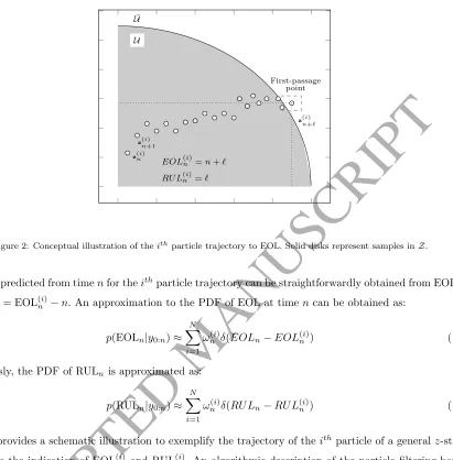
Figure 2: Conceptual illustration of theithparticle trajectory to EOL. Solid disks represent samples inZ.
The RUL predicted from timenfor theithparticle trajectory can be straightforwardly obtained from EOL(i)
n
as RUL(ni)= EOL(ni)−n. An approximation to the PDF of EOL at timencan be obtained as:
p(EOLn|y0:n)≈ N
X
i=1
ω(i)
n δ(EOLn−EOL(ni)) (14)
Analogously, the PDF of RULn is approximated as:
p(RULn|y0:n)≈ N
X
i=1
[image:10.595.95.506.110.528.2]ωn(i)δ(RU Ln−RU L(ni)) (15)
Figure 2 provides a schematic illustration to exemplify the trajectory of theithparticle of a generalz-state
along with the indication of EOL(ni) and RUL(ni). An algorithmic description of the particle filtering-based
prognostics procedure is provided as Algorithm 2.
3. Prognostics using Subset Simulation
3.1. Basis of Subset Simulation
Subset Simulation method is an efficient simulation framework originally proposed for computing small failure probabilities for general reliability problems [24]. It is motivated by the observation that the
simu-lation of a rare event can be transformed into the simusimu-lations of successive intermediate events with larger
probabilities. The small probability of the rare event can then be expressed as a product of larger conditional
probabilities that can be obtained with much less computational effort. In Subset Simulation, the conditional
ACCEPTED MANUSCRIPT
Algorithm 2Standard PF-prognostic algorithm
Inputs: nz(ni)=
x(ni), θ(ni)
, ωn(i)
oN
i=1 {updated particles at timen. Use Algorithm 1}, ¯U ⊂ Z {failure domain},
Outputs: EOLn, RU Ln
Begin (t>n):
1: fori= 1, . . . , N do
2: t←n
3: zt(i)←z
(i)
n
4: EvaluateEOL(ni)(z(ti)), {use Eq. 12 & 13}
5: whileI( ¯U)(z
(i)
t ) = 0do
6: Sampleθ(t+1i) ∼p(θt+1|θt(i))
7: Samplex(t+1i) ∼p(xt+1|x(ti), θ
(i)
t )
8: t←t+ 1
9: zt=x(ti), θ
(i)
t
←zt+1=
x(ti+1) , θ
(i)
t+1
10: end while
11: EOL(ni)←t, RU Ln(i)=EOL(ni)−n
12: end for
a performance functiong:Z →Rin a progressive manner. Let us assume that, with no loss of generality, ¯
U can be expressed through evaluation of exceedance of the performance function g above some specified threshold levelb, as follows:
¯
U ,{z∈ Z:g(z)> b} (16)
Let us also assume that the failure region ¯U is defined as the intersection of m nested regions in Z, i.e., ¯
U1 ⊃U¯2. . . ⊃U¯m−1 ⊃U¯m = ¯U, so that ¯U =Tmj=1U¯j. Each subset ¯Uj is typically termed as intermediate
failure domain and can be defined as1 ¯
Uj ,{z∈ Z :g(z)> bj}, withbj+1 > bj. Note that when ¯Uj holds,
then{U¯j−1, . . . ,U¯1} also hold, and henceP( ¯Uj|U¯j−1, . . . ,U¯1) =P( ¯Uj|U¯j−1), so it follows that2:
P( ¯U) =P m
\
j=1
¯
Uj
=P( ¯U1)
m
Y
j=2
P( ¯Uj|U¯j−1) (17)
whereP( ¯Uj|U¯j−1)≡P(z ∈U¯j|z∈U¯j−1), the conditional probability for the (j−1)th intermediate failure
domain, which is denoted byPj hereinafter for simplicity. Equation 17 indicates that the probability P( ¯U)
may be relatively small, however it can be approximated by Subset Simulation as the product of larger
conditional probabilities, thus avoiding simulation of rare events.
1It is assumed thatz
ndescribes a monotonically increasing process. In the contrary case, ¯Uj≡ {z∈ Z:g(z)< bj}, where
bj+1< bj.
ACCEPTED MANUSCRIPT
ACCEPTED MANUSCRIPT
3.2. Using Subset Simulation for prognosticsIn this section, Subset Simulation method is exploited as an efficient sampler for prognostics involving
rare-event simulation. As previously mentioned in Section 2, a prognostics algorithm aims at obtaining
sim-ulations of the model within the failure region whereby EOL/RUL estimations are subsequently derived. Let
p(zn:n+`|y0:n,U¯) ∝ p(zn:n+`|y0:n)IU¯(zn:n+`) denotes the PDF of `-step ahead predicted states distributed
within the region ¯U, so that p(zn:n+`|y0:n) represents the probability model for predictedz-states for the
interval (n:n+`], `> 1, which can be obtained by Total Probability theorem using the state transition
equationp(zt|zt−1) (see [2, 11] for further insights about predicting future states from the transition
equa-tion). The probability of expected performance of the predicted z-states within ¯U can be obtained as a
probability integral, i.e.,P( ¯U) =RU¯p(zn:n+`|y0:n)dzn:n+`, which can be approximated using Subset
Simula-tion as a product of condiSimula-tional probabilities as stated by EquaSimula-tion 17. The termP1 from Equation 17 can
be readily estimated by the standard Monte Carlo method (MC) as follows:
P( ¯U1)≈P¯1=
1
M M
X
k=1 IU¯1
zn1,:(nk+)` (18)
wherezn1,:(nk+)` Mk=1 areM samples simulated according to the PDFp(zn:n+`|y0:n). The superscript “1” here
indicates that such samples lie within the region ¯U1. The remaining factors can be efficiently estimated when
j>2 by conditional sampling fromp(zn:n+`|y0:n,U¯j−1)∝p(zn:n+`|y0:n)IU¯j
−1(zn:n+`), giving:
P( ¯Uj|U¯j−1)≈P¯j =
1
M M
X
k=1 IU¯j
znj−:n1+,(`k) (19)
where znj−:n1+,(`k) ∼ p(zn:n+`|y0:n,U¯j−1), and IU¯j(znj−:n1+,(`k)) is an indicator function for the region ¯Uj, j =
1, . . . , m, that assigns a value of 1 when g(zjn−:n1+,(`k)) > bj, and 0 otherwise. Note that, by virtue of the
Markov property of the state-space model,p(zn:n+`|y0:n) can be approximated by conditional sampling
us-ing recursively the one-step transition equation p(zn|zn−1) [2], i.e.: first samplezn(k+1) using the recurrence
given by the one-step transition equation conditional on the statezn, i.e.,zn(k+1) ∼p(·|zn); then sample the
succeeding state conditional on the previous sample, i.e.,z(nk+2) ∼p(·|z (k)
n+1); finally, repeat the same process
until the time indexn+`has been reached. Observe that in Subset Simulation for prognostics, there is no
need to invoke Markov chain Monte Carlo methods [38] for conditional sampling as was originally proposed
in [24], since conditional samples are straightforwardly obtained by simulating the state transition equation,
as has just been explained above.
Note also that it is possible to obtain samples that are generated at the (j−1)th level which lie in the
subsequent level ¯Uj. They are samples conditional on ¯Uj and provide “seeds” for simulating more samples
according to p(zn:n+`|y0:n,U¯j) [39]. Moreover, in Subset Simulation the choice of intermediate levels can
ACCEPTED MANUSCRIPT
n−1 n · · · n+`−1 n+`
M particles ¯ U U final threshold Z -space
Predicted particle trajectories Particles inZ-space
Measured data
n−1 n · · · n+`−1 n+` ¯ U ¯ Uj U Fix intermediate threshold intermediate threshold Z -space
n−1 n · · · n+`−1 n+` M P0samples
Selection of
M P0samples
¯ U ¯ Uj U Z -space 6
n−1 n · · · n+`−1 n+` ¯ U seed ¯ Uj U Generation of
M(P0−1) samples
Z
-space
n−1 n · · · n+`−1 n+` ¯
U
Msamples
Higher particle density around the threshold
Z
-space
Figure 3: Schematic representation of conditional samples produced using PFP-SubSim algorithm.
among the valuesg(znj−:n1+,(`k)), so that the sample estimate ofP( ¯Uj|U¯j−1) in Equation 19 is equal to a fixed
valueP0 ∈ (0,1). Therefore, ¯Uj is adaptively chosen based on the samples znj−:n1+,(`k) M
k=1 generated from
p(zn:n+`|y0:n,U¯j−1), in such a way that there are exactly M P0of these samples in ¯Uj, which serve as seeds
for generating more samples according top(zn:n+`|y0:n,U¯j) [39, 40]. In fact, the remaining (1/P0−1) samples
are generated fromp(zn:n+`|y0:n,U¯j) by simulating the state space model starting at each seed, giving a total
ofM samples in ¯Uj. This procedure is repeated for higher conditional levels until the final region ¯Um= ¯U
has been reached. The PDF of EOL/RUL can be straightforwardly obtained by applying Equations 12 to 15
using as samples those distributed within the final region ¯Um. A schematic representation of the main steps
of the proposed Subset Simulation approach has been provided in Figure 3. These steps can be summarized
as follows (the sequence is indicated by the arrows in Figure 3): (i) generation of`-step ahead predictive
samples from p(zn|y0:n); (ii) adaptive fixing of the intermediate threshold value bj; (iii) definition of the
intermediate region ¯Uj so that P( ¯Uj|U¯j−1) = P0; (iv) generation of new samples distributed according to
p(·|y0:n,U¯j), j= 1, . . . , m, (v) calculation of EOL/RUL using theM samples from the final subset.
3.3. The PFP-SubSim algorithm
ACCEPTED MANUSCRIPT
ACCEPTED MANUSCRIPT
that a fixed amount ofM samples are drawn per simulation level ¯Uj, so thatNT =mM, the total amount
of model evaluations required by the algorithm to reach the final threshold. It is important to remark that
this choice is just to allow the computational cost to be controlled.
Algorithm 3Pseudocode implementation for PFP-SubSim
Inputs: P0 ∈(0,1){gives percentile selection, chosen soN P0,1/P0∈Z+;P0 = 0.2 is recommended}, M {number
of samples per simulation level},b∈R{threshold value},nzn(i)=
x(ni), θ(ni)
, ω(ni) oN
i=1{e.g. use Algorithm 1}
Outputs: EOLn, RU Ln
Begin:
1: Samplezn(1), . . . , z(nN)
, according to weightsωn(i) Ni=1
2: Setk= 0,j= 0
3: fori: 1, . . . , N do
4: t←n
5: zt(i)←z
(i)
n
6: repeat
7: Samplez(t+1i) ∼p(zt+1|zt(i))
8: t←t+ 1
9: k←k+ 1
10: zt(i)←zt(i+1)
11: zj,(k)←zt(i)
12: Evaluateg(jk)=g zj,(k)
13: untilt=n+`, `=M/N
14: end for
15: Sortzj,(k) M
k=1so thatg (1)
j 6g
(2)
j 6. . .6g
(M)
j {g
(1)
j >g
(2)
j >. . .>g
(M)
j for decreasing processes}
16: bj←1 2
g(M P0)
j +g
(M P0+1) j
17: whilebj< b {Setbj> bfor decreasing processes} do
18: j←j+ 1
19: fork= 1, . . . , M P0 do
20: Select as a seed zj,(k),(1)= zj−1,(k)∼p z|U¯j
21: Sample from Eq. (5) to generate 1/P0 states of a Markov chain lying in ¯Uj:
zj,(k),(1), . . . , zj,(k),(1/P0)
22: end for
23: Renumbernzj,(k),(i)oM P0,1/P0 k=1,i=1 as
zj,(1), . . . , zj,(M)
24: Sortzj,(k) M
k=1so thatg (1)
j 6g
(2)
j 6. . .6g
(M)
j {g
(1)
j >g
(2)
j >. . .>g
(M)
j for decreasing processes}
25: bj←1 2
g(M P0)
j +g
(M P0+1) j
26: end while
27: m←j
28: EvaluateEOL(nk) M k=1,
RU L(nk)=EOL(nk)−n M
ACCEPTED MANUSCRIPT
In the proposed algorithm, the choice of a suitableP0value has a significant impact, since a small value
(P0→0) makes the distance between consecutive intermediate levelsbj−bj−1 to become too large, which
leads to a rare-event simulation problem [39, 41]. If, on the contrary, the intermediate threshold values
were chosen too close (P0 → 1), the algorithm would require a large total number of simulation levels m
(and hence high computational effort) to reach the target region ¯U. A rational choice forP0 should strike a
balance between both extreme cases. In the original presentation of Subset Simulation in [24],P0= 0.1 was
recommended, and in [39], the range 0.16P060.3 was found to be near optimal after a rigorous sensitivity
study of Subset Simulation. More recently, in [40] the valueP0 = 0.2 was found to be optimal for Subset
Simulation in application to Approximate Bayesian Computation problems. Following the recommendation
by [39, 40], the conditional probabilityP0 is conveniently chosen here so that M P0 and 1/P0 are positive
integers, thusP0is set to 0.2.
In Algorithm 3, the time subscripts are dropped from step 12 for simplicity, since the time indexing is
prescribed in each sample. Observe that the proposed methodology, and in particular the steps 20 and 21
in Algorithm 3, have anticipated that the multi-step ahead predicted trajectories simulated according to
the model (Equation 2) can be split into seeds whereby subsequent states are generated, without artificially
influencing the recurrence given by the stochastic process. This is justified by the Markovian assumption,
so that the probability of obtainingzn+` depends only on its preceding statezn+`−1 and not on the history
of past states. The last implies that the simulation of a sequence of states`−step ahead is essentially an
uncoupled procedure given the information from the previous step.
4. Illustrative examples
4.1. Toy example
Consider an exponential degradation process described by the following discrete state-transition equation:
xn =e−2ζnxn−1+vn (20)
wherexn ∈Rare discrete system states for n∈N, ζ ∈Ris the decay parameter, a scaling constant that
controls the degradation velocity, andvn∈Ris the model error term which is assumed to be modeled as a
zero-mean Gaussian distribution, i.e.vn ∼ N(0, σv). Let us now assume that the degradation process can be
measured over time and that, at a certain timen, the measured degradation can be expressed as a function
of the latent damage statexn, as follows:
yn=xn+wn (21)
ACCEPTED MANUSCRIPT
ACCEPTED MANUSCRIPT
n
0 20 40 60 80 100 120
yn
-0.5 0 0.5 1
Data
Filtered estimate (mean) 5-95% probability band
(a)
n
0 20 40 60 80 100 120
yn
-0.5 0 0.5 1
b1=0.54475
Data
Filtered estimate (mean) 5-95% probability band
(b)
n
0 20 40 60 80 100 120
yn
-0.5 0 0.5 1
b1=0.54475 b2=0.41087 b
Data
Filtered estimate (mean) 5-95% probability band
(c)
EOLn
0 20 40 60 80 100 120
0 0.02 0.04 0.06
[image:16.595.59.509.109.442.2](d)
Figure 4: PFP-SubSim output for the exponential degradation model in Eq. 20 by usingζ = 0.015. Predicted samples are
represented in the state-space forn+`, n= 10, `>1 using circles.
are selected as model parameters, i.e. θ = (σv, σw) ∈ R2. The uniform PDF U(0.0001,0.2) is used as
component-wise prior information about the model parametersθ1=σvandθ2=σw. Degradation states are
initialized atx0= 0.9, expressed in arbitrary units. Synthetic data foryn is used by generating them from
Equations 20 and 21 consideringθtrue = (0.01,0.02). The PFP-SubSim results predicted at time n = 10
are presented in Figure 4 for three different simulation levels (m= 3) by using P0 = 0.2. A total amount
of N = 1000 particles trajectories are employed by Algorithm 1 (in this example, the resampling step is
run every time new data are collected). A zero-mean Gaussian has been used for the artificial evolution of
model parameters, i.e.p(θn|θn−1)∼ N(0, Wn), whereWn= 5·10−4I2, beingI2the identity matrix of order
2. Finally, the failure region is defined by fixing a threshold value for the states of 0.3, expressed in arbitrary
units, i.e. ¯U ={xn∈R:xn <0.3}.
In panel 4a, predicted samples are represented in the state-space forn+`, n= 10, `>1 using circles. In panels
4b and 4c, samples are increasingly distributed in subsets according top(zn:n+`|y0:n,U¯j), j = 1,2. They
ACCEPTED MANUSCRIPT
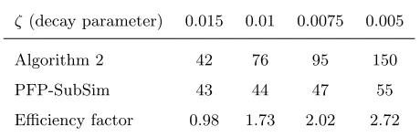
ζ (decay parameter) 0.015 0.01 0.0075 0.005
Algorithm 2 42 76 95 150
PFP-SubSim 43 44 47 55
[image:17.595.171.401.106.181.2]Efficiency factor 0.98 1.73 2.02 2.72
Table 1: Results of the comparative exercise between PFP-SubSim and Algorithm 2 for the exponential decay model of Eq. 20.
4d shows the histogram representation of the PDFp(EOLn|y0:n) predicted at timen = 10. The triangle
represents the time when the threshold valueb= 0.3 is reached according to the synthetic data. Observe that
by using PFP-SubSim algorithm, the`-step ahead predicted samples are distributed in subsets which are
increasingly closer to the final threshold. The final subset (represented using dark purple circles in Figure 4c) encloses a considerable amount of samples distributed around the vicinity of the threshold, hence increasing
the resolution of the PDF of EOL without the need of employing big amounts of model evaluations that
unnecessarily increases the computational cost.
A comparative study has been carried-out to reveal the computational efficiency that can be gained using
PFP-SubSim against Algorithm 2 for obtaining the PDF of EOL. For this exercise, the amount of model
evaluations needed to produce one sample simulated according to the PDFp(EOLn|y0:n) is monitored at
n= 10. In other words, the focus is on the ratio defined by the amount of samples that describep(EOLn|y0:n)
over the total amount of model evaluations employed by each of the algorithms used for comparison. The
results, shown in the second and third rows of Table 1, are obtained by considering different values for the
decay parameterζin Equation 20. The values shown were obtained considering the mean of 200 independent
runs of the algorithms, a large enough number of runs to ensure the convergence of the values represented in Table 1. The efficiency factor (forth row) is obtained by division operation of the values from the third row
by those from the second row, and is indicative of the computation time that can be saved by PFP-SubSim
algorithm as compared to Algorithm 2. Observe that the results are fairly similar whenζ is high because
reaching the final threshold is not in this case a rare event under the model given by Equation 20. However,
lower values of the decay parameterζimplies that reaching the threshold is less probable or even a rare event
under the model, which is precisely the situation when PFP-SubSim exploits its higher efficiency. Indeed,
note from Table 1 that about2/3of the model evaluations can be saved by using PFP-SubSim algorithm as
compared to Algorithm 2 for the lowest value ofζ, i.e.ζ= 5×10⁻³(fifth column), which implies an efficiency
factor of 2,72. These results about PFP-SubSim efficiency will be further corroborated in the context of the
ACCEPTED MANUSCRIPT
ACCEPTED MANUSCRIPT
4.2. Case study: Prediction of fatigue damage using monitoring dataIn this section, the performance of the algorithm is investigated through a case study about damage
prognostics in carbon fibre reinforced polymer (CFRP) laminates using structural health monitoring (SHM)
data. In previous works by the authors [2, 11], a model-based prognostics methodology was presented
which demonstrated efficiency for long-term predictions of fatigue damage in cross-ply laminates using SHM data. To avoid duplication of literature for this technique but conferring a sufficient conceptual framework,
the relevant details from the referred methodology are presented here in a concise manner.
The starting point of this methodology involves the calculation ofG, the energy released per unit crack
area due to the formation of a new crack between two existing cracks as [42, 43]:
G= σ
2
xh
2ρt90
1
E∗
x(2ρ)−
1
E∗
x(ρ)
(22)
where σx is the maximum applied axial tension, and h and t90 are the laminate and 90◦-sublaminate
half-thickness, respectively. The matrix micro-cracks density is denoted byρ= 1
2¯l, where ¯l is the half
crack-spacing normalized by the 90◦ sub-laminate thickness. The term E∗
x(ρ), as a function of ρ, is the effective
Young’s modulus due to the current damage state which can be modeled through micro-damage mechanics
models [44]. In this case study, the shear-lag [45, 46] micro-damage model is adopted to be simpler and
robust [47], such that:
Ex∗=
Ex,0
1 +a2¯1lR(¯l) (23) whereEx,0is the undamaged longitudinal Young’s modulus of the overall laminate, andais a function of the
mechanical and geometrical properties of the laminate, which can be obtained using the classical laminate
plate theory [48] (see also [49] for further details about the calculation ofa). The termR(¯l), known as the
average stress perturbation function, is defined by [47]:
R(¯l) =2
ξtanh(ξ¯l) (24)
where
ξ2=Gyz
1
Ey
+ t90
tφEx(φ)
!
(25)
In the last equation,Gyz, Ey, andEx(φ)are laminate mechanical parameters which are described next. The
details about the geometry parameters involved in Equations 22 to 25, together with information about the
pattern of micro-cracks, are given in Figure 5.
Next, the modified Paris’ law [50] is used to model the evolution of matrix micro-cracks density as a function of fatigue cyclen∈N, as follows:
ρn=ρn−1+A(∆G(ρn−1))α (26)
whereAandαare fitting parameters. The term ∆Gis the increment of energy release (recall Equation 22)
ACCEPTED MANUSCRIPT
Figure 5: Illustration for microscopic damage pattern in
φnφ
2
/90n90/φnφ 2
laminate along with basic geometrical parameters.
4.2.1. Stochastic embedding
The progression of damage is modeled at every cyclenby focusing on the matrix-cracks densityρn and
the normalized effective stiffnessDn=Ex∗/Ex,0, defining a joint state transition equation of two components
as follows:
x1n=ρn=f1n(ρn−1, θ)
| {z }
Eq. (26)
+v1n (27a)
x2n=Dn=f2n(ρn, θ)
| {z }
Eq. (23)
+v2n (27b)
wherexn= (x1n, x2n)∈R
2 is the actual system response at timen. Subscripts 1 and 2 correspond to the
damage subsystems, namely, matrix-crack density and normalized effective stiffness, respectively. The vector
vn = (v1n, v2n)∈ R
2 corresponds to the model error vector of the overall system, which, by the Principle
of Maximum Information Entropy (PMIE) [51–53], is chosen as a Gaussian, i.e.vn ∼ N 0,σv1n, σv2n
I2,
whereσv1n, σv2n
are the standard deviations ofvn andI2 is the identity matrix of order 2, so they can be
readily sampled.
Let us now consider that the vector yn = y1n, y2n
= ˆρn,Dˆn represents the measurements of the
system outputxn and also that a measurement function is added to the state-space model to account for
the measurement errorwn∈R2:
y1n= ˆρn=x1n+w1n (28a)
y2n= ˆDn =x2n+w2n (28b)
where ˆρn,Dˆn denote the measured matrix-cracks density and normalized effective stiffness, respectively. As
stated before, the PMIE is used to choose wn to be distributed as zero mean Gaussian PDF, i.e. wn ∼
ACCEPTED MANUSCRIPT
ACCEPTED MANUSCRIPT
and geometrical parameters describing Equations 22 to 26 (see Table 2) through a Global Sensitivity Analysis
based on variances [49, 54], resultingθ= α, Ex, Ey, t, σv1n, σv2n
as the vector of model parameters. The
rest of parameters can be fixed at some point within their range of variation, (e.g. the mean value) without
significantly influencing the output uncertainty.
4.2.2. Results
For the prediction of the PDF of EOL/RUL, SHM measurements of micro-cracks density and stiffness
reduction from a fatigue test are considered for a 15.24×25.4 [cm] laminate coupon with dogbone geometry
and [02/904]s stacking sequence. The mechanical properties along with their probabilistic information are
listed in Table 2. In this example,a= 0.1325 (recall Equation 23), according to [49]. The test was conducted
under load-controlled tension-tension fatigue loadings with a frequency off = 5 [Hz], and maximum applied
loads of 31.13 [KN], which represents an equivalent maximum stress of 80% of their ultimate stress. The
ratio between the minimum and maximum applied stress per cycle was set to 0.14. Further details about
this test can be found in [55] and also in the Composites dataset, NASA Ames Prognostics Data Repository
[56] (damage data used in this example correspond to laminate L1S19). In [57], the details about the SHM
methodology are provided. A summary of the dataset used for this study is extracted from [56] and provided here in Table 3.
At each prognostic step, which corresponds to each of the fatigue cycles when SHM data are available
as shown in the first row of Table 3, Algorithm 1 is run by using N = 5000 particles and systematic
importance resampling. Initial values for the damage states arex0 = (ρ0, D0), where ρ0 = 0.1 [cracks/mm]
andD0= 1 (dimensionless). The standard deviation of the measurement error parameters are set toσw1,n=
0.05 [cracks/mm] and σ
w2,n = 0.01, taking them as known. Chosen prior PDFs for model parameters θ =
(θ1, θ2, . . . θ6) are specified in Table 2. The diagonal elements of the covariance matrixWn(recall Equation 6)
are appropriately selected through initial test runs and set to 0.5% of the 5th-95th band of the prior PDFs
for thejthcomponent of θ.
Updated damage states at time n are propagated forward in time by using PFP-SubSim algorithm. For illustration purposes, results of micro-cracks density and stiffness loss are shown in Figure 6 for prediction
time n = 3 ·104. Three simulation levels (m = 3) are employed in Figure 6 by using P
0 = 0.5 and
M = 2.4·104samples per simulation level. The total amount of samples is thusN
T = (2.4 + 1.2 + 1.2)·104,
becauseM P0= 1.2·104 samples from each conditional level are used as seeds to start the next simulation
level. In Figure 6, the triangles represent the time (in cycles) when matrix micro-cracks density will reach
the final thresholdb= 418 [#cracks·m−1], together with its associated threshold for stiffness 0.88, which
are known from [56], and also shown in Table 3. These thresholds define a failure region given by ¯U =
{(ρn, Dn)∈R2: 0< ρn<418,0< Dn <0.88}.
ACCEPTED MANUSCRIPT
different subsets, since the recommended near-optimal value ofP0 = 0.2 for Subset Simulation produced
m= 1 conditional levels for the majority of times of prediction. The estimation of RUL by PFP-SubSim
algorithm is plotted against time in Figure 7. The results shown in Figure 7 are satisfactory in the sense
Type Parameter Nominal value Units Prior PDF
Mechanical Ex 127.55·109 Pa LN(ln(127.55·109),0.1)
Ey 8.41·109 Pa LN(ln(8.41·109),0.1)
Gxy 6.20·109 Pa Not applicable
Gyz 2.82·109 Pa Not applicable
νxy 0.31 – Not applicable
Geometrical t 1.5·10−4 m
LN(ln(1.5·10−4),0.1)
Fitting α 1.80 – LN(ln(1.80),0.2)
A 1·10−4 – Not applicable
Errors σv1 –
# cracks
m·cycle U(0.5,1.5)
σv2 – – U(0.001,0.003)
Table 2: Prior information and nominal values of main parameters used in calculations.
Fatigue cycles 101 102 103 104 2·104 3·104 4·104 5·104 6·104 7·104 8·104 9·104
ρ[# cracks/m] 98 111 117 208 270 305 355 396 402 402 407 418
[image:21.595.131.486.175.363.2]D 0.954 0.939 0.930 0.924 0.902 0.899 0.888 0.881 0.896 0.872 0.877 0.885
Table 3: Experimental sequence of damage for cross-ply [02/904]s CFRP laminate. The data are presented for micro-cracks
density (ρ) and normalized effective stiffness (D).
n(cycles)
×104
0 2 4 6 8 10
ρ
n
0 200 400 600 800
b= 418
(a)
n(cycles)
×104
0 2 4 6 8 10
D
n
0.75 0.8 0.85 0.9 0.95 1
0.88
(b)
Figure 6: PFP-SubSim output for predicting (a) matrix micro-cracks density and (b) normalized effective stiffness atn=
[image:21.595.70.507.396.665.2]ACCEPTED MANUSCRIPT
ACCEPTED MANUSCRIPT
0 1 2 3 4 5 6 7 8 9x 10⁴ 0
1 2 3 4 5 6 7 8 9x 10
4
n
R
U
L
n
[(1−0.2)RUL*,(1+0.2)RUL*] [(1−0.1)RUL*,(1+0.1)RUL*] RUL*
estimated RUL
Figure 7: Results for RUL predictions together with their quantified uncertainty by the interquartile bars.
that the proposed algorithm has the ability to obtain the RUL with high precision, except in the first stage
of the fatigue process, which corresponds to the interval of cycles required for the data to train the model
parametersθ. To help evaluating the prediction accuracy and precision, two shaded cones of accuracy are used
at 10% and 20% of the true RUL, denoted here as RUL∗, following the methodology given by [58]. Observe also from Figure 7 that accuracy seems to depart from true RUL at the final stage, in the sense that the
estimated mean values for the RUL (labeled by the gray circles) leave progressively the accuracy area as
fatigue cycles evolve fromn= 5·104. Such behavior has been previously reported in [2, 11] and was found to be related with the asymptotic behavior of the damage progression in composites.
4.2.3. Discussion
In this section, comparative exercises have been carried out to investigate the computational improvement
and accuracy that can be achieved using PFP-SubSim algorithm with respect to a traditional prognostics
algorithm, like Algorithm 2. It should be noted that the results shown here are extensible to other applications different than composite materials, since they are focused on efficiency aspects about the simulation engines
of the competing algorithms.
The first exercise of interest regards the evaluation of the probability of prospective failure during a
prescribed interval of future instants (n, n+`]⊂N, as follows:
P( ¯U) =
Z
¯
U
p(zn:n+`|y0:n)dzn:n+`≈ 1 NT
NT X
k=1
ACCEPTED MANUSCRIPT
0 2 4 6 8 10
x 104 0.2
0.4 0.6 0.8 1
cycles
P
(
¯U)
Algorithm 2 PFP−SUBSIM
(a)
cycles ×104
0 2 4 6 8 10
C
P
U
ti
m
e
[s
ec
]
10-1 100 101 102 103
(b)
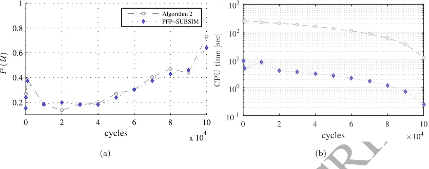
Figure 8: (a) Plots forP( ¯U) estimation using PFP-SubSim algorithm in comparison to Algorithm 2 used as benchmark. (b)
CPU time employed by each algorithm, represented in logarithmic scale and expressed in seconds.
where zn(k:n)+` NT
k=1 are NT predictive samples simulated according to the PDF p(zn:n+`|y0:n). Note that
the approximation given by Equation 29 is equivalent to the standard Monte Carlo method for evaluating
probability integrals as a mathematical expectation. Note also that this method has a well-known drawback
in cases of small values for P( ¯U), by the fact that a huge number of simulations are required to achieve acceptable estimation accuracy, which may increase the computational cost significantly. By PFP-SubSim,
P( ¯U) can be straightforwardly evaluated via the the conditional probabilities involved in Subset Simulation
(recall Equation 17):
P( ¯U) =P( ¯U1)
m
Y
j=2
P( ¯Uj|U¯j−1)≈P0m (30)
Figure 8a shows estimations of the probability of prospective failureP( ¯U) obtained at different prediction
instantsnusing comparatively the simulation engines of PFP-SubSim algorithm and Algorithm 2. To avoid
an excessive computational cost for this exercise, the simulations are restricted to lie within the interval
(n,105]⊂N, since such interval is enough to highlight the differences between both algorithms. The CPU
times required by each algorithm are plotted against the prediction instants in Figure 8b, which have been
obtained using a 3.5 GHz double-core system. The results shown for Algorithm 2 were obtained using a large enough amount of samples for the estimation ofP( ¯U) to be sufficiently accurate, hence used here as
benchmark values. Observe that the estimations of P( ¯U) produced by PFP-SubSim algorithm agree well
with the benchmark values given by Algorithm 2, even when PFP-SubSim requires significantly less CPU
time. Note also that the predicted probability values are high in comparison toP0= 0.2, hence a significant
improvement in efficiency is expected for PFP-SubSim algorithm if the comparison is performed for failure
[image:23.595.79.497.116.281.2]ACCEPTED MANUSCRIPT
ACCEPTED MANUSCRIPT
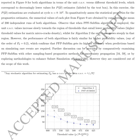
since it gives a measure of efficiency that is inherent to the algorithm because it is invariant to the number of
simulated samples3[25]. This is of special interest for our exercise since the total amount of samples required
by PFP-SubSim algorithm varies depending on the failure probability value to be estimated. The results are
reported in Figure 9 for both algorithms in terms of the unit c.o.v. versus different threshold levels, which
correspond to decreasingly lower values forP( ¯U) estimates (labeled by the text box). In this exercise, the
P( ¯U) estimations are evaluated at cyclen= 8·104. To quantitatively assess the statistical properties for the
prognostics estimates, the numerical values of each plot from Figure 9 are obtained by considering the mean
of 200 independent runs of both algorithms. Observe that when PPF-SubSim algorithm is employed, the
unit c.o.v. values increase slowly towards the region of thresholds that entail lower probability values (higher
threshold values for matrix micro-cracks density), whilst for Algorithm 2 the unit c.o.v. grows steeply in that region. However, the performance of both algorithms is fairly similar for higher probability values, (say of
the order ofP0 = 0.2), which confirms that PFP-SubSim gets its highest efficiency when predictions based
on simulating rare events are required. Further discussion can be provided by comparatively examining
PFP-SubSim with other sampling-based prognostics methods for uncertainty propagation [34, 59], or by
exploring methodologies to enhance Subset Simulation efficiency [60]. However they are considered out of
the scope of this work.
3Any stochastic algorithm for estimatingP¯
U has a c.o.v. of the form c.o.v. =4/pNT
600 575 550 525 500 475 450 425
50 100 150 200 250 300 350
0.012
0.022
0.047
0.098 0.16
0.24 0.33
0.4
Threshold value ρ[#cracks
m ]
Unit
co
v
(
4
)
[image:24.595.48.521.157.648.2]Algorithm 2 PFP-SUBSIM
Figure 9: Results for the unit c.o.v. ofP( ¯U) obtained using PFP-SubSim algorithm as compared to that obtained using
ACCEPTED MANUSCRIPT
5. Conclusions
This paper presented a novel prognostics algorithm, the PFP-SubSim algorithm, that combines the
prog-nostics principles with the Subset Simulation method. The algorithm gets its efficiency by adaptively drawing
samples over a nested sequence of intermediate failure regions (subsets), until a predefined final region is reached. These regions were defined in an adaptive manner, which avoids preliminary calibrations. An
exam-ple of application along with a case study were provided to illustrate the computational efficiency that can
be gained with PFP-SubSim. The results indicated that our algorithm is highly efficient for the prognostics
of processes involving rare-event simulations, whilst its behavior is fairly similar to a standard prognostics
algorithm when probabilities are not so small. For that reason, PFP-SubSim can be considered as a general
purpose prognostics algorithm, which is specially suited for rare-event prediction. Further research is needed
to investigate the extension of the proposed algorithmic framework for the case of multidimensional state
spaces (saynz >10). In particular, an improvement of much interest would be the application of adaptive
methods to optimally scale the artificial evolution of the model parameters in multidimensional state spaces.
Acknowledgment
Dr. Manuel Chiach´ıo is a Research Fellow of the Lloyd’s Register Foundation (LRF), a charitable
foun-dation in the UK helping to protect the life and property by supporting engineering-related education,
public engagement, and the application of research. The two first authors would like to specially thank the
Prognostics Center of Excellence at NASA Ames, which kindly hosted them during part the course of this
work. Authors would also like to thank the Structures and Composites Lab (under auspices of Prof. Fu-Kuo Chang) at Stanford University for experimental data, and NASA ARMD/AvSafe project SSAT, which
provided partial support for this work. Finally, they would also like to thank Prof. James L. Beck from
California Institute of Technology and Dr. Abhinav Saxena from General Electric Global Research, for their
ACCEPTED MANUSCRIPT
ACCEPTED MANUSCRIPT
References
[1] J. Chiach´ıo, M. Chiach´ıo, A. Saxena, K. Goebel, Prognostics design for structural health management, in: Emerging
Design Solutions in Structural Health Monitoring Systems, IGI Global, 2015, pp. 234–273.
[2] M. Chiach´ıo, J. Chiach´ıo, A. Saxena, K. Goebel, An energy-based prognostic framework to predict evolution of damage
in composite materials, in: Structural Health Monitoring (SHM) in Aerospace Structures, Woodhead Publishing-Elsevier,
2016, pp. 447–477.
[3] R. Reinertsen, Residual life of technical systems; diagnosis, prediction and life extension, Reliability Engineering and
System Safety 54 (1) (1996) 23–34.
[4] K. Javed, R. Gouriveau, N. Zerhouni, State of the art and taxonomy of prognostics approaches, trends of prognostics
applications and open issues towards maturity at different technology readiness levels, Mechanical Systems and Signal
Processing 94 (2017) 214–236.
[5] E. Zio, Reliability engineering: Old problems and new challenges, Reliability Engineering and System Safety 94 (1) (2009)
125–141.
[6] J. D. Andrews, T. R. Moss, Reliability and risk assessment, Professional Engineering Publishing Limited, 2002.
[7] D. An, N. H. Kim, J.-H. Choi, Practical options for selecting data-driven or physics-based prognostics algorithms with
reviews, Reliability Engineering & System Safety 133 (2015) 223–236.
[8] S. Sankararaman, K. Goebel, Uncertainty in prognostics and systems health management, International Journal of
Prog-nostics and Health Management 6 (010).
[9] P. Baraldi, F. Mangili, E. Zio, Investigation of uncertainty treatment capability of model-based and data-driven prognostic
methods using simulated data, Reliability Engineering & System Safety 112 (2013) 94–108.
[10] F. Cadini, E. Zio, Model-based Monte Carlo state estimation for condition-based component replacement, Reliability
Engineering and System Safety 94 (1) (2009) 752–758.
[11] J. Chiach´ıo, M. Chiach´ıo, S. Shankararaman, A. Saxena, K. Goebel, Condition-based prediction of time-dependent
relia-bility in composites, Reliarelia-bility Engineering and System Safety 142 (2015) 134–147.
[12] B. Saha, J. R. Celaya, P. F. Wysocki, K. F. Goebel, Towards prognostics for electronics components, in: Aerospace
conference, 2009 IEEE, IEEE, 2009, pp. 1–7.
[13] M. Daigle, S. Kulkarni, Electrochemistry-based battery modeling for prognostics, in: Proceedings of the Annual Conference
of the Prognostics and Health Management Society, 2013, Vol. 1, 2013, pp. 249–261.
[14] M. Jouin, R. Gouriveau, D. Hissel, M.-C. P´era, N. Zerhouni, Degradations analysis and aging modeling for health
assess-ment and prognostics of pemfc, Reliability Engineering & System Safety 148 (2016) 78–95.
[15] B. Saha, K. Goebel, J. Christophersen, Comparison of prognostic algorithms for estimating remaining useful life of
batteries, Transactions of the Institute of Measurement and Control 31 (3-4) (2009) 293–308.
[16] M. S. Arulampalam, S. Maskell, N. Gordon, T. Clapp, A tutorial on particle filters for online nonlinear/non-Gaussian
Bayesian tracking, Signal Processing, IEEE Transactions on 50 (2) (2002) 174–188.
[17] A. Doucet, N. De Freitas, N. Gordon, An introduction to sequentialMonteCarlo methods, in: A. Doucet, N. De Freitas,
N. Gordon (Eds.), Sequential Monte Carlo methods in practice, Springer, 2001, pp. 3–14.
[18] E. Zio, G. Peloni, Particle filtering prognostic estimation of the remaining useful life of nonlinear components, Reliability
Engineering and System Safety 96 (3) (2011) 403–409.
[19] M. Orchard, G. Kacprzynski, K. Goebel, B. Saha, G. Vachtsevanos, Advances in uncertainty representation and
manage-ment for particle filtering applied to prognostics, in: International Conference on Prognostics and Health Managemanage-ment
(PHM, 2008),IEEE, 2008, pp. 1–6.
[20] M. Daigle, K. Goebel, Multiple damage progression paths in model-based prognostics, in: Aerospace Conference, 2011
ACCEPTED MANUSCRIPT
[21] M. Daigle, K. Goebel, Model-based prognostics with fixed-lag particle filters, in: Proceedings of the Annual Conference
of the Prognostics and Health Management Society, 2009, Vol. 1, 2009, pp. 249–261.
[22] J. R. Celaya, A. Saxena, K. Goebel, Uncertainty representation and interpretation in model-based prognostics algorithms
based onkalman filter estimation, in: Annual Conference of Prognostics and Health Management Society, PHM Society,
2012, pp. 12–24.
[23] M. Corbetta, S. Sbarufatti, M. Giglio, Optimal tuning of particle filtering random noise for monotonic degradation
processes, in: Proceedings of the third European Conference of the Prognostics and Health Management Society, IEEE,
2016, pp. 479–489.
[24] S. Au, J. Beck, Estimation of small failure probabilities in high dimensions bySubsetSimulation, Probabilistic Engineering
Mechanics 16 (4) (2001) 263–277.
[25] S. Au, J. Ching, J. Beck, Application ofSubsetSimulation methods to reliability benchmark problems, Structural Safety
29 (3) (2007) 183–193.
[26] J. Ching, S. Au, J. Beck, Reliability estimation of dynamical systems subject to stochastic excitation using Subset
Simulation with splitting, Computer Methods in Applied Mechanics and Engineering 194 (12-16) (2005) 1557–1579.
[27] M. Chiach´ıo, J. Chiach´ıo, A. Saxena, K. Goebel, An efficient simulation framework for prognostics of asymptotic
processes-a cprocesses-ase study in composite mprocesses-ateriprocesses-als., in: Proceedings of the Europeprocesses-an Conference of the Prognostics processes-and Heprocesses-alth Mprocesses-anprocesses-age-
Manage-ment Society, Nantes, France 2014, PHM Society, 2014, pp. 202–214.
[28] E. My¨otyri, U. Pulkkinen, K. Simola, Application of stochastic filtering for lifetime prediction, Reliability Engineering
and System Safety 91 (2) (2006) 200–208.
[29] N. Gordon, D. Salmond, A. Smith, Novel approach to nonlinear/non-Gaussian Bayesian state estimation,
IEEE-Proceedings-F 140 (1993) 107–113.
[30] J. Liu, M. West, Combined parameter and state estimation in simulation-based filtering, in: A. Doucet, N. Freitas,
N. Gordon (Eds.), Sequential Monte Carlo Methods in Practice, Statistics for Engineering and Information Science,
Springer New York, 2001, pp. 197–223.
[31] M. J. Daigle, K. Goebel, Model-based prognostics with concurrent damage progression processes, Systems, Man, and
Cybernetics: Systems, IEEE Transactions on 43 (3) (2013) 535–546.
[32] A. Doucet, S. Godsill, C. Andrieu, On sequentialMonteCarlo sampling methods forBayesian filtering, Statistics and
computing 10 (3) (2000) 197–208.
[33] J. Handschin, D. Q. Mayne, MonteCarlo techniques to estimate the conditional expectation in multi-stage non-linear
filtering, International Journal of Control 9 (5) (1969) 547–559.
[34] M. Jouin, R. Gouriveau, D. Hissel, M.-C. P´era, N. Zerhouni, Particle filter-based prognostics: Review, discussion and
perspectives, Mechanical Systems and Signal Processing 72 (2016) 2–31.
[35] J. Ching, J. L. Beck, K. A. Porter, R. Shaikhutdinov, Bayesian state estimation method for nonlinear systems and its
application to recorded seismic response, Journal of Engineering Mechanics 132 (4) (2006) 396–410.
[36] G. Kitagawa, MonteCarlo filter and smoother for non-Gaussian nonlinear state space models, Journal of computational
and graphical statistics 5 (1) (1996) 1–25.
[37] A. Kong, J. S. Liu, W. H. Wong, Sequential imputations andBayesian missing data problems, Journal of the American
statistical association 89 (425) (1994) 278–288.
[38] F. Liang, C. Liu, J. Chuanhai, AdvancedMarkov chainMonteCarlo methods, Wiley Online Library, 2010.
[39] K. Zuev, J. Beck, S. Au, L. Katafygiotis, Bayesian post-processor and other enhancements of Subset Simulation for
estimating failure probabilities in high dimensions, Computers & Structures 93 (2011) 283–296.


![Table 3: Experimental sequence of damage for cross-ply [0ACCEPTED MANUSCRIPT2/904]s CFRP laminate](https://thumb-us.123doks.com/thumbv2/123dok_us/8567572.367510/21.595.70.507.396.665/table-experimental-sequence-damage-cross-accepted-manuscript-laminate.webp)