An Improvement of Pedestrian Detection Method with Multiple Resolutions

ISSN Online: 2327-5227 ISSN Print: 2327-5219

An Improvement of Pedestrian Detection

Method with Multiple Resolutions

Guodong Zhang

1

, Peilin Jiang

2

, Kazuyuki Matsumoto

1

, Minoru Yoshida

1

, Kenji Kita

1

1_{Faculy and School of Engineering, Tokushima University, Tokushima, Japan} 2_{Xi’an Jiaotong University, Xian, China}

Abstract

In object detection, detecting an object with 100 pixels is substantially differ-ent from detecting an object with 10 pixels. Many object detection algorithms assume that the pedestrian scale is fixed during detection, such as the DPM detector. However, detectors often give rise to different detection effects un-der the circumstance of different scales. If a detector is used to perform pede-strian detection in different scales, the accuracy of pedepede-strian detection could be improved. A multi-resolution DPM pedestrian detection algorithm is pro-posed in this paper. During the stage of model training, a resolution factor is added to a set of hidden variables of a latent SVM model. Then, in the stage of detection, a standard DPM model is used for the high resolution objects and a rigid template is adopted in case of the low resolution objects. In our experi-ments, we find that in case of low resolution objects the detection accuracy of a standard DPM model is lower than that of a rigid template. In Caltech, the omission ratio of a multi-resolution DPM detector is 52% with 1 false positive per image (1FPPI); and the omission ratio rises to 59% (1FPPI) as far as a standard DPM detector is concerned. In the large-scale sample set of Caltech, the omission ratios given by the multi-resolution and the standard DPM de-tectors are 18% (1FPPI) and 26% (1FPPI), respectively.

Keywords

Deformable Part Model, Pedestrian Detection, Multi-Resolution; Latent SVM

1. Introduction

Pedestrian detection has been a hotspot in computer vision research [1]. The corresponding detection algorithm has been developed towards high precision and instantaneity [2] [3]. For a driverless automobile, the usage of which has How to cite this paper: Zhang, G.D., Jiang,

P.L., Matsumoto, K., Yoshida, M. and Kita, K. (2017) An Improvement of Pedestrian Detection Method with Multiple Resolu-tions. Journal of Computer and Commu-nications, 5, 102-116.

https://doi.org/10.4236/jcc.2017.59007

Received: October 10, 2016 Accepted: July 14, 2017 Published: July 17, 2017

Copyright © 2017 by authors and Scientific Research Publishing Inc. This work is licensed under the Creative Commons Attribution International License (CC BY 4.0).

become popular nowadays, its intelligent system should be able to detect the lo-cations and quantities of pedestrians ahead, to analyze the road conditions, and to guarantee the safety of these pedestrians [4]. For such cases, the pedestrian detection is an inevitable procedure. The pedestrian detection problem is diffi-cult because that the target people often have various characteristics and the surrounding environments also change frequently [5].

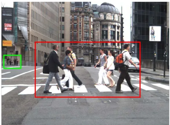
The pedestrian sizes in real world are different from each other. Besides the height diversity of different people, many imaging differences are incurred by the different distances between people and the camera. Figure 1 shows a high resolution corresponds to the large pedestrian scale and a low resolution corres-ponds to the small pedestrian scale in the process of pedestrian detection.

Pedestrians contain rich information in the case of high resolution [6], and it is more likely for them to be detected. Even if they are locally overlapped, many algorithms have the capability to detect these targets [7]. However, in the case low resolution, the pedestrians which contain a small amount of information cannot be detected easily. Meanwhile, low resolution pedestrians are very vul-nerable to the interferences of the surrounding environments. In most cases, a de-tection algorithm has a much better dede-tection result for the high resolution pede-strians than that for the low resolution pedepede-strians. Dalal and Triggs [8] proposed a HOG detector. If the detection window is fixed to 128×64 pixels during

training and detection, this detector can generate good effects at the time of de-tecting pedestrians with pixels greater than 128×64. However, when the target

pedestrians are smaller than 128×64, the detector almost fails to detect any

pe-destrian. Although the target can be increased to larger than 128×64 pixels by

means of interpolation, the detection accuracy is still brought down. The DPM pedestrian detector makes use of a root filter and several part filters to describe the pedestrians. Information in the pedestrians of high resolution is sufficient.

Figure 2(a) and Figure 2(b) are results obtained by utilizing a standard DPM

[image:2.595.230.516.502.712.2]

[image:3.595.210.533.62.206.2]

(a) (b)

Figure 2.The detection result of standard DPM. (a) The part filter and root filter in DPM (b) The detection result of standard DPM.

detector to detect pedestrians in Figure 1. It is obvious that the small-scale pe-destrians cannot be detected successfully. Therefore, the overall detection effect can be improved if we can improve the detection effect for low resolution pede-strians and prevent affecting the detection effect for high resolution pedepede-strians. In this paper, we propose a multi-resolution DPM pedestrian detection algo-rithm, which takes advantage of the standard DPM framework in training the pedestrian with the resolution factor as a hidden variable. For the high resolu-tion pedestrians, the response can be figured out in the first place. And its loca-tion can be estimated with the combinaloca-tion of this high resoluloca-tion response and the response under a corresponding low resolution. However, for the low resolu-tion pedestrians, the judgment over possible locaresolu-tions of these targets is carried out by only calculating the responses under the low resolution. High resolution and low resolution are only intuitive concepts in the common sense. In addition, resolution is closely associated with the heights of pedestrian samples.

Structure of this paper is as follows. In section 2, we thoroughly illustrate the DPM model for pedestrian detection, depicts the DPM learning algorithm, and describe the parameter initialization and the training procedures. In section 3, we illustrate the improved DPM algorithm in case of multi-resolution targets, by analyzing the features of pedestrian detection under multi-resolution, and de-scribing the improved multi-resolution DPM pedestrian detection algorithm in detail. In Section 4, we apply this improved algorithm to a general dataset to comparatively analyze the experimental results.

2. Overview of Related Theory

2.1. Deformable Part Model

The DPM pedestrian detection is a x-resolution detection method. However, to some extent the algorithm is able to adapt to different resolutions, because of the following three reasons.

Firstly, the DPM features are based on the image pyramid HOG features [11], which are adaptable to the scale variation within a certain range. Secondly, be-cause the available data sets often consist of a large number of pedestrian sam-ples, we have enough information for training a DPM model. For example, over 84% positive samples in the Caltech pedestrian database are over 30 pixels in height, over 16% positive samples are more than 80 pixels in height, and around 69% positive samples are between 30 pixels and 80 pixels in height.

2.2. Hard Example Mining (SVM)

In the training procedure, there are usually more negative samples than the available positive samples. Taking pedestrian detection for example, the images of pedestrians are positive samples, and the images without pedestrian are nega-tive samples. In this case, 105 _{samples can be generated from an image, most of} which are negative samples. It is almost impossible to take all negative samples into consideration. Therefore, we select the positive samples and the hard exam-ples for constructing a training set. The hard examexam-ples are referred to those which are incorrectly classified at the first time. The Bootstrapping classification algorithm is employed for training an initial negative sample set. The algorithm collects the incorrectly classified samples at the first time, add these samples to the negative sample set to form the hard samples. The process is repeated for several times until a good classification result is achieved. We define the hard example and easy sample as follows:

(

,

) (

{

,

)

|

( )

1

}

H β D = x y ∈D yfβ x < (1)

(

,

) (

{

,

)

|

( )

1

}

E β D = x y ∈D yfβ x > (2)

where, H

(

β

,D

)

denotes the incorrectly classified samples at the first time or the samples located within the classification boundary E

(

β

,D

)

denote the correctly classified samples. The samples on the classification boundary do not belong to H

(

β

,D

)

or E

(

β

,D

)

. *

( )

_{arg min}

( )

D

D _βL

β = β _.

Because LD is strictly convex,

( )

* _D

β is the single result of the optimized problem. Given a sample library D, we want to find a small sample set C with C⊆D and β*

( )

C =β*

( )

D . To solve this problem, we firstly define an initial

set which contains all the training samples. We train an LSVM model, and renew the previous set by removing the simple samples and by adding the new hard examples.

2.3. Hard Example Mining with LSVM

For the LSVM, mining hard examples is equivalent to optimize _{( )( )}

p

Z

D _β rather than LD

( )

β

. This constraint turns the whole optimization problem to a convex

As for the hard example mining with SVM, we define an set with samples in the form of

( )

x z, , in which z∈Z x

( )

. In the real application, the set consists of Φ

( )

x z, rather than

( )

x z, . We define a vector set F= ⋅

( )

i v , in which i denotes sample index, and v= Φ

( )

x z, with z∈Z x

( )

i . Because the hidden

variable z is not fixed, for each sample x_i, there may be multiple correspond-ing

( )

i v, ∈F. Then we define I F

( )

as the index of vectors in the vector set

F, and dene the target function for

β

with the feature vectors in F:

( )

( )

(

(

( )

)

)

2

,

1

max 0,1 max

2

F i I F i i v F

L β = β +C

∑

∈ −y ∈ β⋅v (3)

F

L can be optimized with the gradient-descent algorithm. We use V i

( )

as the set of feature factors v.

The gradient-descent algorithm is described as follows. 1. at is the learning rate for iteration t.

2. i∈I F

( )

is the index for samples in F. 3. vi =arg maxv V i∈( )β⋅v.

4. If yi

( )

β

vi ≥1, then

β β

= −at

( )

β

.

5. Otherwise,

β β

= −at

(

β

−Cny vi i

)

.

We set *

( )

( )

arg min _F

F _βL

β = β _{and try to find} *

( )

*

(

( )

)

p

F

D Z

β

=

β

_{in a}

sample set D Z

( )

p of small size.

As for the hard example mining with standard SVM, we define the feature vectors for hard and simple example in training set D as follows.

(

,

)

{

(

,

(

, _i

)

)

| _i arg max

(

_i,

)

and _i

(

(

_i, _i

)

)

1

}

z z

H β D i x z z β x z y β x z

∈

= Φ = ⋅ Φ ⋅ Φ <

(

,

) ( )

{

, | i

(

)

1

}

E β F = i v ∈F y β⋅v > (4)

We find the hard examples by calculating *

(

( )

)

p

D Z

β

_. F₁ is defined as the initial feature vector set.

The LSVM hard example mining algorithm is given below: 1. Train model with *

( )

:

t Ft

β =β _.

2. If

H

(

β

,

D Z

( )

_p

)

⊆

F

_t, stop the iteration and return β_t.

3. Remove the simple samples by Ft′:=Ft\X , where X ⊆E

(

β

t,Ft

)

.

4. Add new hard examples by Ft+1:=FtX , where

( )

(

_t

,

_p

)

\

_t

X



H

β

D Z

F

≠ ∅

.

In the 3rd step simple samples are removed from the training set, while in the 4th step new hard examples are added to the training set. The entire iteration procedure terminates when there are no hard examples to add.

3. Pedestrian Detection with Multi-Resolution DPM

3.1. Fixed Resolution Model

Let x represent an image window, and ∅

( )

x represent the image feature. As many slide window detection algorithms, we have

( )

0 where

( )

( )

f x > f x = ⋅∅w x (5)

and negative samples of the training set

(

x y_i, _i

)

, in which y_i∈ −

{ }

1,1 . The

commonly available training algorithms include SVM and boosting, and we em-ploy the linear SVM for training the parameter w:

( )

(

)

1

arg min max 0,1

2

i

w i i i

w = w w C⋅ +

∑

−y w⋅∅ x (6)

in which xi is assumed to be of a fixed size during training and testing. We

de-fine a feature vector ∅

( )

x to deal with the windows of different sizes.

3.2. Models with Fixed Resolutions

If an image contains objects of different resolutions at the same time, the detec-tor of a fixed resolution usually cannot detect all different objects simultaneous-ly. Because we can describe the different distances of pedestrians in an image, for each window x we can dene a binary variable s to represent the distance of a pedestrian. We use s=0 to represent the distant target pedestrians, and use

1

s= to denote the close target pedestrian. Our classifier is the same as the

pre-vious one. f x s

( )

, = ⋅∅w

( )

x s, ,

( )

( )

( )

_{( )}

0 1 0 0 1

, if 0 and , if 1

0

1 0

x

x s s x s s

x ∅             ∅ = = ∅ = =   ∅          (7)

where ∅0

( )

x and ∅1

( )

x denote the features at different scales, such as a pedestrian of 50 pixels and a pedestrian of 100 pixels.

3.3. Multi-Scale Multi-Resolution Model

For the close target pedestrians with s = 1, we can transform a model for high- resolution targets to two models for different resolution targets. For instance, we can transform a 100 pixels window into two windows of 50 pixels, and calculate the features at the small window scale. In this way, we can transform a model for high-resolution target to two models for different resolution targets:

(

)

( )

(

)

( )

( )

1 0 1 1 0

, , if 0 and , , if 1

0

0 1

x x

x s z s x s z s

x ∅ ∅             ∅ = = ∅ = =   ∅          (8)

With the above formula we can transform the object features at a fixed resolu-tion into features at different resoluresolu-tions. However, because ∅0

( )

x is different at different resolutions, the linear SVM is not suitable for training models.

but not invariant to the 100 pixels height pedestrians. If we are to detect a large- scale target, we can choose a low-resolution template. And if we hope to gain more information, we can select a high-resolution template. For a good adapta-bility to the deformation at a large scale, we adopt a DPM model. As a hidden parameter z is defined in the DPM model, we use ∅1

( )

x z, as the combina-tion of HOG feature and the deviacombina-tion.

(

)

( )

(

)

( )

( )

0 0 0 1 1

, , if 0 and , , if 1

0 ,

0 0

x x

x s z s x s z s

x z ∅ ∅             ∅ =_{ } = ∅ =_{ } = ∅         (9)

The classifier passes through all the hidden variables at last, and calculates

( )

, maxz

(

, ,

)

f x s = w⋅∅ x s z :

( )

0 0

( )

_{( )}

0

_{( )}

0 0 1 1

if 0 ,

maxz , if 1

w x b s

f x s

w x x z b s

∅ + =



=  ⋅_{⋅∅ + ⋅∅ + =}

 (10)

( )

,

f x s is transformed into a standard linear template for calculating the re-sponse at a low resolution. For calculating the rere-sponse at a high resolution,

( )

f x would need to search all part models to nd the model which makes the maximum response. Suppose the distances between different parts and the root filter are independent from each other, the following formula can be calculated with the

QP

algorithm:

(

)

(

)

(

)

1 1 ,

maxzw⋅∅ x z, =maxz

∑

jwj⋅∅ x z, j +

∑

j k E∈ wjk⋅∅ zj,zk (11)

in which zj denotes the location of part

j

, wj denotes the template of part

j

, w_kj denotes the deformable model of part

j

and k, and E denotes the boundary. ∅

(

x z, _j

)

represents the HOG feature at location z_j , and

(

z z_j, _k

)

∅ represents the deformation difference between part

j

and part k.

For a given training set

(

x s y_i, ,_{i i}

)

, we can employ the LSVM algorithm for

training the model parameter w.

At the stage of model training, we set si =1 if the training sample has a large

scale

(

h>0

)

, in which s_i is no longer a hidden variable. And we set si=0 if

the training sample has a small scale

(

h<50

)

, in which s_i is not a hidden va-riable, either. If the training sample has a medium scale

(

50< <h 100

)

, the

training sample can be considered as both a high resolution object and a low resolution object. In this case, si becomes a hidden variable, which can be

added to the set of hidden variables of the LSVM model for training. The rough procedure consists of the random initialization of variables si and zi, the

cal-culation of model parameter

β

_{in model training, and the acquisition of value} for the hidden variable in accordance to the maximum response which would be taken into the next iteration.

4. Experiment Process and Dataset

4.1. Overview of the Algorithm

with two target models. But there are also big differences between these me-thods. Firstly, many parameters are shared in our deformable model, while all parameters in the hybrid deformable model are independent from each other. Secondly, our multi-resolution deformable model consist a different procedure for the variable si. At the training state, si is a hidden variable, while at the

test state si would become a visible variable. The procedure of pedestrian

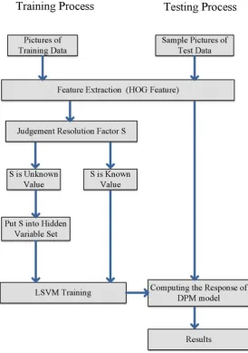
de-tection by multi-resolution DPM is shown in Figure 3.

First, DPM parameters w0 and w1 are initialized by the initialization me-thod as illustrated before. w0 is the model parameter at a low resolution, while

1

w is the model parameter at a high resolution. At the training state, we set the value of s by considering the height h of a trained sample, for which s=1

if h>100 and s=0 if h<50. For the samples with s=1, LSVM can be

used to train a standard DPM model, which renders the model parameter w1. For the samples with s=1, a linear SVM can be used to train a DPM model (no

[image:8.595.234.509.325.715.2]

hidden variable is involved), which renders the model parameter w0. For the samples with height 50<h<100, we add s to the set of hidden variables, and

train the model with the LSVM algorithm.

4.2. Evaluation Method

Whole Image Evaluation

The detection result for an image consist of a set of bounding boxes

( )

BB and a corresponding confidence score [13]. If the detection result

(

BBdt

)

and

the standard result

(

BBgt

)

has a great extent of overlapping, we consider the detection result matches the standard result. We define that a detection result matches the standard result if they have over 50% parts overlapped:

(

)

(

)

0 0.5

dt gt dt gt

area BB BB a

area BB BB

=  >

 (12)

Each

(

BBdt

)

can match to at most one

(

BBgt

)

, which means that every de-tected

(

BBdt

)

can only match one

(

BBgt

)

but not multiple

(

BBgts

)

. There-fore, if a detection result

(

BBdt

)

could match multiple

(

BBgts

)

we only select the

(

BBgt

)

with the highest confidence as the final detection result. If a

(

BBdt

)

is not matched with any

(

BBgt

)

, it is labeled as false positive. And if a

(

BBgt

)

is not matched with any

(

BBdt

)

, it is labeled as false negatives as well.

4.3. Experiment Dataset

1. INRIA

The INRIA data set is a static pedestrian detection database which has been widely employed in recent researches. The training set consists of 614 positive samples (containing 2416 pedestrians) and 1218 negative samples. The test set consists of 288 positive samples (containing 1126 pedestrians) and 453 negative samples. Images in the INRIA data set are mainly collected from google, GRAZ- 01 and personal photographs.

2.Caltech Pedestrian Database

The Caltech Pedestrian Database is a large scale database. It consists of videos of 640 × 480 pixel with 30 frames per second, captured by in-vehicle cameras for about 10 hours. Within these videos, 250,000 frames (around 137 minutes), 350,000 bounding boxes, and 2300 pedestrians are manually annotated by hu-man experts. The data set is divided into 10 sets, among which sets 00 - 05 are used for training, and sets 06 - 10 are used for testing. In our experiment, we also employ sets 00 - 05 for training and sets 06-10 for testing.

Pillor [14] divide samples in the Caltech Pedestrian Library into distant

(

h<30

)

, medium

(

30< <h 80

)

and near h>80 types, according to the

heights

( )

h of pedestrians.

The model feature of DPM is based on the HOG feature of the image pyra-mid, and DPM has good adaptability to a certain range of scale changes. Usually the pedestrian samples in our data set are not too small, so there is enough in-formation for building the DPM model.

more than 16% of the positive samples have height greater than 80 pixels, and about 69% of the positive samples have height from 30 to 80 pixels. In the case of high-resolution

(

h>100

)

, the DPM model show very good results in

tradition-al DPM model tests. In this work we defined targets with height h>100 as the

high resolution target, targets with height h<50 as the low resolution targets,

and targets with height 50<h<100 as the unknown resolution targets in

which case the resolution factor is treated as a hidden variable.

5. Results and Discuss

5.1. The Result in INRIA

There are nearly one thousand pictures in INRIA pedestrian database. Our model is trained on the INRIA training set, and evaluated on the INRIA test set. The multi-resolution DPM-based pedestrian detection algorithm acquires a pre-cision of 87.2% on INRIA pedestrian database, which is slightly better than 86.9% as the precision of the standard DPM. This is mainly because that there are too few picture samples in this data set, and the pedestrian scale is too big in the pictures. Only a few pictures contain the small-scale pedestrians, in which case the multi-resolution DPM detector cannot change the detection method at the high resolution. Therefore, the detection result is almost the same as the standard DPM result.

5.2. The Result in Caltech Database

Training our model on the Caltech pedestrian database is more challenging than on the INRIA dataset. The number of samples in the Caltech pedestrian dataset is large, which is much larger than the number of samples in the INRIA dataset. The Caltech pedestrian dataset consists samples of 640×480 pixel resolution,

in which many pedestrian targets of small scales are included.

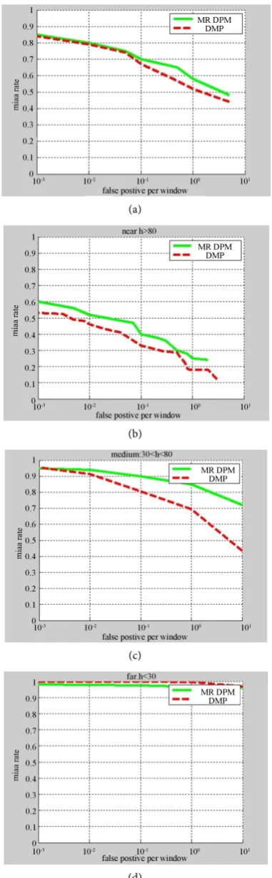
In this section, set0 to set5 in Caltech database are employed for training, and set6 to set11 are chosen for testing. Figures 4(a)-(d) show the detection results for all-distance, near-distance, middle-distance and far-distance samples, respec-tively. Specifically, the near-distance corresponds to pedestrians with height

80

h> pixel, the middle-distance corresponds to pedestrians with height

30

h> but h<80, and the far-distance corresponds to pedestrian with height 30

h< .

The experiment result suggests that the multi-resolution DPM algorithm renders better detection results than that the standard DPM in terms of all test-ing sets, Figure 4(a) shows the result based on all test samples. The multi-reso- lution DPM-based pedestrian detection algorithm achieves a missing rate of 52% (1FPPI), which is much better than the missing rate 59% (1FPPI) achieved by the DPM pedestrian detection algorithm. This result suggesting that multi-reso- lution DPM has better detection effect than the standard DPM. In terms of the large-scale samples (h>80) in Caltech database, the multi-resolution DPM-

[image:11.595.278.469.70.687.2]

which suggests that the multi-resolution DPM also outperforms the standard DPM for large-scale targets. For small-scale samples, the difference in both models is not as obvious as shown in Figure 4(b), which is mainly because, that the useful information at small scales is very limited (the objects at less than 30 pixels are known as small-scale objects). At this point, the detection algorithm cannot acquire enough information for detection.

5.3. The Result in Part of Caltech Database

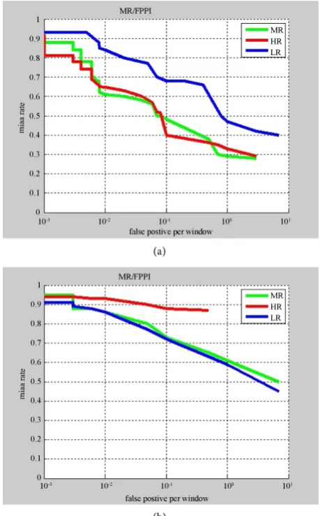
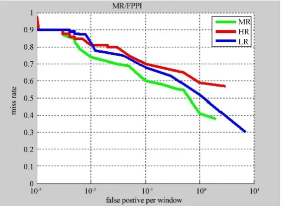
In order to better explain the experiment result, we further select 3000 pictures from the standard Caltech database for evaluation. This experiment is conducted to compare the detection effects of the detection algorithm at a high resolution (corresponding to the standard DPM algorithm), the detection algorithm at a low resolution (corresponding to merely the root filter-based DPM algorithm), and the proposed multi-resolution DPM algorithm.

[image:12.595.258.488.325.695.2]

The experiment result is shown in Figure 5, in which LR represents the low- resolution detection algorithm, HR represents the high-resolution detection al-

gorithm, and MR represents the multi-resolution detection algorithm.

The results of large-scale target

(

h>90

)

detection as shown in Figure 5(a),

the multi-resolution DPM algorithm achieves similar performance as the stan-dard DPM algorithm. Both algorithms are better than the low-resolution detec-tor.

Figure 5(b) shows the terms of the small-scale target

(

h<90

)

detection, we

find that the detection effect of the standard DPM algorithm drops quickly as the target scale grows small. The detection effect of the multi-resolution DPM algorithm is slightly lower than that of the rigid template.

According to the overall comparison is shown in Figure 6, the multi-resolu- tion DPM algorithm is better than the high-resolution detection algorithm on the testing set. We find that the missing rate on test set is 52% with a rigid tem-plate. This is lower than 59%, which is the missing rate with the standard DPM algorithm. This is because most of the pedestrian samples are with height

30<h<80, and even the high-resolution algorithm cannot detect the small-

scale targets. The standard DPM algorithm achieves a good detection effect for the large-scale targets.

6. Conclusion

[image:13.595.232.515.507.714.2]

In this paper we proposed a Pedestrian Detection Method at Multiple Resolu-tion. Especially during pedestrian detection under the high resolution, such an algorithm can generate very significant effects. However, targets in images ac-quired in the real world are under diverse resolutions in most cases. Considering this, the standard DPM is subjected to great limitations. Here, a multi-resolution DPM algorithm based on the standard DPM algorithm is presented. In this way, pedestrian detection is fixed to different resolutions. For example, pedestrians under the high resolution can be detected through a deformable part model, while those under the low resolution are detected based on the rigid template. In

Caltech, omission ratio of a multi-resolution DPM detector was 52% (1FPPI); comparatively, it became 59% (1FPPI) as far as a standard DPM detector was concerned. In the large-scale sample set of Caltech, omission ratio of the multi- resolution and the standard DPM detectors were 18% (1FPPI) and 26% (1FPPI) respectively. The general results of proposed method are better than the stan-dard DPM.

Acknowledgements

This research was partially supported by JSPS KAKENHI Grant Numbers 15K00425, 15K00309.

References

[1] Markus, E. and Gavrila, D.M. (2009) Monocular Pedestrian Detection: Survey and Experiments. IEEE Transactions on Pattern Analysis and Machine Intelligence, 31, 2179-2195. https://doi.org/10.1109/TPAMI.2008.260

[2] Bagheri, M., Siekkinen, M. and Nurminen, J.K. (2016) Cloud-Based Pedestrian Road-Safety with Situation-Adaptive Energy-Efficient Communication. IEEE Intel-ligent Transportation Systems Magazine, 8, 45-62.

https://doi.org/10.1109/MITS.2016.2573338

[3] Guo, A., Xu, M., Ran, F., et al. (2016) A Real-Time Pedestrian Detection System in Street Scene. International Journal on Smart Sensing and Intelligent Systems, 9, 1592-1613.

[4] Zhe, L. and Davis, L.S. (2010) Shape-Based Human Detection and Segmentation via Hierarchical Part-Template Matching. IEEE Transactions on Pattern Analysis and Machine Intelligence, 32, 604-618. https://doi.org/10.1109/TPAMI.2009.204

[5] Zhe, L., Hua, G. and Davis, L.S. (2009) Multiple Instance Feature for Robust Part-Based Object Detection. IEEE Conference on Computer Vision and Pattern Recognition (CVPR 2009),Miami,20-25 June 2009.

[6] Liu, Y., Lasang, P., Siegel, M., et al. (2016) Multi-Sparse Descriptor: A Scale Inva-riant Feature for Pedestrian Detection. Neurocomputing, 184, 55-65.

https://doi.org/10.1016/j.neucom.2015.07.143

[7] An, M.S. and Kang, D.S. (2015) A Method of Robust Pedestrian Tracking in Video Sequences Based on Interest Point Description. International Journal of Multimedia and Ubiquitous Engineering, 10, 35-46.

https://doi.org/10.14257/ijmue.2015.10.10.04

[8] Navneet, D. and Triggs, B. (2005) Histograms of Oriented Gradients for Human Detection. 2005 IEEE Computer Society Conference on Computer Vision and Pat-tern Recognition (CVPR’05), San Diego, 20-25 June 2005.

[9] Afsar, P., Cortez, P. and Santos, H. (2015) Automatic Visual Detection of Human Behavior: A Review from 2000 to 2014. Expert Systems with Applications, 42, 6935-6956. https://doi.org/10.1016/j.eswa.2015.05.023

[10] Kim, S. and Cho, K. (2015) Design of High-Performance HOG Feature Calculation Circuit for Real-Time Pedestrian Detection. Journal of Information Science and Engineering, 31, 2055-2073.

[11] Lin, C.F., Chen, C.S., Hwang, W.J., et al. (2015) Novel Outline Features for Pede-strian Detection System with Thermal Images. Pattern Recognition, 48, 3440-3450.

https://doi.org/10.1016/j.patcog.2015.04.024

Part-Based Models. IEEE Transactions on Pattern Analysis and Machine Intelli-gence, 32, 1627-1645. https://doi.org/10.1109/TPAMI.2009.167

[13] Piotr, D., et al. (2012) Pedestrian Detection: An Evaluation of the State of the Art. IEEE Transactions on Pattern Analysis and Machine Intelligence, 34, 743-761.

https://doi.org/10.1109/TPAMI.2011.155

[14] Piotr, D., Belongie, S. and Perona, P. (2010) The Fastest Pedestrian Detector in the West. BMVC, 2.

Submit or recommend next manuscript to SCIRP and we will provide best service for you:

Accepting pre-submission inquiries through Email, Facebook, LinkedIn, Twitter, etc. A wide selection of journals (inclusive of 9 subjects, more than 200 journals)

Providing 24-hour high-quality service User-friendly online submission system Fair and swift peer-review system

Efficient typesetting and proofreading procedure

Display of the result of downloads and visits, as well as the number of cited articles Maximum dissemination of your research work

Submit your manuscript at: http://papersubmission.scirp.org/