http://www.scirp.org/journal/am ISSN Online: 2152-7393
ISSN Print: 2152-7385
Analytical Solution for the Time-Dependent
Emden-Fowler Type of Equations by Homotopy
Analysis Method with Genetic Algorithm
Waleed Al-Hayani
1, Laheeb Alzubaidy
2, Ahmed Entesar
11Department of Mathematics, College of Computer Science and Mathematics, University of Mosul, Mosul, Iraq 2Department of Software Engineering, College of Computer Science and Mathematics, University of Mosul, Mosul, Iraq
Abstract
In this paper, Homotopy Analysis method with Genetic Algorithm is pre-sented and used to obtain an analytical solution for the time-dependent Em-den-Fowler type of equations and wave-type equation with singular behavior at x = 0. The advantage of this single global method employed to present a re-liable framework is utilized to overcome the singularity behavior at the point x
= 0 for both models. The method is demonstrated for a variety of problems in one and higher dimensional spaces where approximate-exact solutions are obtained. The results obtained in all cases show the reliability and the effi-ciency of this method.
Keywords
Homotopy Analysis Method, Genetic Algorithm, Emden-Fowler Equation, Wave-Type Equation, Adomian Polynomials, Noise Terms, Padé
Approximants, Simpson Rule
1. Introduction
In many previous works of the diffusion of heat perpendicular to the surfaces of parallel planes are modeled by the heat equation
( )
( ) ( ) ( )
, , , 0 , 0 , 0,r r
x t
x
x− x y +af x t g y +h x t = y < ≤x L < <t T r> (1)
or equivalently
( ) ( ) ( )
, , , 0 , 0 , 0,xx x t
r
y y af x t g y h x t y x L t T r
x
+ + + = < ≤ < < > (2)
where f x t g y
( ) ( ) ( )
, +h x t, is the nonlinear heat source, y x t( )
, is the tem-How to cite this paper: Al-Hayani, W.,Alzubaidy, L. and Entesar, A. (2017) Analyt-ical Solution for the Time-Dependent Em-den-Fowler Type of Equations by Homotopy Analysis Method with Genetic Algorithm. Applied Mathematics, 8, 693-711.
https://doi.org/10.4236/am.2017.85055
Received: December 30, 2016 Accepted: May 22, 2017 Published: May 25, 2017
Copyright © 2017 by authors and Scientific Research Publishing Inc. This work is licensed under the Creative Commons Attribution International License (CC BY 4.0).
http://creativecommons.org/licenses/by/4.0/
perature, and t is the dimensionless time variable. For the steady-state case, and for r=2, h x t
( )
, =0, Equation (2) is the Emden-Fowler equation [1] [2] [3]given by
( ) ( )
( )
0( )
2
0, 0 , 0 0,
y y af x g y y y y
x
′′+ ′+ = = ′ = (3)
where f x
( )
and g y( )
are some given functions of x and y respectively. For( )
1f x = and g y
( )
=yn, Equation (3) is the standard Lane-Emden equationthat was used to model the thermal behavior of a spherical cloud of gas acting under the mutual attraction of its molecules [1] and subject to the classical laws of thermodynamics. For other special forms of g y
( )
, the well-known Lane-Emden equation was used to model several phenomena in mathematical physics and astrophysics such as the theory of stellar structure, the thermal behavior of a spherical cloud of gas, isothermal gas spheres, and theory of thermionic currents
[1][2][3]. A substantial amount of work has been done on this type of problems for various structures of g y
( )
in [1]-[7].On the other hand, the wave type of equations with singular behavior is given by
( )
( ) ( ) ( )
, , , 0 , 0 , 0,r r
x tt
x
x− x y +af x t g y +h x t =y < ≤x L < <t T r> (4)
or equivalently
( ) ( ) ( )
, , , 0 , 0 , 0,xx x tt
r
y y af x t g y h x t y x L t T r
x
+ + + = < ≤ < < > (5)
will be examined as well, where f x t g y
( ) ( ) ( )
, +h x t, is a nonlinear source, t isthe dimensionless time variable, and y x t
( )
, is the displacement of the wave atthe position x and at time t. The singularity behavior that occurs at the point
0
x= is the main difficulty in the analysis of Equations (2) and (5). Wazwaz [8]
used the Adomian decomposition method (ADM) to get an analytical solution for the time-dependent Emden-Fowler type of equations and wave-type equa-tion with singular behavior.
The main objective of this paper is to apply Homotopy Analysis Method (HAM) to obtain approximate-exact solutions for different models for the time- dependent Emden-Fowler type of equations and wave-type equation with singu-lar behavior at x=0. While the VIM [9][10] requires the determination of
La-grange multiplier in its computational algorithm, HAM is independent of any such requirements, HAM handles linear and nonlinear terms in a simple and straightforward manner without any additional requirements. Also, in this paper we apply Genetic Algorithm (GA) to obtain an approximate solution of the same equations.
In what follows, we give a brief review of Homotopy analysis method and Ge-netic algorith.
2. Analysis of the Homotopy Analysis Method
equation:
( )
,( )
, ,N y x t =k x t (6)
where N is a nonlinear operator, x and t denote the independent variables,
( )
,y x t is an unknown function and k x t
( )
, is a known analytic function. Forsimplicity, we ignore all boundary or initial conditions, which can be treated in the similar way. By means of generalizing the traditional Homotopy method, Liao [11] constructs the so called zero-order deformation equation
(
1−q L)
φ(
x t q, ;)
−y0( )
x t, =qh N φ(
x t q, ;)
−k x t( )
, , (7) where q∈[ ]
0,1 is an embedding parameter, h is a nonzero auxiliary parameter, L is an auxiliary linear operator, y0( )
x t, is an initial guess of y x t( )
, and(
x t q, ;)
φ is an unknown function. It is important, that one has great freedom to choose auxiliary objects such as h and L in HAM. Obviously, when q=0 and
1
q= it holds
(
x t, ; 0)
y0( )
x t, ,(
x t, ;1)
y x t( )
, ,φ = φ = (8)
respectively. Thus, as q increases from 0 to 1, the solution φ
(
x t q, ;)
varies fromthe initial guess y0
( )
x t, to the solution y x t( )
, . Expanding φ(
x t q, ;)
in Taylor series with respect to q, we have(
)
0( )
( )
1
, ; , m , m,
m
x t q y x t y x t q
φ +∞
=
= +
∑
(9)where
( )
(
)
0
, ; 1
, .
!
m
m m
q
x t q y x t
m q
φ
=
∂ =
∂ (10)
If the auxiliary linear operator, the initial guess, the auxiliary parameter h, and the auxiliary function are so properly chosen, the above series (9) converges at
1,
q= then we have
(
)
0( )
( )
1
, ;1 , m , ,
m
x t y x t y x t
φ +∞
=
= +
∑
(11)which must be one of the solutions of the original nonlinear equation, as proved by Liao [11]. If h= −1, Equation (7) becomes
(
1−q L)
φ(
x t q, ;)
−y0( )
x t, +q N φ(
x t q, ;)
−k x t( )
, =0, (12) which is used mostly in the Homotopy perturbation method [12].According to Equation (10), the governing equation can be deduced from the zero-order deformation Equation (7). We define the vectors
( ) ( )
( )
{
0 , , 1 , , , ,}
. i= y x t y x t y x tiy (13)
Differentiating Equation (7) m times with respect to the embedding parameter
q and then setting q=0 and finally dividing them by m!, we have the so-
called mth-order deformation equation
( )
, 1( )
,(
1)
,m m m m m
where
(
1) ( )
1{
(
1)
( )
}
0, ; ,
1
, 1 !
m
m m m
q
N x t q k x t
R
m q
φ
−
− −
=
∂ − =
− ∂
x (15)
and
0, 1,
1, 1.
m
m m χ = ≤>
(16)
It should be emphasized that ym
( )
x t,(
m≥1)
are governed by the linearEquation (14) with the linear boundary conditions that come from the original problem, which can be easily solved by symbolic computation softwares such as Maple and Mathematica.
3. Genetic Algorithms
Definition 1 Genetic Algorithms are search and optimization techniques based on Darwin’s Principle of Natural Selection.
Definition 2 Genetic Algorithm Operators [13][14]
The simplest form of genetic algorithm involves three types of operators: se-lection, crossover and mutation.
Selection: This operator selects chromosomes in the population for reproduc-tion. The fitter the chromosome, the more times it is likely to be selected to re-produce.
Crossover: This operator randomly chooses a locus and exchanges the sub-sequences before and after that locus between two chromosomes to create two offspring. For example, the strings 10000100 and 11111111 could be crossed over after the third locus in each to produce the two offspring 10011111 and 11100100.
The crossover operator roughly mimics biological recombination between two single-chromosome (haploid) organisms.
Mutation: This operator randomly flips some of the bits in a chromosome. For example, the string 00000100 might be mutated in its second position to yield 01000100. Mutation can occur at each bit position in a string with some probability, usually very small (e.g., 0.001).
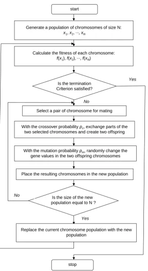
Algorithm 3 A Simple Genetic Algorithm [13][14]
Given a clearly defined problem to be solved and a bit string representation for candidate solutions, a simple GA works as follows:
1. Start with a randomly generated population of n l-bit chromosomes (can-didate solutions to a problem).
2. Calculate the fitness f x t
( )
, of each chromosome x and t in thepopula-tion.
3. Repeat the following steps until n offspring have been created:
than once to become a parent.
(b) With probability pc (the “crossover probability” or “crossover rate”), cross over the pair at randomly chosen point (chosen with uniform probability) to form two offspring. If no crossover takes place, form two offspring that are exact copies of their respective parents. (Note that here the crossover rate is defined to be the probability that two parents will crossover in a single point. There are also “multi-point crossover” versions of the GA in which the crossover rate for a pair of parents is the number of points at which a crossover takes place).
(c) Mutate the two offspring at each locus with probability pm (the “mutation probability” or “mutation rate”), and place the resulting chromosomes in the new population. If n is odd, one new population member can be discarded at random.
4. Replace the current population with the new population. 5. Go to step 2.
Also see the flow chart (Figure 1).
4. Applications of the Method
In this work, we examine six distinct models with singular behavior at x=0,
two linear time-dependent Lane-Emden type of equations, two linear models of wave-type equation, and two nonlinear singular models. To show the high accu-racy of the solution results compared with the exact solution, we give the nu-merical results applying the Genetic Algorithm (GA), HAM
(
n=5)
, Padéap-proximants (PA) of order
[
p q]
, and the numerical solution with the Simpsonrule (SIMP). Twenty points have been used in the Simpson rule. The computa-tions associated with the examples were performed using a Maple 13 package with a precision of 20 dgits.
4.1. Time-Dependent Lane-Emden Type
Example 1. Firstly, let us consider the following linear homogeneous equation
(
2)
2
6 4 cos ,
xx x t
y y x t y y
x
+ − + − = (17)
subject to initial conditions
( )
sin( )
0, e t, x 0, 0.
y t = y t = (18)
To solve Equations (17)-(18) by means of the standard HAM, we choose the initial approximation
( )
sin0 , e ,
t
y x t = (19)
and the linear operator
(
)
2(
2)
(
)
, ; 2 , ;
, ; x t q x t q ,
L x t q
x x
x
φ φ
φ =∂ + ∂
∂ ∂ (20)
with the property
1
2 0,
c
L c
x
− + =
Figure 1. Flow Chart of Genetic Algorithm.
where ci
(
i=1, 2)
are constants of integration. Furthermore, Equation (17)suggests that we define the nonlinear operator as
(
)
(
)
(
)
(
)
(
)
(
)
2
2
2
, ; 2 , ;
, ;
, ;
6 4 cos , ; .
x t q x t q N x t q
x x
x
x t q x t x t q
t
φ φ
φ
φ φ
∂ ∂
= +
∂ ∂
∂
− + − −
∂
(22)
Using the above definition, we construct the zeroth-order deformation
equa-start
Generate a population of chromosomes of size N:
x1, x2,···,xN
Calculate the fitness of each chromosome:
f(x1), f(x2),···,f(xN)
Is the termination Crlterion satisfied?
Select a pair of chromosome for mating
With the crossover probability pc, exchange parts of the
two selected chromosomes and create two offspring
With the mutation probability pm, randomly change the
gene values in the two offspring chromosomes
Place the resulting chromosomes in the new population
Is the size of the new population equal to N ?
Replace the current chromosome population with the new population
stop
Yes
No
No
tion as in (7) and (8) and the mth-order deformation equation for m≥1 is
( )
, 1( )
,(
1)
,m m m m m
L y x t −χ y − x t =hR y − (23)
with the initial conditions
( )
0, 0,( )
( )
0, 0m m x
y t = y t = (24)
where
(
) (
)
(
)
(
2)
(
)
1 1 1 1 1
2
6 4 cos .
m m m xx m x m m t
R y y x t y y
x
− = − + − − + − − − −
y (25)
Now, the solution of the mth-order deformation Equation (23) for m≥1 is
( )
( )
2 2(
)
1 0 0 1
, , x x .
m m m m m
y x t =χ y − x t +h x
∫ ∫
− x R y − (26)We now successively obtain
( )
( )
(
)
( )
(
) (
)
4 2 sin
1
2 8 2 6 2 4 2 2 sin
2
3 12 3 10 2 3 8 sin
3
2 3 6 2 3 4 2 3 2
1
, e ,
5
1 13 1 1
, e ,
90 105 5 10
1 59 1 1
, e
3510 11550 45 210
26 43 1
2 2
105 210 5
t
t
t
y x t hx hx
y x t h x h x h h x h h x
y x t h x h x h h x
h h x h h h x h h h x
= − −
= + − − − +
= − − + −
+ + − − − − + +
sin
e t,
(27)
and so on, in this manner the rest of the iterations can be obtained. Thus, the approximate solution in a series form is given by
( )
0( )
( )
1
, , m , ,
m
y x t y x t y x t
+∞
=
= +
∑
(28)Hence, the series solution when h= −1 is
( )
2 1 4 1 6 1 8 sin, 1 e .
2! 3! 4!
t
y x t = +x + x + x + x +
(29)
This series has the closed form as n→ ∞
( )
2 sin, ex t,
y x t = + (30)
which is the exact solution of (17)-(18) compatible with ADM [8]. Also, this example is solved by using GA as follows:
We’ll choose six values of x between
( )
0,1 randomly, and converting themfrom the decimal format to the binary format
1 1
0.2 0.001100110011
x t
=
2 2
0.3 0.010011001100
x t
=
3 3
0.5 0.100000 000000
x t
=
4 4
0.6 0.100110 011000
x t
5 5
0.8 0.110011001100
x t
=
6 6
0.9 0.111001100100
x t
=
that is,
i
x 0.001100 0.010011 0.100000 0.100110 0.110011 0.111001
i
t 0.110011 0.001100 0.000000 0.011000 0.011000 0.100100
Now,
i
x 0.1875 0.2969 0.5000 0.5938 0.7969 0.8906
i
t 0.7969 0.1875 0.0000 0.3750 0.1875 0.5625
( i,i)
f x t 2.1177 1.3159 1.2840 2.0521 2.2738 3.7675 ( i,i)
p x t 0.1653 0.1027 0.1002 0.1602 0.1775 0.2941
where f x t
(
i, i)
is the series solution of HAM given by (29) and p x t(
i,i)
=(
)
(
)
6 1
,
,
i i
i i i
f x t
f x t
=
∑
is the probability of each chromosomes with(
)
6
1 i,i 12.8110. i= f x t =
∑
We arrange the chromosomes an ascending order and then choose less than four chromosomes to find the best solution
31 31
21 21
41 41
11 11
0.100000, 0.000000
0.010011, 0.001100
0.100110, 0.011000
0.001100, 0.110011
x t
x t
x t
x t
= =
= =
= =
= =
In this step of GA, crossover operation (two points) is done as follows:
1 2
32 32
22 22
42 42
12 12
2, 5
0.100000, 0.001100 0.010011, 0.000000
0.101110, 0.010000 0.000100, 0.111011
cut cut
x t
x t
x t
x t
= =
= =
= =
= =
= =
In the last step of GA a mutation operation (bit inverse, m=3) and then
converting them from the binary format to the decimal format:
33 33
23 23
43 43
13 13
0.101000 0.6250, 0.000100 0.0625
0.011011 0.4219, 0.001000 0.1250
0.100110 0.5938, 0.011000 0.3750
0.001100 0.1875, 0.110011 0.7969
x t
x t
x t
x t
= = = =
= = = =
= = = =
= = = =
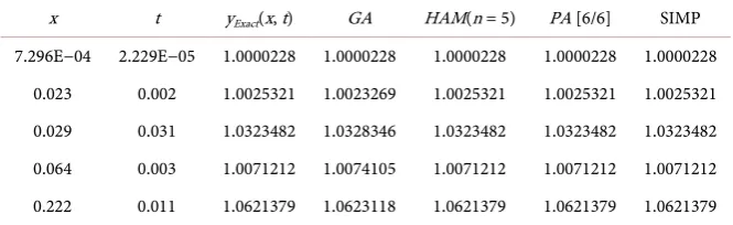
The optimal solution is found after 51 generation to converge to the exact so-lution, where x=7.2959306E−04 and t=2.2287430E−05. After execute
Table 1. Optimal solution of genetic algorithm for example 1.
x t yExact(x, t) GA HAM(n = 5) PA [6/6] SIMP
7.296E−04 2.229E−05 1.0000228 1.0000228 1.0000228 1.0000228 1.0000228 0.023 0.002 1.0025321 1.0023269 1.0025321 1.0025321 1.0025321 0.029 0.031 1.0323482 1.0328346 1.0323482 1.0323482 1.0323482 0.064 0.003 1.0071212 1.0074105 1.0071212 1.0071212 1.0071212 0.222 0.011 1.0621379 1.0623118 1.0621379 1.0621379 1.0621379
Example 2. We consider the following linear inhomogeneous equation,
(
2)
2 42
5 4 6 5 4 ,
xx x t
y y x y y x x
x
+ − + = + − − (31)
subject to initial conditions
( )
0, e ,t( )
0, 0.x
y t = y t = (32)
To solve Equations (31)-(32) by means of the standard HAM, we choose the initial approximation
( )
0 , e , t
y x t = (33)
and the linear operator
(
)
2(
2)
(
)
, ; 2 , ;
, ; x t q x t q ,
L x t q
x x
x
φ φ
φ =∂ + ∂
∂ ∂ (34)
with the property
1
2 0,
c
L c
x
− + =
(35)
where ci
(
i=1, 2)
are constants of integration. Furthermore, Equation (31)suggests that we define the nonlinear operator as
(
)
(
)
(
)
(
)
(
)
(
)
(
)
2
2 2
2 4
, ; 2 , ;
, ; 5 4 , ;
, ;
6 5 4 .
x t q x t q
N x t q x x t q
x x
x x t q
x x
t
φ φ
φ φ
φ
∂ ∂
= + − +
∂ ∂
∂
− − − −
∂
(36)
Using the above definition, we construct the zeroth-order deformation equa-tion as in (7) and (8) and the mth-order deformation equation for m≥1 is
( )
, 1( )
,(
1)
,m m m m m
L y x t −χ y − x t =hR y − (37)
with the initial conditions
( )
0, 0,( )
( )
0, 0m m x
y t = y t = (38)
where
(
) (
)
(
)
(
)
(
) (
)
(
)
2
1 1 1 1
2 4
1
2
5 4
1 6 5 4 .
m m m xx m x m
m t m
R y y x y
x
y χ x x
− − − −
−
= + − +
− − − − −
y
(39)
( )
( )
2 2(
)
1 0 0 1
, , x x .
m m m m m
y x t =χ y − x t +h x
∫ ∫
− x R y − (40)We now successively obtain
( )
( )
(
)
4 2 6 4 2
1
2 8 2 6 2 4 4 2 2 2 2 10
2
2 8 2 6 2 4 2 2
1 2 1
, e ,
5 21 4
1 13 1 1 4
, e
90 105 10 5 1155
31 9 2 1 1
,
1512 56 21 2 4
t
t
y x t x x h x x x h
y x t h x h x h x hx h x hx h x
h x h h x h h x h h x
= − + + + −
= + + − − − −
− + + + + − +
(41)
and so on, in this manner the rest of the iterations can be obtained. Thus, the approximate solution in a series form is given by
( )
0( )
( )
1
, , m , ,
m
y x t y x t y x t
+∞
=
= +
∑
(42)Hence, the series solution when h= −1 is given by
( )
, 2 1 2 1 4 1 6 1 8 e noise terms.2! 3! 4!
t
y x t =x + + x + x + x + x + +
(43)
This series has the closed form as n→ ∞
( )
2 2, ex t,
y x t =x + + (44)
which is the exact solution of the problem (31)-(32) compatible with ADM [8]. Notice that the noise terms that appear between various components vanish in the limit.
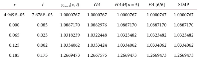
Using GA by the same procedure as in example 1, we get the optimal solution is found after 51 generation to converge to the exact solution, where x = 4.9489E−05 and t=7.6780E−05. After execute the Equation (43) many times
by using GA as in Table 2 we found the optimal solution.
4.2. Singular Wave-Type Equations
Example 3. Now, we consider the inhomogeneous singular wave-type equation,
(
2)
3 52
5 4 12 5 4 ,
xx x tt
y y x y y x x x
x
+ − + = + − − (45)
[image:10.595.207.542.628.729.2]subject to initial conditions
Table 2. Optimal solution of genetic algorithm for example 2.
x t yExact(x, t) GA HAM(n = 5) PA [6/6] SIMP
( )
0, e ,t( )
0, 0.x
y t = − y t = (46)
To solve Equations (45)-(46) by means of the standard HAM, we choose the initial approximation
( )
0 , e ,
t
y x t = − (47)
and the linear operator
(
)
2(
2)
(
)
, ; 2 , ;
, ; x t q x t q ,
L x t q
x x
x
φ φ
φ =∂ + ∂
∂ ∂ (48)
with the property
1
2 0,
c
L c
x
− + =
(49)
where ci
(
i=1, 2)
are constants of integration. Furthermore, Equation (45)suggests that we define the nonlinear operator as
(
)
(
)
(
)
(
)
(
)
(
)
(
)
2
2 2
2
3 2
, ; 2 , ;
, ; 5 4 , ;
, ;
12 5 4 .
x t q x t q
N x t q x x t q
x x
x
x t q
x x x
t
φ φ
φ φ
φ
∂ ∂
= + − +
∂ ∂
∂
− − − −
∂
Using the above definition, we construct the zeroth-order deformation equa-tion as in (7) and (8) and the mth-order deformation equation for m≥1 is
( )
, 1( )
,(
1)
,m m m m m
L y x t −χ y − x t =hR y − (50)
with the initial conditions
( )
0, 0,( ) ( )
0, 0m m x
y t = y t = (51)
where
(
) (
)
(
)
(
)
(
) (
)
(
)
2
1 1 1 1
3 4
1
2
5 4
1 12 5 4 .
m m m xx m x m
m tt m
R y y x y
x
y χ x x x
− − − −
−
= + − +
− − − − −
y
(52)
Now, the solution of the mth-order deformation Equation (50) for m≥1 is
( )
( )
2 2(
)
1 0 0 1
, , x x .
m m m m m
y x t =χ y − x t +h x
∫ ∫
− x R y − (53)We now successively obtain
( )
( )
(
)
4 2 7 5 3
1
2 8 2 6 2 4 4 2 2 2 2 11
2
2 9 2 7 2 5 2 3
1 1 1
, e ,
5 14 6
1 13 1 1 1
, e
90 105 10 5 462
43 43 1 1 1
,
3780 336 14 3 6
t
t
y x t x x h x x x h
y x t h x h x h x hx h x hx h x
h x h h x h h x h h x
−
−
= − + + + −
= + + − − − −
− + + + + − +
(54)
( )
0( )
( )
1, , m , ,
m
y x t y x t y x t
+∞
=
= +
∑
(55)Hence, the series solution when h= −1 is given by
( )
3 2 1 4 1 6 1 8, 1 e noise terms.
2! 3! 4!
t
y x t =x + + x + x + x + x + − +
(56)
This series has the closed form as n→ ∞
( )
3 2, ex t,
y x t =x + − (57)
which is the exact solution of the problem (45)-(46) compatible with ADM [8]. Notice that the noise terms that appear between various components vanish in the limit.
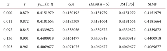
Using GA by the same procedure as in example 1, we get the optimal solution is found after 51 generation to converge to the exact solution, where x=0 and
0.879
t= . After execute the Equation (56) many times by using GA as in Table 3
we found the optimal solution
Example 4. We now examine the inhomogeneous wave-type equation,
(
4)
(
4)
24
18 9 2 18 9 ,
xx x tt
y y x x y y x x t
x
+ − + = − − + (58)
subject to initial conditions
( )
2( )
0, 1 , x 0, 0.
y t = +t y t = (59)
To solve Equations (58)-(59) by means of the standard HAM, we choose the initial approximation
( )
20 , 1 ,
y x t = +t (60)
and the linear operator
(
)
2(
2)
(
)
, ; 4 , ;
, ; x t q x t q ,
L x t q
x x
x
φ φ
φ =∂ + ∂
∂ ∂ (61)
with the property
1
2 0,
3
c
L c
x
− + =
(62)
where ci
(
i=1, 2)
are constants of integration. Furthermore, Equation (58) [image:12.595.208.542.627.729.2]suggests that we define the nonlinear operator as
Table 3. Optimal solution of genetic algorithm for example 3.
x t yExact(x, t) GA HAM(n = 5) PA [5/5] SIMP
(
)
(
)
(
)
(
)
(
)
(
)
(
)
2
4 2
2
4 2
2
, ; 4 , ;
, ; 18 9 , ;
, ;
18 9 2.
x t q x t q
N x t q x x x t q
x x
x
x t q
x x t t
φ φ
φ φ
φ
∂ ∂
= + − +
∂ ∂
∂
− + + +
∂
(63)
Using the above definition, we construct the zeroth-order deformation equa-tion as in (7) and (8) and the mth-order deformation equation for m≥1 is
( )
, 1( )
,(
1)
,m m m m m
L y x t −χ y − x t =hR y − (64)
with the initial conditions
( )
0, 0,( )
( )
0, 0m m x
y t = y t = (65)
where
(
) (
)
(
)
(
)
(
) (
)
(
)
4
1 1 1 1
4 2
1
4
18 9
1 18 9 2 .
m m m xx m x m
m tt m
R y y x x y
x
y χ x x t
− − − −
−
= + − +
− + − + +
y
(66)
Now, the solution of the mth-order deformation Equation (64) for m≥1 is
( )
( )
4 4(
)
1 0 0 1
, , x x .
m m m m m
y x t =χ y − x t +h x
∫ ∫
− x R y − (67)We now successively obtain
( )
( )
(
) (
)
( )
(
) (
)
6 3
1
2 12 2 9 2 6 2 3
2
3 18 3 15 3 2 12 3 2 9
3
3 2 6 3 2 3
1
, ,
6
1 1 1
, ,
120 9 6
1 23 1 1 1 2
,
5040 5400 90 60 6 9
1
3 2 2 ,
6
y x t hx hx
y x t h x h x h h x h h x
y x t h x h x h h x h h x
h h h x h h h x
= − −
= + + − − +
= − − − − + +
+ + − − + +
(68)
and so on, in this manner the rest of the iterations can be obtained. Thus, the approximate solution in a series form is given by
( )
0( )
( )
1
, , m , ,
m
y x t y x t y x t
+∞
=
= +
∑
(69)Thus, the series solution when h= −1 is given by
( )
, 2 1 3 1 6 1 9 1 12 .2! 3! 4!
y x t = + +t x + x + x + x +
(70)
This series has the closed form as n→ ∞
( )
2 3, e ,x
y x t = +t (71)
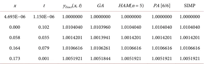
which is the exact solution of the problem (58)-(59) compatible with ADM [8]. Using GA by the same procedure as in example 1, we get the optimal solution is found after 51 generation to converge to the exact solution, where x = 4.6903E−06 and t=1.1498E−06. After execute the Equation (70) many times
Table 4. Optimal solution of genetic algorithm for example 4.
x t yExact(x, t) GA HAM(n = 5) PA [6/6] SIMP
4.693E−06 1.150E−06 1.0000000 1.0000000 1.0000000 1.0000000 1.0000000 0.000 0.102 1.0104040 1.0103960 1.0104040 1.0104040 1.0104040 0.058 0.035 1.0014201 1.0013941 1.0014201 1.0014201 1.0014201 0.164 0.079 1.0106616 1.0106261 1.0106616 1.0106616 1.0106616 0.173 0.001 1.0051921 1.0051844 1.0051921 1.0051921 1.0051921
4.3. Nonlinear Models
In what follows we close this analysis by examining two nonlinear time-de- pendent equations
Example 5. We now consider the nonlinear time-dependent equation,
(
2 2)
2 25
24 16 e 2 e ,
y y
xx x t
y y t t x x y
x
+ + + − = (72)
subject to initial conditions
( )
0, 0, x( )
0, 0.y t = y t = (73)
To solve Equations (72)-(73) by means of the standard HAM, we choose the initial approximation
( )
0 , 0,
y x t = (74)
and the linear operator
(
)
2(
2)
(
)
, ; 5 , ;
, ; x t q x t q ,
L x t q
x x
x
φ φ
φ =∂ + ∂
∂ ∂ (75)
with the property
1
2 0,
4
c
L c
x
− + =
(76)
where ci
(
i=1, 2)
are constants of integration. Furthermore, Equation (72)suggests that we define the nonlinear operator as
(
)
(
)
(
)
(
)
( )( )
(
)
2
, ;
2 2
2
, ;
2 2
, ; 5 , ;
, ; 24 16 e
, ;
2 e .
x t q
x t q
x t q x t q
N x t q t t x
x x
x
x t q x
t
φ
φ
φ φ
φ
φ
∂ ∂
= + + +
∂ ∂
∂
− −
∂
(77)
Using the above definition, we construct the zeroth-order deformation equa-tion as in (7) and (8) and the mth-order deformation equation for m≥1 is
( )
, 1( )
,(
1)
,m m m m m
L y x t −χ y − x t =hR y − (78)
with the initial conditions
( )
0, 0,( )
( )
0, 0m m x
y t = y t = (79)
(
) (
)
(
)
(
2 2)
2(
)
1 1 1 1 1 1
5
24 16 2 .
m m m xx m x m m m t
R y y t t x A x B y
x
− = − + − + + − − − − −
y (80)
For the nonlinear terms ( , ; )
1 1
e x t q m
m
A
φ ∞
− =
=
∑
and ( , ;2 )1 1
e
x t q
m m B φ ∞ − =
=
∑
, thecorres-ponding Adomian polynomials [15][16] are:
0 0 0 0 0 0 1 1 2
2 2 1
3
3 3 1 2 1
2 2 4
4 4 2 1 3 1 2 1
e , e , 1 e , 2! 1 e , 3!
1 1 1
e ,
2! 2! 4!
y y y y y A A y
A y y
A y y y y
A y y y y y y y
= = = + = + + = + + + + (81) and 0 0 0 0 0 2 0 2 1 1 2 2
2 2 1
2 3
3 3 1 2 1
2
2 2 4
4 4 2 1 3 1 2 1
e ,
1 e , 2
1 1 1
e , 2 4 2!
1 1 1 1
e ,
2 4 8 3!
1 1 1 1 1 1 1 1
e ,
2 4 2! 4 8 2! 16 4!
y y y y y B B y
B y y
B y y y y
B y y y y y y y
= = = + = + + = + + + + (82)
Now, the solution of the mth-order deformation Equation (78) for m≥1 is
( )
( )
5 5(
)
1 0 0 1
, , x x .
m m m m m
y x t =χ y − x t +h x
∫ ∫
− x R y − (83)We now successively obtain
( )
( )
(
)
2 4 4 2
1
2 4 2 2 2 8 2 3 2 6
2
2 2 2 2 4 2 2
1 1
, 2 ,
2 16
1 1 1 11 3
,
12 64 1536 15 40
1 1 1
2 2 ,
2 8 16
y x t ht x hx htx
y x t h t h t h x h t h t x
h t ht h h x h h tx
= − + = − + + − + + − − + + (84)
and so on, in this manner the rest of the iterations can be obtained. Thus, the approximate solution in a series form is given by
( )
0( )
( )
1
, , m , ,
m
y x t y x t y x t
+∞
=
= +
∑
(84)( )
, 2 2 1 2 4 1 3 6 1 4 8 noise terms.2 3 4
y x t = − tx − t x + t x − t x + +
(85)
This series has the closed form as n→ ∞
( )
(
2)
, 2 ln 1 ,
y x t = − +tx (86)
which is the exact solution of the problem (72)-(73) compatible with ADM [8]. Notice that the noise terms that appear between various components vanish in the limit.
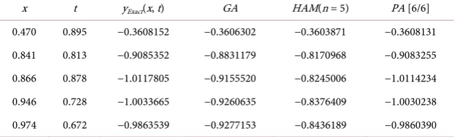
Using GA by the same procedure as in example 1, we get the optimal solution is found after 51 generation to converge to the exact solution, where x=0.470
[image:16.595.234.537.71.137.2] [image:16.595.208.542.629.729.2]and t=0.895. After execute the Equation (85) many times by using GA as in
Table 5 we found the optimal solution
Example 6. Finally, we examine the nonlinear homogeneous equation,
(
4)
6
14 4 ln ,
xx x tt
y y t x y ty y y
x
+ + + + = (87)
subject to initial conditions
( )
0, 1, x( )
0, 0.y t = y t = (88)
To solve Equations (87)-(88) by means of the standard HAM, we choose the initial approximation
( )
0 , 1,
y x t = (89)
and the linear operator
(
)
2(
2)
(
)
, ; 6 , ;
, ; x t q x t q ,
L x t q
x x
x
φ φ
φ =∂ + ∂
∂ ∂ (90)
with the property
1
2 0,
5
c
L c
x
− + =
(91)
where ci
(
i=1, 2)
are constants of integration. Furthermore, Equation (87)suggests that we define the nonlinear operator as
(
)
(
)
(
)
(
)
(
)
(
)
(
)
(
)
2
4 2
2
2
, ; 6 , ;
, ; 14 , ;
, ;
4 , ; ln , ; .
x t q x t q
N x t q t x x t q
x x
x
x t q t x t q x t q
t
φ φ
φ φ
φ
φ φ
∂ ∂
= + + +
∂ ∂
∂
+ −
∂
(92)
Table 5. Optimal solution of genetic algorithm for example 5.
x t yExact(x, t) GA HAM(n = 5) PA [6/6]
Using the above definition, we construct the zeroth-order deformation equa-tion as in (7) and (8) and the mth-order deformation equation for m≥1 is
( )
, 1( )
,(
1)
,m m m m m
L y x t −χ y − x t =hR y − (93)
with the initial conditions
( )
0, 0,( )
( )
0, 0m m x
y t = y t = (94)
where
(
) (
)
(
)
(
4)
(
)
1 1 1 1 1 1
6
14 4 .
m m m xx m x m m m tt
R y y t x y tA y
x
− = − + − + + − + − − −
y (95)
For the nonlinear term
(
)
(
)
11
, ; ln , ; m
m
x t q x t q A
φ φ ∞ −
=
=
∑
, the correspondingAdomian polynomials [15][16] are:
(
)
(
)
(
)
(
)
0 0 0
1 0 1
2
2 0 2 1
0
3
3 0 3 1 2 2 1
0 0
2 2 4
4 0 4 2 1 3 2 1 2 3 1
0 0 0
ln ,
1 ln ,
1 1
1 ln ,
2!
1 1 1
1 ln ,
3!
1 1 1 1 2 1
1 ln ,
2! 2! 4!
A y y
A y y
A y y y
y
A y y y y y
y y
A y y y y y y y y
y y y
= = + = + + = + + − = + + + − + (96)
Now, the solution of the mth-order deformation Equation (93) for m≥1 is
( )
( )
6 6(
)
1 0 0 1
, , x x .
m m m m m
y x t =χ y − x t +h x
∫ ∫
− x R y − (97)We now successively obtain
( )
( )
(
)
(
)
( )
(
)
(
)
(
)
(
)
(
)
6 2 12 12 2 8 2 6 2 2 4 2 2
2
3 18 3 14 3 2 12
3
3 2 10 3 2 8 3 3 2 6
3 2 2 4 3 2 2
1
, ,
66
1 7 1 1
, ,
13464 572 66 2
1 965 1
,
5574096 18290844 6732
67 7 1
11 2
12870 286 66
2 ,
y x t hx htx
y x t h x h tx h h x h t x h h tx
y x t h x h tx h h x
h t x h h tx h t h h x
h h t x h h h tx
= + = + + + + + + = + + + + + + + + + + + + + + (98)
and so on, in this manner the rest of the iterations can be obtained. Thus, the approximate solution in a series form is given by
( )
0( )
( )
1
, , m , ,
m
y x t y x t y x t
+∞
=
= +
∑
(99)Thus, the series solution when h= −1 is given by
( )
2 1 2 4 1 3 6 1 4 8, 1 .
2! 3! 4!
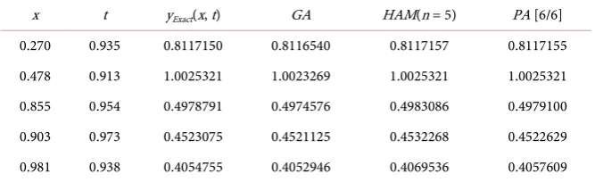
Table 6. Optimal solution of genetic algorithm for example 6.
x t yExact(x, t) GA HAM(n = 5) PA [6/6]
0.270 0.935 0.8117150 0.8116540 0.8117157 0.8117155
0.478 0.913 1.0025321 1.0023269 1.0025321 1.0025321
0.855 0.954 0.4978791 0.4974576 0.4983086 0.4979100
0.903 0.973 0.4523075 0.4521125 0.4532268 0.4522629
0.981 0.938 0.4054755 0.4052946 0.4069536 0.4057609
This series has the closed form as n→ ∞
( )
2, etx ,
y x t = − (101)
which is the exact solution of the problem (87)-(88) compatible with ADM [8]. Using GA by the same procedure as in example 1, we get the optimal solution is found after 51 generation to converge to the exact solution, where x=0.270
and t=0.935. After execute the Equation (100) many times by using GA as in
Table 6 we found the optimal solution.
5. Conclusions
To our best knowledge, this is the first result on the application of the HAM with GA to solve models of the time-dependent Emden-Fowler type of equations and wave-type equation with singular behaviors. The HAM with GA has been suc-cessfully applied to solve models of the time-dependent Emden-Fowler type of equations and wave-type equation with singular behaviors. The HAM with GA has worked effectively to handle these models giving it a wider applicability. The proposed scheme of HAM has been applied directly without any need for trans-formation formulae or restrictive assumptions. The solution process of HAM is compatible with those methods in the literature providing analytical approxima-tion such as ADM.
The approach of HAM with GA has been tested by employing the method to obtain approximate-exact solutions of six examples. The results obtained in all cases demonstrate the reliability and the efficiency of this method.
Acknowledgements
We would like to thank the referees for their careful review of our manuscript.
References
[1] Davis, H.T. (1962) Introduction to Nonlinear Differential and Integral Equations. Dover Publications, New York.
[2] Chandrasekhar, S. (1967) Introduction to the Study of Stellar Structure. Dover Pub-lications, New York.
[3] Richardson, O.U. (1921) The Emission of Electricity from Hot Bodies. London. [4] Adomian, G., Rach, R. and Shawagfeh, N.T. (1995) On the Analytic Solution of
https://doi.org/10.1007/BF02187585
[5] Shawagfeh, N.T. (1993) Nonperturbative Approximate Solution for Lane-Emden Equation. Journal of Mathematical Physics, 34, 4364-4369.
https://doi.org/10.1063/1.530005
[6] Wazwaz, A.M. (2001) A New Method for Solving Differential Equations of the Lane-Emden Type. Applied Mathematics and Computation,118, 287-310.
[7] Wazwaz, A.M. (2005) Adomian Decomposition Method for a Reliable Treatment of the Emden-Fowler Equation. Applied Mathematics and Computation, 161, 543-560. [8] Wazwaz, A.M. (2005) Analytical Solution for the Time-Dependent Emden-Fowler Type of Equations by Adomian Decomposition Method. Applied Mathematics and Computation, 166, 638-651.
[9] Yıldırım, A. and Öziş, T. (2009) Solutions of Singular IVPs of Lane-Emden Type by the Variational Iteration Method. Nonlinear Analysis, 70, 2480-2484.
[10] Dehghan, M. and Shakeri, F. (2008) Approximate Solution of a Differential Equa-tion Arising in Astrophysics Using the VariaEqua-tional IteraEqua-tion Method. New Astron-omy, 13, 53-59.
[11] Liao, S.J. (2003) Beyond Perturbation: Introduction to the Homotopy Analysis Me-thod. Chapman and Hall, CRC Press, Boca Raton.
https://doi.org/10.1201/9780203491164
[12] He, J.H. (2003) Homotopy Perturbation Method: A New Nonlinear Analytical Technique. Applied Mathematics and Computation, 135, 73-79.
[13] Gen, M. and Cheng, R. (1997) Genetic Algorithms and Engineering Design. John Wiley & Sons, Hoboken.
[14] Melanie, M. (1998) An Introduction to Genetic Algorithms. MIT Press, Cambridge. [15] Adomian, G. (1989) Nonlinear Stochastic Systems Theory and Applications to
Physics. Kluwer Academic Publishers, Dordrecht. https://doi.org/10.1007/978-94-009-2569-4
[16] Wazwaz, A.M. (2000) A New Algorithm for Calculating Adomian Polynomials for Nonlinear Operators. Applied Mathematics and Computation, 111, 53-69.
Submit or recommend next manuscript to SCIRP and we will provide best service for you:
Accepting pre-submission inquiries through Email, Facebook, LinkedIn, Twitter, etc. A wide selection of journals (inclusive of 9 subjects, more than 200 journals)
Providing 24-hour high-quality service User-friendly online submission system Fair and swift peer-review system
Efficient typesetting and proofreading procedure
Display of the result of downloads and visits, as well as the number of cited articles Maximum dissemination of your research work
Submit your manuscript at: http://papersubmission.scirp.org/