Mesh free methods for liquid crystal simulation

YAKUTOVICH, Mikhail.

Available from Sheffield Hallam University Research Archive (SHURA) at:

http://shura.shu.ac.uk/20580/

This document is the author deposited version. You are advised to consult the publisher's version if you wish to cite from it.

Published version

YAKUTOVICH, Mikhail. (2009). Mesh-free methods for liquid crystal simulation. Doctoral, Sheffield Hallam University (United Kingdom)..

Copyright and re-use policy

See http://shura.shu.ac.uk/information.html

Sheffield Hallam University Research Archive

I- Sheffield s i 1W8

1 0 1 923 0 4 7 9

Z b d h

I Sheffield Hailam University I Learning and IT Services

j Adsetts Centre City Campus

* S ftgjteid S t 1WB

All rights reserved

INFORMATION TO ALL USERS

The quality of this reproduction is dependent upon the quality of the copy submitted.

In the unlikely event that the author did not send a com plete manuscript and there are missing pages, these will be noted. Also, if material had to be removed,

a note will indicate the deletion.

uest

ProQuest 10701227

Published by ProQuest LLC(2017). Copyright of the Dissertation is held by the Author.

All rights reserved.

This work is protected against unauthorized copying under Title 17, United States C ode Microform Edition © ProQuest LLC.

ProQuest LLC.

789 East Eisenhower Parkway P.O. Box 1346

Mesh-Free M ethods

for Liquid Crystal Simulation

Mikhail Yakutovich

A thesis submitted in partial fulfilment of the requirements of

Sheffield Hallam University

for the degree of Doctor of Philosophy

Abstract

The key aim of this Thesis is the development and implementation of a set of sim­ ulation techniques for LCs capable of tackling mesoscopic phenomena. In this, we concentrate only on mesh-free particle numerical techniques. Two broad approaches are used, namely bottom-up and top-down.

While adopting the bottom-up approach, we employ the DPD method as a foun­ dation for devising a novel LC simulation technique. In this, we associate a traceless symmetric order tensor, Q, with each DPD particle. We then further extend the DPD forces to directly incorporate the Q tensor description so as to recover a more complete representation of LC behaviour. The devised model is verified against a number of qualitative examples and applied to the simulation of colloidal particles immersed in a nematic LC. We also discuss advantages of the developed model for simulation of dynamic mesoscopic LC phenomena.

In the top-down approach, we utilise recently emergent numerical mesh-free methods. Specifically, we use the SPH method and its variants. The developed method includes hydrodynamics, variable order parameter and external electric and magnetic fields. The developed technique is validated against a number of analytical and numerical solutions.

M oum podumejisiM noce^iu^aemcsi1

Acknowledgements

First of all I would like to express my sincere gratitude to my supervisors, Dr D.J. Cleaver and Prof C.M. Care, for their constant support and guidance throughout this project. All the time they provided me with clear explanations, important advice and lots of good ideas, without which I would have been lost. I would also like to thank Dr I. Halliday, Dr T.J. Spencer, Dr C.J.P. Newton and colleagues from Hewlett-Packard for their useful comments and advice.

I am grateful to David, Christina, Anna and Sergey who, from the very beginning, helped me to acclimatise in Sheffield and then made it such a great place to study. Many thanks to all colleagues from Sheffield Hallam University with whom I spent last three years or so. So thanks to Laurence, Fatima, Candy, Adam, Stephen, Vin, Alena, Alex and Pavel. I would also like to thank an endless stream of my friends who made Sheffield such an enjoyable place to stay. So thank you to Will, Lee, Olesya, Sasha, Juri, Dima, Sveta, Viktor and Iryna Yarmolenko, Masha, Maksim, Antonia, Paul, Taras, Gena, Artem, Viktor Nikitin, Nastya Sheiko, Nastya Dontsova, Irchik and many others.

Advanced Studies

The following is a chronological list of related postgraduate work undertaken and meetings attended during the course of study:

• “DL POLY Training Day”, Sheffield University (April 2006).

• “Applied Numerical Algorithms” course, Edinburgh Parallel Computing Cen­ tre (June 2006).

• CCP5 Summer School 2006 “Methods in Molecular Simulation”, Cardiff Uni­ versity (July 2006).

• Graduate Training Assistant Workshops, Sheffield Hallam University (Novem­ ber 2006 - February 2007).

• MERI Research Methods module, Sheffield Hallam University (February 2007).

• Advanced Measurement Techniques training module, MERI, Sheffield Hallam University (March 2007).

• “Mainz Materials Simulation Days”, Mainz, Germany (June 2007). Poster presentation “Smoothed dissipative particle nemato dynamics: from atomistic to application scale”.

• MERI 2nd Year Student Seminar Day, Sheffield Hallam Univeristy (20th June 2007). Oral presentation “Mesh free simulation of liquid crystals using modi­ fied smoothed particle hydrodynamics”

• 9th European Conference on Liquid Crystals, Lisbon, Portugal (July 2007). Poster presentation “Smoothed dissipative particle nemato dynamics: from atomistic to application scale”.

• CCP5 Annual General Meeting 2007 “Multiscale Modelling: simulation meth­ ods and applications spanning time and length scales”, Cambridge. Poster

presentation “Smoothed dissipative particle nemato dynamics: from atomistic to application scale”.

• Computer Modelling Seminar at Sheffield University (November 2007). In­ vited talk “Smoothed dissipative particle nemato dynamics: from continuum to mesoscale”.

• ‘Liquid Crystal Micro- and Nano-Composites”’ meeting, Manchester (9th Jan­ uary 2008). Poster presentation “Smoothed dissipative particle nemato dy­ namics: from atomistic to application scale”.

• “Bistable displays: technologies & application” conference, Hewlett Packard Laboratories, Bristol (25th June 2008).

• “Dissipative Particle Dynamics” CECAM workshop, Lausanne, Switzerland (July 2008). Poster presentation “Smoothed dissipative particle nemato dy­ namics: from atomistic to application scale”.

• “Liquid Crystals for Photonics” workshop, Cambrdige (July 2008). Oral pre­ sentation “Mesh free simulation of liquid crystals using modified smoothed particle hydrodynamics”.

• 23rd BLCS Conference 2009, Hewlett Packard Laboratories, Bristol (April 2009). Oral presentation “Studying bistability in liquid crystal devices with complex 3-D topologies using mesh-free methods”.

Publications

This thesis contains some work published in the following journals:

• M. V. Yakutovich, C. J. P. Newton, and D. J. Cleaver. Mesh-Free Simulation of Complex LCD Geometries. Molecular Crystals and Liquid Crystals, 502:1, 245-257, 2009.

Contents

List of Acronyms xi

1 Introduction 1

1.1 Aims & O b jectiv es... 2

1.2 Thesis Structure... 2

1.3 Liquid C ry s ta ls ... 3

1.3.1 The Fundamentals of Liquid C ry stals... 3

1.3.2 Physical Properties of Liquid Crystals ... 6

1.3.3 Computer Simulation of Liquid C ry s ta ls ... 8

1.3.4 Liquid Crystal Displays ... 11

1.4 B istability... 13

1.4.1 Zenithal Bistable Device (Z B D )... 14

1.4.2 Post Aligned Bistable Nematic (PABN)...15

1.5 Basics of Mesh-free M ethods... 15

1.5.1 Mesh-free Particle M e th o d s ... 16

1.5 .2 Consistency, Completeness and Reproducing Conditions . . . 16

2 Landau-de Gennes Theory of Liquid Crystals 19 2.1 Introduction... 19

2.1.1 The Nematic Order Param eter... 19

2.1 .2 The Biaxiality... 20

2.1.3 The Tensor Order Parameter Q ... 22

2.1.4 The Nematic-Isotropic Phase T ra n s itio n ...23

2 .2 Static Theory of Liquid C rystals...26

2.2.1 E la s tic ity ...26

2.2.2 Electric and Magnetic F ields...27

2.2.3 Flexoelectricity... 29

2.2.4 Boundary Conditions and A nchoring...30

2.2.5 The Equilibrium S tates... 31

2.2.6 Defects...33

2.3 Dynamic Theory of Liquid C ry stals...34

2.3.1 Dynamic E quations...37

3 M esoscopic M esh-free Particle Techniques 39 3.1 Introduction...39

3.2 Dissipative Particle D ynam ics... 40

3.2.1 DPD Formalism... 41

3.2.2 Equilibrium P ro p erties... 43

3.2.3 Hydrodynam ics... 45

3.2.4 Fluid Particle M o d e l...50

3.2.5 DPD D raw b ack s... 53

3.3 Smoothed Particle H ydrodynam ics...55

3.3.1 SPH Form alism ... 55

3.3.2 SPH Conservation Law E quations... 59

3.3.3 SPH Artificial V isc o sity ... 60

3.3.4 Completeness of the SPH ... 62

3.3.5 SPH Drawbacks and Im provem ents...64

3.3.6 Corrective Smoothed Particle M ethod...67

3.3.7 Modified Smoothed Particle H ydrodynam ics...6 8 3.4 Smoothed Dissipative Particle D ynam ics... 70

3.5 Other Mesoscopic Mesh-free Particle Techniques... 72

3.5.1 Direct Simulation Monte Carlo ...72

3.5.2 Stochastic Rotational D ynam ics...74

4 Im plem entation of Bottom -up Approaches 76 4.1 Practical Aspects in DPD/FPM Implementation... 76

4.1.1 Reduced Units ... 77

4.1.2 Periodic Boundary Conditions / Minimum Image Convention . 78 4.1.3 Integrators... 79

4.1.4 Q uaternions...80

4.1.5 Verlet Neighbour L ist...82

4.1.6 Calculation of Observables... 83

4.2 DPD/FPM Testing and Verification...85

4.3 Extending DPD for the Simulation of Liquid C ry stals...90

4.3.1 Incorporation of a Q-tensor into DPD F o rm a lism ... 92

4.3.2 Extending Conservative Forces...93

CONTENTS ix

4.3.4 Extending the Thermostat F o rces... 96

4.4 Simulation R e s u lts ...98

4.4.1 Recovering the Isotropic-Nematic Phase T ra n s itio n ...98

4.4.2 Diffusion Coefficients...98

4.4.3 Simulation of Colloidal Particles Immersed in L C s ... 99

4.5 Discussion... 101

4.6 Conclusions and Future W o r k ...103

5 Im plem entation of Top-down Approaches 104 5.1 Revising the Governing Equations ...104

5 .2 Description of the Algorithm ...106

5.3 Major Practical Implementation A sp e c ts... 108

5.3.1 Boundary C onditions...108

5.3.2 Time Integration Scheme... 109

5.3.3 Smoothing L e n g th ... 110

5.3.4 Smoothing K ernel... I l l 5.3.5 Reduced Units ...112

5.4 Implementation Details For Individual M e th o d s... 112

5.4.1 Smoothed Particle H ydrodynam ics... 112

5.4.2 Modified Smoothed Particle H ydrodynam ics...113

5.5 Electric Field S olvers...114

5.6 SPH Simulation A tte m p ts ... 117

5.7 MSPH Testing and V erification... 121

5.7.1 Equilibrium Phase B eh a v io u r...121

5.7.2 Freedericksz T ransition...122

5.7.3 Transverse Flow E ffe c t...124

5.7.4 Fast Switching Dual-Frequency Chiral HAN C ell...126

5.8 C onclusions...129

6 M odelling of the PA BN D evice 130 6.1 Overview of PABN O p eratio n ...130

6.1.1 Experimental S tudies...130

6.1.2 Theoretical and Simulation S tu d ie s... 132

6.2 Post Geometry Representation...133

6.2.1 Geometry M o d e l... 133

6.2.2 Geometry D iscretisation... 135

6.2.3 Implementation D etails...139

6.3.1 Tilted State

T

... 142

6.3.2 Planar State V \... 142

6.4 Studying Effects of the Post T opography...145

6.4.1 Circular P o sts ...145

6.4.2 Effect of the Post Sm oothness... 146

6.4.3 Effect of the Post H eig h t...148

6.5 Switching B eh a v io u r...150

6.5.1 T - V T ran sitio n ... 151

6.5.2 V - T T ran sitio n ... 153

6 .6 C onclusions...153

7 Conclusions and Further Work 156 7.1 Conclusions and Discussions...156

7.2 Further W o r k ...158

A M oving Least Squares Shape Functions 160

List of Acronyms

C SPM Corrective smoothed particle method D P D Dissipative particle dynamics

D SM C Direct simulation Monte Carlo E L P Ericksen-Leslie-Parodi theory FD M Finite-difference method F E M Finite-elements method F P E Fokker-Planck equation F P M Fluid particle model

G C M C Grand Canonical Monte Carlo H A N Hybrid-aligned nematic

LB Lattice Boltzmann

LC Liquid crystal

LCD Liquid crystal display

LJ Lennard-Jones

M C Monte Carlo

M D Molecular dynamics

M SP H Modified smoothed particle hydrodynamics PA B N Post-aligned bistable nematic

Chapter 1

Introduction

Liquid crystals (LC) are fascinating materials which combine the usual properties of conventional fluids with an inherent orientational ordering. This leads to LCs exhibiting a range of anisotropic properties, which give them a marked technological significance. LCs have found applications in many areas of physical and biological science and engineering, such as in liquid crystal displays (LCDs), optoelectronic devices, sensors, commercial detergents (soap), biological self-assembly of micelles etc.

Some aspects of LC behaviour have been well-studied since they were first dis­ covered in 1890. In theoretical studies, computer modelling plays an important part in aiding understanding of many processes on atomistic and mesoscopic levels. It also certainly helps with explaining and predicting behaviour of LC devices on continuum length-scales. For example, the multi-billion pound LCD industry has motivated the development of LC solvers based on Ericksen-Leslie-Parodi contin­ uum theory. However, there are still some important gaps in our understanding of the physics behind LCs. This is due, in part, to the to complex interplay of distinct physical phenomena on different time- and length-scales in these systems, e.g. inter-molecule interactions, orientational order, continuum velocity field etc are all coupled. This makes it impossible to fully study LCs with only one chosen simulation technique.

Thus, nowadays the predominant issue in the computer modelling of materials and, particulary, of LCs, is the problem of bridging the length- and time-scales between the underlying molecular motions and the consequent application-scale be­ haviour. A wide range of techniques have been developed to address this amongst which may be included accelerated molecular dynamics (MD) methods, Brownian dynamics, dissipative particle dynamics (DPD), Lattice Boltzmann (LB), smoothed particle hydrodynamics (SPH) and a suite of methods which combine elements of

CHAPTER 1. INTRODUCTION 2

these approaches. While it is unlikely that a single unified framework will be emer­ gent from this multiplicity of developments, a common approach is to develop “over­ lap” methods which allow a particular coarse grained method to be paramaterised using a finer grained method. Given this broad context, the work presented in this Thesis can be viewed as an attempt to identify and fill gaps in the current spectrum of LC modelling approaches.

1.1 Aims & Objectives

This Thesis mainly deals with the development of novel mesoscopic simulation tech­ niques for simulating LCs. This direction was primarily determined at the start of this project, when the following objectives were set:

• to determine which mesoscopic simulation techniques can be applied to simu­ lation of LCs, both from bottom-up and top-down points of view, in order to bridge the gaps between existing simulation methodologies.

• to consider bottom-up approach simulation techniques and to determine if a comprehensive link with the atomistic level can be established.

• to consider top-down simulation techniques and to investigate how thermal noise can be incorporated into the model, so as to properly recover the meso­ scopic behaviour.

• to determine how these models compare to conventional numerical techniques in terms of computational requirements.

• to investigate if the developed simulation techniques are computationally vi­ able and whether they can address LC phenomena which are non-achievable with the currently available simulation techniques.

1.2 Thesis Structure

The remainder of this Chapter is devoted to a brief introduction to LCs and LCDs. This is followed by a precis of the basics of mesh-free simulation methods.

In Chapter 3 we give an overview of mesoscopic simulations using mesh-free particle techniques. We place a particular emphasis on dissipative particle dynamics (DPD) and smoothed particle hydrodynamics (SPH), the relevant specifics of which are considered in more detail.

In Chapter 4 we describe a novel LC simulation technique based on a bottom- up DPD approach. We first show how this novel approach can be tuned to yield anisotropic static and dynamic behaviour of LCs. We then apply this method to the demanding scenario of 3-D simulation of dynamic behaviour of colloidal particles immersed in a nematic LC.

In Chapter 5 we follow a top-down approach, in which we apply the modified smoothed particle hydrodynamics (MSPH) mesh-free numerical technique to the simulation of LCs. We first describe our unsuccessful attempts to model LCs with a number of simpler techniques, such as with SPH, corrective smoothed particle method (CSPM) and some of their variants. Then, we provide results obtained using our MSPH approach for a number of test cases so as to address the validity of the newly developed solver.

In Chapter 6 we present a study performed using our mesh-free simulation ap­ proach to investigate the statics and dynamics of the post-aligned bistable nematic (PABN) device. Here, we briefly describe the PABN device, our model geometry representation and the approach we use to discretise it. We then provide results obtained on static configurations for a number of different post geometries. Finally, we provide some results on the PABN device switching behaviour.

In Chapter 7 we conclude with a summary of this Thesis and suggest some ideas for future work. A bibliography is included.

1.3 Liquid Crystals

In this section we give a short introduction to the physics of liquid crystals (LCs), provide a brief overview of the available LC simulation techniques and describe the most common application of LCs in liquid crystal displays (LCDs).

1.3.1 The Fundamentals of Liquid Crystals

CHAPTER 1. INTRODUCTION 4

matter possesses some fluidity, and crystal, which indicates the presence of long- range order in the system. In the crystalline solid state, the order is both positional and orientational, i.e. molecules occupy specific positions and their molecular axes are pointed in a certain direction. In a liquid phase, in contrast, there is no long- range order and the matter is fully isotropic. Molecules in LC phases, however, have orientational order and either no or only partial positional order. In almost all cases, these phases are only formed when molecules are anisotropic in shape - usually they are rod-like or disk-like. Most LC materials are organic compounds, and the classical example is p-azoxyanisole (PAA) shown in Fig. 1.1. From a steric point of view, this molecule is a rigid rod of length ~ 20 A and width 5 A [1].

O — CH,

■N=N-O

Figure 1.1: Formula of p-azoxyanisole.

LC phases are often called mesophases (from mesomorphic - of intermediate form), and, from the same root, their constituent molecules are called mesogens.

This is a well-established nomenclature nowadays.

LCs can be divided in two classes, namely thermotropic and lyotropic. Ther­ motropic LCs are formed by mesogens in a certain range of temperatures Tm <

T < Tin, where Tm is the melting temperature of the crystalline phase and Tin is the temperature of isotropic-nematic LC phase transition. The properties of ther­ motropic LCs are very dependant on temperature, and that is why they have thermo-in their name - it indicates the importance of thermal effects. Lyotropic LCs phases, however, form in solution (lyo- refers to concentration), and the concentration gov­ erns most of their properties. Below only thermotropic LCs are considered.

The main types of mesogen, as mentioned above, are rod-like, or calamities and disk-like, or discotic. Thermotropic mesophases can be subdivided into three classes (phases) which are nematic, smectic and chiral nematic (cholesteric) according to their molecular order, see Fig. 1.2.

The nematic phase is the simplest LC phase. Here, the molecules have no long- range positional order, just as in any normal liquid. However, they do possess long-range orientational order, unlike an isotropic liquid. In the nematic phase, the molecular axes tend to point along a preferred direction, called the director.

the parameter 5, which is called the order parameter. Thus,

s

= i(3cos27 — 1), (1.1)

where 7 is the angle which each long molecular axis makes with n, and the angular brackets denote a statistical average. For perfect alignment 5 = 1 , while for the random (isotropic) alignment 5 = 0. In thermotropic LCs 5 = 5(T), where T is the system’s temperature. Usually, in real systems, 5 decreases as the temperature T is raised, and 0 . 3 < 5 < 0 . 8 . At the transition from the nematic to the isotropic phase at the temperature Tin, 5 discontinuously jumps to zero, indicating a first order phase transition.

Figure 1.2: Two-dimensional sketch of solid, nematic LC and isotropic liquid phases.

Smectic phases are usually formed by rod-like molecules arranged in layers, so that in this phase there is one or two dimensional positional as well as orientational order. There are many types of smectic phase, the most common being smectic A, where the director is perpendicular to the layers, and smectic C, where the director makes an angle other than 90° with layers. The chiral nematic phase is similar to the nematic phase but has an additional property - the director has a spatial variation that leads to a helical structure. It should be noted that this relates to an average molecular orientation, but not to individual molecules. Both nematic and chiral nematic phases can also be formed by discotic molecules. Some substances may exhibit more than one mesophase as the temperature is varied in the Tm < T < Tin region, e.g. with increasing temperature a substance may change from a smectic to a nematic, and then finally to an isotropic liquid above Tin

-T < -Tm Tm < T < Tin T > Tin

CHAPTER 1. INTRODUCTION 6

1.3.2 Physical Properties of Liquid Crystals

The orientational ordering of a LC makes many of its properties anisotropic. This means that different physical parameters, such as the dielectric constant e, refractive index n, viscosity 77 etc. have different values when measured in the directions parallel (||) or perpendicular (J_) to the director. Below we consider some of the most important anisotropic properties of LCs, and so illustrate what makes them such attractive materials to use in displays [2].

Birefringence

Birefringence is the anisotropy of the refractive index. LCs usually have two principal refractive indices. In uniaxial nematic LCs, for example, these are measured along (t2||) and perpendicular (n±) to the director and, thus, optical anisotropy is defined as An = 7i|| — n±. It is dependant on the temperature, since temperature directly influences the order parameter which, in turn, characterises the degree of anisotropy. Typical values of birefringence in LCs are « 0.15.

Dielectric Anisotropy

Dielectric anisotropy Ae in LCs is defined as Ae = e|| — e±, where e|| and e± are, respectively, the relative dielectric permittivity parallel and perpendicular to the director. LC molecules with positive dielectric anisotropy align themselves along the field lines of applied external electric fields. LC molecules with negative dielectric anisotropy, on the other hand, align their axes perpendicular to such externally applied fields. In both cases, these effects are the same no m atter what the sign of the applied fields is, positive or negative.

Dielectric anisotropy is a function of frequency. Usually, the dielectric constant C|| decreases with increased frequency [3] and e± varies little over large frequency ranges. Certain LCs exhibit both positive and negative dielectric anisotropies over a working frequency range. These are called dual frequency materials. Dielectric anisotropy is also a function of order parameter and, thus, temperature.

Elasticity

Fig. 1.3. A common assumption is that the order parameter is constant throughout the sample. There are corresponding elastic constants Ku associated with each type of distortion, which were first identified by Frank [4] in the context of his seminal continuum theory of LCs. These elastic constants are dependant on the temperature and on the order parameter.

splay K n

o o o

o o o

o o o

twist K22

9

bend K33

Figure 1.3: Sketch of splay, twist and bend elastic distortions.

Viscous Anisotropy

Viscosity is the measure of the fluid resistance to shear stress. It is an important parameter which should be taken into account when manufacturing devices involving any kind of LC switching. Experimentally, viscosity is commonly measured using a device which consists of two parallel plates, between which the studied material is placed. This is sketched in Fig. 1.4. The measured viscosity 77 then can be found as

n = (i-2)

dz

where F is the force needed to be applied to the upper plate in order to impose the LC velocity gradient ^ and A is the plates area.

C H A P TE R 1. INTRODUCTION 8

Moving plate

->x

y

_{Fixed plate}

Figure 1.4: Sketch of the device for measuring viscosities.

1.3.3 Computer Simulation of Liquid Crystals

Computer simulations help to establish a two-way link between theory and exper­ iment. Simulations are like virtual “experiments” which allow one to look inside matter at the level which is beyond the reach of real experiments. This allows sys­ tem behaviour to be analysed more deeply and novel phases to be discovered, so broadening our understanding of the underlying processes and, potentially, opening up advances in both science and industrial applications. Depending on a problem’s time- and length-scales, totally different simulation techniques should be employed. We sketch this concept in Fig. 1.5, where we broadly classify all simulation tech­ niques into three distinct categories: microscopic, mesoscopic and continuum. Below we briefly consider each of these categories separately.

o B

£

l - - 1 0 " 2 -- i o- 4 l 0 e -10-s --

i o -

10--Microscopic level

Molecular dynamics Monte Carlo

M esoscopic level

Lattice Boltzmann

Continuum description

Conventional grid-based methods

10- 1 0 _10' 1 0 - e 1 0 - 4

Length (m)

10- 2

Figure 1.5: Broad categorisation of LC simulation techniques depending on their respective time- and length-scales.

LC Microscopic Simulation Techniques

LC phenomena occur on large length- and time-scales. For this reason, proper sim­ ulations of LCs were not achieved until the 1980s, at which point the computational power available become adequate to access these scales.

The two most popular simulation techniques at the microscopic level are molec­ ular dynamics (MD) and Monte Carlo (MC). Largely, these yield essentially equiv­ alent results, although MD allows one to simulate true non-equilibrium dynamic behaviour and MC can offer advantages in terms of better sampling of configura­ tional space in situations where conventional MD is inefficient. These simulation methods can be applied to a number of different models. Here by model we mean the level of theoretical description used to define a given system. Below we consider only those models which are applicable to the simulation of LCs.

The models used in microscopic simulations of LCs can be classified into four different classes [5]: realistic atom-atom potential models, hard nonspherical models, soft nonspherical models and lattice models. The first of these is the most realistic but is also the most expensive - one needs to specify all atoms in every molecule and to use realistic atom-atom potentials. So in order to simulate only two molecules of PAA, depicted in Fig. 1.1, using a realistic model, at every time step 0(1O3) interactions have to be calculated. In the hard particle model, by contrast, every particle has an infinitely repulsive core and contains no attractive forces. This core retrains the basic shape of the molecule (i.e. rod-like or disk-like), but neglects all chemical detail. Its simplicity makes this an attractive class of model for use in MC simulations. However, in real systems there are both repulsions and attractions between molecules; soft particle models have been therefore developed including both of these components. Finally, lattice models are different from the methods just described. Here, LCs are represented using classical spin vectors located on the sites of a cubic lattice. These spins are allowed to rotate and to interact with neighbouring particles via a given potential. Effects such as flow and density variations are usually ignored in small models, however.

LC M esoscopic Simulation Techniques

CHAPTER 1. INTRODUCTION 10

of LCs [1 1, 12, 13]. In this, essentially a top-down approach has been adopted due to the high complexity of the task. This means that the developed LB techniques re­ cover macroscopic equations, rather than allow these equations to emerge from some underlying mesoscopic behaviour. A proper development of a bottom-up approach is still missing.

Whereas LC simulation techniques in each of these three categories identified above still have some challenges to overcome, the mesoscopic regime seems to be the mostly underdeveloped. This partly stems from the fact that mesoscopic simulation techniques are not yet mature in their own right. For example, proper parametrisa- tion of the DPD technique even for water simulations is not yet developed. A second reason arises due to the complexity of LC phenomena. The introduction of orien­ tational degrees of freedom and the coupling of these to translation motion make it extremely difficult to develop appropriate mesoscopic behaviours and to prove that they recover the target continuum equations, i.e. to establish a bottom-up connection.

LC Continuum Sim ulation Techniques

For length-scales greater than 1 /im and time-scales above 1 ms, which is the main region where device operations are studied, continuum equations for nematic LCs can be solved numerically. In this, there are two main steps. The first step is to choose the appropriate partial differential equations (PDEs) to solve and the second step is to apply a suitable numerical technique for their solution.

For many LC systems, it is reasonable to assume that the LC order parameter is constant. If this is the case, then the Ericksen-Leslie-Parodi formalism [1] is a relevant set of governing equations. However, if variations in ordering are impor­ tant, such as in systems involving defects, then there are a number of alternative formalisms. In this context, the most commonly used sets of PDEs are those due to Qian and Sheng [14] and Beris and Edwards [15]. A recent paper by Sonnet [16] provides a framework against which different descriptions can be compared.

1.3.4 Liquid Crystal Displays

The optical properties of LCs, along with their orientational behaviour, makes them very popular for use in display devices. A number of advantages, e.g. low power consumption, light weight, thin form factor, full colour etc. have contributed to make liquid crystal displays (LCDs) the dominant technology in several markets. LCD technology is also in its early stages of development to achieve electronic paper. In this section we briefly outline the essential techniques used in the manufacturing of LCDs [2].

A typical LC display consists of a thin layer (1 to 10 finl) of a LC sandwiched between two plates, usually made of a glass. Different treatments are applied to glass plates in order to impose a preferred LC alignment. The plates are also coated with transparent electrodes by depositing indium tin oxide (ITO) on these via evaporation or sputtering techniques.

Tw isted N em atic (TN ) Display

Many different types of display exist. We consider the twisted nematic (TN) dis­ play [19] as an illustrative example. This was devised in the early 1970s but still remains the most commonly produced type of LCD. The arrangement of a typical TN cell is depicted in Fig. 1.6. Glass plates are treated so as to impose uniform planar orientation of the LC but these are arranged such that there is a 90° orien­ tational twist between the opposite plates. This causes the polarisation of incident light to rotate by 90° when traversing the cell. As a result, if the cell is placed between crossed polarisers, light is still transmitted. When an external voltage is applied, however, all LC molecules align along it (assuming that the LC has a posi­ tive dielectric anisotropy, Ae > 0), as depicted in Fig. 1.6b. This state appears dark when the cell is located between cross-polarisers.

Display Addressing

Any LCD consists of hundreds of pixels, which need to be separately addressed. There are three main types of addressing used in real devices: direct addressing, passive addressing and active addressing.

CHAPTER 1. INTRODUCTION 12

(b) (a)

Figure 1.6: Twisted nematic cell with (a) no applied voltage and (b) an applied voltage.

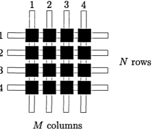
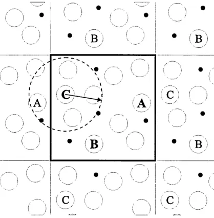
addressing, which is schematically depicted in Fig. 1.7. In this, matrix of transparent conducting rows and columns interconnects all LCD pixels. In the switching process, a voltage +Vr is applied sequentially to each row. Then, pixels in this row are switched in parallel by applying voltages ±.VC to the corresponding columns. The pixels are switched to “on” or “off” states depending on the total voltage applied, i.e. Vr ± Vc. Thus, it is very important that pixels have some switching threshold value, otherwise the applied column voltages Vc would erroneously switch pixels in other rows. This approach is also limited by the fact that in an N row display, over a given time frame t, each pixel receives its full voltage over the time period

tf = t/N. In this class of multiplexed addressing, M x N pixels can be addressed using M + N different lines.

1 2 3 4

M columns

Figure 1.7: Sketch of the multiplex addressing in LCDs.

[image:26.614.226.379.456.587.2]

or by using the active addressing approach considered below.

A thin film transistor (TFT) is put next to every pixel in the active addressing technology. TFTs maintain the state of pixels and update them only when cor­ responding rows are being accessed. The voltage across each pixel is maintained by storage capacitors which are located next to each TFT. Thus, the manufactur­ ing process needed for active addressing technology is much more complicated than that used to implement passive matrix technology, because an active transistor and a capacitor is required next to each pixel. Despite this, use of TFTs in commercial displays is widespread because they give high contrast ratios, fast switching times and high resolutions.

1.4 Bistability

Bistability is a property of a LC device by which the LC can reside in two or more distinct stable configurations under the same external conditions. Provided that these two stable LC configurations are optically distinct, e.g. form black and white in a bistable reflective display. There are two main benefits of bistability for display applications:

• Reduced power consumption. Bistable displays consume energy only when switching process occurs between two states and, consequently, do not use any energy to hold a static image. Conventional monostable displays require a constant power for their operation, but they usually require less energy for switching between optically distinct states. Thus, if a display device does not needed to be updated frequently, then there is a significant advantage in terms of power consumption in employing the bistability. This aspect is especially pertinent to mobile held devices, such as electronic book readers.

• Unlimited multiplexing capabilities. Bistable pixels do not require a contin­ uously applied voltage over some threshold to retrain a static image. As a result, they can be used with cheaper passive matrix technologies which can potentially support an arbitrary number of rows. Thus, very high resolutions can be easily achieved, as compared to TN technology, where very complex active matrix addressing needs to be used.

CHAPTER 1. INTRODUCTION 14

switch between states. Bistable twisted nematics [21] is another example, which has one state homogeneous and the other with a 360° twist; switching between these is achieved using voltages with different threshold values. Cholesteric LCD’s [2 2] have two stable states, which are a planar twisted state and a state with a focal conic texture; switching between these is achieved by electric field pulses of different lengths.

Below we consider two of the relatively recent developments in this area, namely the zenithal bistable device (ZBD) and post aligned bistable nematic (PABN). These both employ complex alignment surfaces to achieve their bistability.

1.4.1 Zenithal Bistable Device (ZBD)

The zenithal bistable device (ZBD) uses an asymmetric grating on one of the cell’s surfaces to obtain bistability [23]. A schematic illustration of the ZBD cell is depicted in Fig. 1.8. Here, both surfaces are treated so as to impose local homeotropic alignment. There are two stable states in the ZBD device, which are called the defect state (planar) and the continuous state (vertical). Depending on the pitch to groove ratio, the ZBD cell can be made to favour the planar state only, the vertical state only or both states bistably. The final case is the one used when producing devices.

(a) (b)

Figure 1.8: Sketch of ZBD stable configurations, (a) planar state (b) vertical state.

1.4.2 Post Aligned Bistable Nem atic (PABN)

The post aligned bistable nematic (PABN) device [24] uses an array of 3-dimensional posts on one of the cell sides to achieve bistability. When posts are low, the system favors only planar configurations and when posts are high, only tilted states are stable. For some intermediate post heights, however, both states are stable.

Switching between the two stable states is achieved using sign-dependant pulses. In these, a LC with negative dielectric anisotropy is usually employed, Ae < 0. The driving mechanism behind the switching is not yet fully understood, although it is assumed that flexoelectricity is involved and that the switching process involves creation and annihilation of defects [18]. We describe our study of the PABN device operation in more detail in §6.

1.5 Basics of Mesh-free M ethods

As their name suggests, the main idea behind mesh-free methods is that they do not rely on a grid. This is a big advantage over traditional grid-based methods since it fully eliminates the computational cost associated with mesh creation. In mesh- free methods, then, the spatial domain and its boundaries are represented by a set of scattered nodes without any specified intra-connectivity. As such, any confining geometry can be represented very accurately, even if the shape functions utilised within the mesh-free method are of low order.

Many types of mesh-free methods have been devised so far. The different classi­ fications of these are set out in the extensive reviews which have been published in a number of books [25, 26]. Depending on the details of their formulation procedures, mesh-free methods can be classified into three categories: those based on weak- forms, those based on collocation techniques (also called strong form) and mesh-free particle methods.

Strong-form methods are usually easy to implement, computationally efficient and have the advantage that the procedure they use for discretising PDEs is straight­ forward. In these, the numerical error is minimised on the simulation points them­ selves. The biggest issue preventing collocation methods from becoming more pop­ ular is their inability to handle derivative boundary conditions. Another issue with strong-form methods is that they have a tendency to be unstable, especially when the final solution contains high-frequency modes.

CHAPTER 1. INTRODUCTION 16

This integral operation effectively smears out the numerical error, resulting in the discretised system being more accurate and stable. The only disadvantage of weak- form methods is their decreased computational efficiency, which arises due to the numerical integration procedure outlined above.

1.5.1 Mesh-free Particle M ethods

Mesh-free particle methods (MPMs) can be seen as a certain sub-set of mesh-free methods, in which a finite set of particles is used to represent the state of a sys­ tem [27]. These particles can represent some discrete physical objects (e.g., atoms) or they can represent parts of the continuum problem domain (e.g., when solving a PDE).

MPMs can be classified into three different categories based on length scales, which are atomistic, mesoscopic and macroscopic. Classical examples of atomistic MPMs are molecular dynamics and Monte Carlo methods, in which each particle typically represents an atom. Dissipative particle dynamics (DPD) [6, 7], direct simulation Monte Carlo (DSMC) [28, 29] etc. can be seen as examples of mesoscopic MPMs. Macroscopic MPMs include smoothed particle hydrodynamics (SPH) [9, 10], Particle-in-Cell [30], Reproducing kernel particle methods (RKPM) [31] and others.

There is also a second classification of MPMs based on the mathematical model employed. This divides MPMs into deterministic and probabilistic classes. Many MPMs are probabilistic in its nature, such as DSMC, DPD etc. In deterministic techniques, on the other hand, once all initial conditions have been set, the particle’s position and properties at later simulation stages can be exactly predicted based on physical laws governing the system. Some MPMs can belong to both classes, such as SPH. SPH was originally presented as a probabilistic technique, but now it is widely used as a deterministic mesh-free particle method.

1.5.2 Consistency, Completeness and Reproducing Condi­

tions

The consistency condition is used in the analysis of finite-difference approxima­ tions. It states that a scheme L^u = f is consistent (accurate) with the differen­ tial equation Lu = f to order p, where u is any sufficiently smooth function, if

||Lu — Lhu\ \ = 0(hp). In this definition, h is the distance between the nodes in the regular FDM grid. It is easy to see that the approximation error ||Lu — Lhu\\ goes to zero when p > 0 and h —» 0.

The consistency condition is difficult to apply to mesh-free methods, where there are no predefined connections between the randomly distributed nodes and the node spacing h is not clearly defined. Thus, the reproducing condition (or completeness) is usually used in the analysis of mesh-free methods.

The reproducing condition (or, alternatively, completeness) states that an ap­ proximation uh{x) is complete to order p if polynomials up to order p can be repro­ duced exactly. This can be illustrated by considering uh(x) as being approximated by a sum of certain basis functions, i.e.

uh{x) = ^ ®i(x )uh (!-3)

i

where &i(x) are basis functions and Ui are nodal values. If the values of ui are set according to some polynomial of order p, then uh(x) should reproduce this polyno­ mial exactly. For example, if in one dimension, the nodal values are given by the polynomial

ui = a0 + aixi + a2xj + ... + apxp, (1.4)

then the reproducing condition of order p is met if

uh(x) = ^ 2 &i{x )ui = ao + a\X + a2X2 + ... + apxp. (1.5)

1

Consideration of an arbitrary choice of the coefficients, a*, then leads to the following set of conditions on the basis functions:

^ $ j ( a ; ) = l, ^2 $i{x)x i = x , . .., ^2 ^ J(x)xpI = xp. (1.6)

1 1 1

The set of basis functions {$/} also satisfies what is called the partition of unity (PU) of order p. For instance, the PU of order 0 satisfies $7(2;) = 1.

C H A P T E R 1. INTRODUCTION 18

of the first derivative yields:

= 0, ^ ® i , x ( x )x i = 1> •••> ^ 2 ^ i , x{x)xpi= p x p~1. (1.7)

i i i

Chapter 2

Landau-de Gennes Theory of

Liquid Crystals

2.1 Introduction

2.1.1 The Nem atic Order Parameter

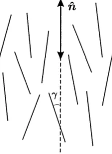
[image:33.613.242.354.489.642.2]

Quantitatively, the behaviour of LCs is best described using the concepts of the di­ rector and the associated order parameters [1]. In the nematic phase, the molecular axes of a LC tend to point along a preferred direction, called the director. The direc­ tor is denoted by a unit vector n pointing along the average molecular orientation, as sketched in Fig. 2.1. The directions ft and —n are usually equivalent and indistin­ guishable; that is why the vector n is drawn with two arrows in Fig. 2.1. Generally, the director is a function of both space and time coordinates, i.e. ft = fi(x,t).

Figure 2.1: A schematic illustration of molecular axis around the average alignment direction.

The degree of LC alignment can be described quantitatively using the scalar S',

CHAPTER 2. LANDAU-DE GENNES THEORY OF LIQUID CRYSTALS 20

which is called the order parameter. Formally, this order parameter is a second-rank quantity, but this detail is not pertinent to the remainder of this Thesis. In order to define the order parameter, we consider some sample of a LC, e.g. that depicted in Fig. 2.1. If 7 is the angle which a given molecule’s long axis makes with the director, then the degree of order can be quantified via the set of even Legendre polynomials of cos 7, averaged over an appropriate volume. Odd Legendre polynomials average to zero in uniform bulk nematic due to the head-tail symmetry of the phase. The leading non-zero number of this set is, therefore, the second averaged Legendre polynomial. This is also called the microscopic order parameter:

S = (P 2(c o s 7 )) = i ( 3 c o s 2 7 - 1), (2.1)

in which (...) denotes the statistical average and, thus, this equation can be equiv­ alently rewritten in the continuum form such as

S

=

^

J

(3 cos27 — l) f{-i)dV, (2.2)

where /(q ) is the statistical distribution function of the molecular angle 7. The function / (7) is even and periodic due to the head-tail symmetry of the phase, i.e. / ( 7 + Tf) = / ( 7 ) .

In a perfectly ordered fluid where all molecules are ideally aligned with the director, i.e. all angles 7 = 0 and the order parameter is equal to 1. In an isotropic fluid, conversely, all molecules are randomly oriented, so (cos27) = 1/3 and the order parameter is equal to 0. When all molecules lie in the plane perpendicular to the director, the order parameter S = —1/2. Although mathematically it is possible to have a negative S', in real systems the order parameter usually takes values 0 < S < 1, with typical values for a nematic being around 0.6. This order parameter is usually sufficient to describe systems composed of molecules possessing cylindrical or rotational symmetry around their long axes.

2.1.2 The Biaxiality

Molecules, in practice, do not usually have axes of complete rotational symmetry. Systems composed of such molecules, thus, might not have an axis such that rotation around it will leave the system’s state unchanged. Sometimes, this can also be the case for systems composed of uniaxial molecules. Such systems are called biaxial

can always be identified, with the third axis I being always perpendicular to these two, I = n x rh. In these, each axis has a reflection symmetry, i.e. ft —* —ft, rri —> —771 and I —>• —I.

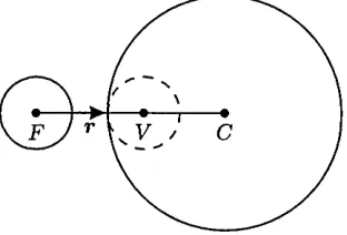
A uniaxial arrangement of both uniaxial and biaxial molecules is easy to imag­ ine, as well as the biaxial arrangement of biaxial molecules. A biaxial arrangement of uniaxial molecules is more complicated, and this situation is pertinent to defects in nematic liquid crystals. The latter situation is illustrated in Fig. 2.2, where the ordering of molecules is different depending on the axis along which the system is viewed. The distinct feature of this configuration, when viewed from the “top” in the xy-plane, is that the projections of molecules are ordered. We call the associated order parameter S2 the biaxial order parameter, which is equal to | (sin27 cos 2 7 ).

There is also a third order parameter, S3(x,t), which is related to Si(x,t) and

6 2(0?, t). For example, in the uniaxial case one of these order parameters will nor­ mally be zero and two others will be equal to each other, e.g. Si = S2 and S3 = 0.

y

> x

A ft

x

I J W /

Figure 2.2: A schematic illustration of a biaxial arrangement of uniaxial molecules viewed along three different principle axes.

Thus, in order to fully describe a biaxial system, two directors, n ( x ,t) and

77i(x, t), and two corresponding order parameters, S(x, t) = f t ( a s , t) and Pb(&, t) =

ft(cc,t), should be defined. The directors can be represented by three Euler angles, namely zenithal angle 6, azimuthal angle <p and another zenithal angle 'ip for the second director. Using the assumption that all directors are of unit length, we can then represent them using Euler angles as

ft = (cos 0 cos 4>, cos 6 sin </>, sin 6),

7Ti = (sin (p cos 'ip — cos (p sin 7p sin 9, — sin (p sin ip sin 9 — cos (p cos ip, sin ip cos 9).

CHAPTER 2. LANDAU-DE GENNES THEORY OF LIQUID CRYSTALS 22

independent variables, which are

6(x,t), 0(sM), Si(x,t), S2(x,t). (2.3)

However, there can be problems with theories based on Euler angles. For instance, when the zenithal angle 9 = 7r/2, then the azimuthal angle is undefined. Thus, extra care should be taken when solving differential equations based on this descrip­ tion.

2.1.3 The Tensor Order Parameter Q

In this subsection we describe an alternative approach for describing a nematic system, which removes problems associated with descriptions based on Euler angles. In this, instead of defining the five independent variables listed in eq. (2.3), a matrix

Q

is constructed which includes all of the information about the nematic state. This matrix is the second rank, traceless, symmetric tensor

Q

which can be written in terms of previously defined directors and order parameters as

S P \

Qa(3 ~2 (3hafi/3 ^a/?) H y^a^/3 ^qT^!3j • (2-4)

In the uniaxial state, the biaxiality Pb is equal to zero and

Q

is simplified as

Qaf3 = (3fiafig ^a/3) • (^'^)

The eigenvalues of the matrix

Q

described by eq. (2.4) are S, —1(5 + Pb) and — | (5 — Pb). In the isotropic state, all of these eigenvalues are equal to zero and

Q =

0. Since

Q

is symmetric and traceless, it contains five independent variables fully describing the nematic system. But, unlike the Euler description, which is also described by five independent variables, it is free of the description problem noted in §2.1.2.

While

Q

describes the level of microscopic ordering in LCs, there is also an intimate connection between

Q

and macroscopic quantities such as the dielectric and magnetic susceptibility, refractive index and conductivity. This provides a number of experimental ways of determining

Q.

Various techniques based on the above macroscopic quantities provide comparable results, with a maximum difference of 10% [1].

and by making it traceless we obtain:

-|(xn

- Xx)

Axcj3 3

(xil

— Xx) (2.6)

|(X|| - Xx) /

Normalisation of the above equation with the maximum anisotropy A xmaa: = (x|| —

Xl) /S gives the following form for Q:

The tensor order parameter regarded in this way does not contain any assumption on the microscopic structure of the LC under consideration. It also provides a straightforward connection between changes in microscopic ordering and variation of the associated macroscopic quantity.

2.1.4 The Nem atic-Isotropic Phase Transition

The nematic-isotropic phase transition in LCs is weakly first order. This type of transition is characterised by a discontinuous change in the order parameter at the critical temperature. Phenomenologically, we follow Landau [33] in describing this by using the Taylor expansion of the free energy density / in powers of the tensor order parameter

Q.

This expansion is usually written near

Q

= 0 as [1]

where fiSO is the free energy density of the isotropic fluid. The coefficients A, B

and C are all temperature dependant, but usually the coefficients B and C are set to be independent of temperature, while the coefficient A is chosen to depend on temperature as A = a(T — T*), where a > 0 and T* is the temperature at which the isotropic state becomes unstable. All terms in equation (2.8) for the free energy density are invariant under rotations and reflections of coordinate axes, as they should be, since the symmetry of the phase needs to be preserved. Normally, eq. (2.8) for free energy is truncated at the fourth-order terms, which provides a general description effectively representing the uniaxial phase [34]. In order to match notations, we rewrite the above Landau-de Gennes form of the free energy

.max (2.7)

CHAPTER 2. LANDAU-DE GENNES THEORY OF LIQUID CRYSTALS 24

density in the form equivalent to that given in [14]:

f L d G { Q) = fi s o T ^ ^ F Q a p Q / 3 a PfQocpQ P 'y Q j a T 'IfF Q a p Q /3 a Q fiu Q u fi' (^*9)

Here, op, (dp and 7p are the Landau-de Gennes coefficients. Thus, equation (2.9) is our main working equation for the free energy density of a thermotropic LC. It can be readily used to predict the preferred phase of the material, i.e. isotropic, uniaxial or biaxial.

We now proceed to the analysis of eq. (2.9). For this, we insert the uniaxial order tensor definition given by eqs. (2.5) into eq. (2.9), which yields:

fu a iS , T) = f iso+ a (T - T*) 52 - B S3 + C S \ (2.10) where a(T — T*) = B = ~ ~ and C = By calculating the first order derivative dfLdG(S,T)/dS, setting it to zero and solving the obtained equation with respect to 5, three stationary points are found:

5 = 0, (2.11)

s =

_L

( z b + y/9B2 — 32aC (T — T*)J , (2.1 2)

3B - — 32aC (T — T*) \ . (2.13)

Examination of the second order derivative d2fLdG(S,T)/dS2 leads to the following conclusions about these stationary points:

• 5 = 0, the LC is in the isotropic state. This phase is stable for T > Tin =

T* + metastable for T* < T < Tin and unstable for T <T*.

• 5 = ( sB + y/QB2 — 32aC(T — T*)^j, the LC is in the nematic state. It is stable for T < Tin, metastable for Tin < T < T** = T* + and not defined for T > T**.

• 5 = g^ ( sB — y/9B2 — 32aC (T — T*)^, this state is metastable with a neg­ ative 5 value for T < T*, unstable for Tin < T < T** and not defined for

T > T**.

nematic phase becomes unstable at T** and in the latter case the isotropic state becomes unstable at T*. Fig. 2.3 shows the S dependance of the free energy density for different temperature values, according to eq. (2.1 0), where all troughs can be clearly seen.

250

200

*3 ₁₅₀

100

>> 50 tan 'JU

u

a>

H 0

CD

0) £ "SO

= T T — T

-100

- 0.4 - 0.2 0 0.2 0.4 0.6

Uniaxial Order Parameter S

Figure 2.3: The dependance of the free energy density on the order parameter for various temperatures.

The order parameter given by eq. (2.12) is plotted in Fig. 2.4 as a function of temperature, where the discontinuity at T — T** can be clearly seen. It should be

a

.3 ’3 0.2

- 6 -4 - 2

-1 0 8 0

T — Tim (K)

Figure 2.4: The dependance of equilibrium order parameter S on the temperature for a set of Landau coefficients suitable for 5CB [14].

CHAPTER 2. LANDAU-DE GENNES THEORY OF LIQUID CRYSTALS 26

of

Q

were neglected in this expansion. Thus, formally this theory should be applied only in situations where S does not take large values. However, as it can be seen from Fig. 2.4, the theory provides reasonable values of order parameter deep in the nematic phase. Thus, in this thesis we apply this theory without any limitations, since we work only in the nematic phase (S ~ 0.6).

A nematic LC prefers to remain in an undistorted state with

Q

remaining uniform throughout the sample. Various external influences, such as boundary conditions, may, though, produce spatial variations in ordering. But the LC returns to the undistorted state once these external influences have been removed. This tendency can be explained through a free energy density fo, also called the distortional or elastic energy density, associated with distortions which depends on the spatial derivatives of

Q.

Derivatives of

Q

are assumed to be weak, provided that the characteristic length scale associated with changes in

Q

is much longer than the molecular dimensions. A linear expansion yields the free energy density:

where / 0 is the energy of the undistorted LC, Laig7 controls distortions correspond­ ing to a chiral nematic phase and represents the nematic elasticity. The elastic free energy density should be the same when described in different frames of reference, i.e. it should be invariant to arbitrary rotations or translations. This implies that not all of the combinations of

Q

derivatives are allowed and, in fact, the elastic free energy (2.14) can be reduced to:

where Pch denotes the helix pitch. Although there are seven third-order terms in Q, we keep only one in order to prevent having undefined constants [15], i.e. to remove the degeneracy in elastic constants when mapping them from

Q

tensor to experimental values Ka in the Frank energy approach. The elastic parameters Li

2.2 Static Theory of Liquid Crystals

2.2.1 Elasticity

Id — Jd

(dQ)

— fo + L a p j d ^ Q a p +

are related to the Prank elastic constants by the following identities [35]:

K n = - f (2 ii + L2 + L3 - SoLt), (2.16)

(2.17)

71^33 — —~ (2 L i L 2 + L z 4- 2 S o L i ), (2.18)

(2.19)

where So is the uniaxial order parameter at which the experimental measurements of the elastic constants were taken and is not necessary equal to the current equilibrium order parameter S of the LC. The saddle-splay contribution K 2a is a divergence term and does not influence the bulk behaviour. However, if the anchoring is weak at the surface, this term may contribute to surface ordering and thus change the bulk ordering.

2.2.2 Electric and M agnetic Fields

LCs interact strongly with externally applied electric and magnetic fields. The response of LCs to magnetic fields is relatively simple and depends only on the anisotropy of the magnetic susceptibility. Electric fields, on the other hand, produce many physical effects in nematics in addition to that due to dielectric anisotropy [1]. Below we consider the influence of both fields separately.

M agnetic Fields

LCs are anisotropic diamagnetic media and their magnetic susceptibilities are differ­ ent along the directions parallel (x||) and perpendicular (x_l) ^ e LC director. In nematics, the difference Ax = X|| — X jl is usually positive. If an external magnetic field H is applied to a LC sample, then the magnetisation M induced by H can be written as:

where Xa/3 is expressed following eq. (2.7). The free energy density due to the applied magnetic field can then be derived from eq. (2.2 0):

A x maxQapHp + 0^0X77fiapHp,

Ala fioXapHp (2.20)

CHAPTER 2. LANDAU-DE GENNES THEORY OF LIQUID CRYSTALS 28

In the above equation the second term is independent of the ordering. The first term, on the other hand, explicitly contains the

Q

tensor and it is minimised when the director is collinear with the applied magnetic field (for positive

Ax)-Electric Fields

In order to describe the effect of electric fields, we consider an ideal situation of a static electric field E applied to a nematic LC. In this simple set-up, two different physical processes take place. The first is due to the dielectric anisotropy and it is very similar to the effect of the diamagnetic anisotropy described above. The second effect is more complicated and arises in deformed nematics where a sponta­ neous dielectric polarization appears. This is the so-called flexoelectric effect and we consider it in the next section.

The derivation for the dielectric anisotropy effect is very similar to that for the diamagnetic anisotropy. The dielectric anisotropy Ae = e\\— ej_, where e\\ and e± are the dielectric constant measured along and perpendicular to the nematic axis, can be positive or negative depending on the structure of the constituent molecules. If an electric field E is applied to a nematic LC, then the electric displacement D has the following form

Da = eoeapEp = - A e maxQaf3Ep + -eo e^SapEp. (2.22)

The free energy density due to the electric field is then given by:

fE = ~

J

D - dE = - | e 0A - jU e77£ 2. (2.23)

For LCs with a positive anisotropy, i.e. with those having ey — ej_ > 0, the lowest energy state is when the director is parallel to the applied electric field and, thus, the molecules align along the field. In case of the negative anisotropy, ey — e± < 0, the lowest energy is achieved when the director is perpendicular to the electric field.

(2.24)

need to be solved: ✓

Da = ^a p E p , Ep = - dp4>, V x E = 0,

where 4> is the electric potential (voltage) and aj is the free charge which is in this thesis assumed to be always equal to zero. Strictly speaking, Maxwell’s equations

{daB a = 0, V x H = 0) need also to be solved for magnetic fields for higher accuracy.

2.2.3 Flexoelectricity

In some liquid crystals a splay or bend distortion can create a spontaneous dielectric polarisation which is equivalent to a local electric field. An applied electric field, on the other hand, may induce distortions which will induce a corresponding polarisa­ tion. This effect is called flexoelectricity and it was first discovered by Meyer [36]. In order to quantify this, the most general form of polarisation Pq is constructed which is proportional to the first-order spatial derivatives of the director [1]:

Pe = enhed^h^ + e33n7d7n0, (2.25)

where en and e33 are flexoelectric coefficients with the dimensions of an electric potential. There are no flexoelectric terms arising from second order derivatives due to symmetry principles. Whereas eq. (2.25) includes only the derivatives of the director, a more general expression accounting for order parameter can be written as [37]:

Pe = CidjQoj + C2Qe1dllQlil. (2.26)

CHAPTER 2. LANDAU-DE GENNES THEORY OF LIQUID CRYSTALS 30

Matching this equation with that by Meyer (2.25) provides the following relations between flexoelectric coefficients:

f 35oCi , 3S02C ^ . (Z S0C, 3S$C2\

= [ — + ^ r ) ' 633 = [ ~ 2 ---4 ~ ) • (2-28)

The free energy density due to the flexoelectric contribution has the following form:

ffiexo = —EoPe = —C\Eq8 1Qq1 — C2EoQo1dltQ*1ll. (2.29)

There is an effect similar to flexoelectricity, which is called the order electric effect [38]. It happens when there is a spatial gradient in the ordering S and there are no significant variations of the director. The polarisation in this case is found by again substituting

Q

from eq. (2.5) into eq. (2.26) with assumption that S is a variable and ft is constant. This yields

„ ( SCi , 3C25 ^ a a a 0 , ( Cx , C2S \ a c

Pe — ( ~2“ ^-4— ) nenn^nS + I — — H— — J deS. (2.30)

2.2.4 Boundary Conditions and Anchoring

When liquid crystal molecules are close to a solid boundary they experience an influence which is dependent on type of the boundary treatment. For example, a boundary treated by rubbing can impose a preferred direction of the director. In some cases, boundaries can also change th