Particle Swarm Optimization based Economic Dispatch
of Kerala Power System
K. Pramelakumari
Associate Professor Electrical and Electronics
Engineering
Government Engineering College, Thrissur
V. P. Jagathy Raj, PhD
Professor
School of Management Studies Cochin University of Science and
Technology, Kochi-22
P. S. Sreejith, PhD
Professor and Dean Faculty of Engineering Cochin University of Science and
Technology, Kochi-22
ABSTRACT
The economic load dispatch problem aims at controlling the committed generating unit outputs so as to meet the required load demand at minimum operating cost while satisfying the power demand and system equality and inequality constraints. The economic load dispatch is a non-linear constrained optimization method whose complexity increases when constraints such as system power balance constraints and generator constraints are considered. This paper describes the use of particle swarm optimization algorithm in finding out which combination of generators should be worked together in order to meet the required load demand at minimum operating cost
Keywords
Economic load dispatch, particle swarm optimization and power balance constraints.
1.
INTRODUCTION
In economic dispatch, the objective is to calculate the output power of every generating unit, for a single period of time, so that all the demands are satisfied at the minimum cost, while satisfying different constraints of the model. Optimization is a nonlinear mathematical model of a real-world problem. In this paper, particle swarm optimization technique is utilized for economic load dispatch problem to find the generating units that minimize the generation cost while satisfying a set of constraints.
The major qualitative factors in power industry are frequency, voltage and stability. In the integrated environment, it is not possible to take a corrective action by Kerala to modify the grid frequency [1]. This will be more acute when the Southern Region is integrated to the rest of India through 800kV links. Voltage and stability are within the control of the grid operators, transmission and distribution managers, where optimization is possible. The cost aspect lies in the domain of system operators in the regulated power market. Since the hourly consumption of power is several thousands of MW even a single paise per MW saves several crores of Rupees to Kerala power economy [2].
The cost of supplying electricity to consumers can be divided in to demand costs and energy cost, compared to the common industrial classification of fixed and variable costs. Demand costs are the capacity related costs for generation, transmission and distribution and vary with the quality of plant and equipment and the associated investment. Energy costs are those which vary directly with the quantity of units generated [3].
This paper focuses on an economic dispatch of Kerala power system by the formulation of cost optimization problem and finding out solution through particle swarm optimization. The data collected from Kerala State Electricity Board Ltd., are used for the model representation which portrays a real physical problem. The data consists of varying operational and maintenance costs of different generators per hour on daily basis as well as hourly load generated from 50 generators in 17 stations across the State.
2.
KERALA POWER SYSTEM: THE
NEED FOR OPTIMISATION
The cost of power procurement alone works out at present 70% of the total revenue requirement of Kerala State Electricity Board Ltd (KSEB Ltd) depending on the availability of monsoon. This necessitates for framing an optimization strategy in the management of power system. To meet the increase in energy demand the KSEB Ltd has been heavily depending on the short-term market and energy exchanges, because new major hydel projects have not yet been materialized in the State due to various reasons. At present about 15 to 20% of the energy requirement of the State is being met from short-term market i.e., high dependence on costlier power [4]. Water is the only commercially viable source for power generation within the State to ensure reliability of supply as well as energy security addition in Kerala. The need for equipping Kerala Power System to meet the demands of the excepted explosive growth in the industrial sector is well recognized.
The cost of generation and power purchase are increased on account of the reduction in hydel availability and the consequent increase in demand and excessive energy prices of short-term markets, transmission constraints on importing power from outside the State, increase in cost of liquid fuel stations etc.
During 2016-17 the total capacity addition from all sources was 55.03MW. Total installed capacity of power in the State as on March 2017 is 2,961.11MW. Of which, hydel contributed the major share of 2,107.96 MW (71.19 %); while 718.46MW was contributed by thermal projects, 59.27MW from wind and 75.42MW from solar [5]. During 2017-18 the total installed capacity in Kerala was 2791.25MW. Of which KSEB Ltd contribution was 2215.24MW and others 576.01MW.
was 2099.345 MW. The remaining 940.655MW was purchased. For this purchase Rs 16.931crore was required for one day. That is, the KSEB Ltd was running at a loss. For reducing this loss, the imported power has to be reduced by using the optimization techniques.
3.
ECONOMIC LOAD DISPATCH
PROBLEM FORMULATION
The complex nature of generation of electricity signifies ample opportunity of improvement towards the optimal power generation solution. The demand of power system varies throughout the day and reaches a different peak value from one day to another. To satisfy this demand, to start-up and shut-down, a number of generating units at various power stations each day is needed [6]. The difficult task is to decide when and which generating units are to turn on and turn off together with minimizing the total cost. Similarly, the total generation must be equal to the forecasted demand of electricity. For reducing the generation cost, optimized scheduling for economic load dispatch is necessary. Thus, the economic dispatch is one of the most important problems to be solved in the operation and planning of a power system.
The primary objective of the electric power generation is to schedule the committed generating unit outputs so as to meet the required load demand at minimum operating cost while satisfying all unit and system constraints [7]. Extensive amount of power is drawn daily from external sources that are not under the authority of Kerala power system, despite the load being much lesser than the installed capacity. Hence, this economic dispatch formulation tries to reduce external import of power and attempts to introduce self-sustainability into Kerala power system.
In the traditional economic dispatch problem, the cost function for each generator has been approximately represented by a single quadratic function and is solved using mathematical programming based on the optimization techniques [8]. Lagrange Relaxation (LR) method is commonly used to solve large scaled unit commitment problems. LR has been successfully applied to the complex unit commit problem including various hard constraints (ramp rate constraints, minimum up and down time, etc.). Unit commitment is a nonlinear mixed integer optimization problem. It schedules the operation of the generating units as minimum operating cost satisfying the demand and other constraints. [9]
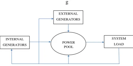
Based on the data obtained from KSEB Ltd and the Kerala State Electricity Regulatory Commission, the required parameters are made into an economic dispatch model. Figure 1 depicts the system structure of the proposed method.
[image:2.595.54.278.621.732.2]g
Fig .1: Power system structure
3.1
Objective Function
The objective function of the economic dispatch problem can be expressed in the following equation:
(1) The generation cost function is usually expressed as a quadratic polynomial as in the equation (2) [10].
(2) Where,
- Number of internal generators - Load dispatch of generator at time t - Cost coefficients of generator
Each generating unit has a unique production cost defined by its cost coefficients. Here the curve fitting method is used in order to find the cost coefficients by giving input as matrices of load in MW and cost in Rupees per hour. Curve fitting tool in MATLAB is used to obtain the value of cost coefficient.
3.2
Constraints
The objective function in equation (1) is minimized subjected to a set of constraints. The various constraints to be considered in the economic dispatch problem are: system power balance constraints and generator constraints. The major constraints considered are the following:
a) System power balance constraint is mathematically expressed as:
(3)
Where,
- the scheduled optimal generation of unit.
- the number of generators available for generating the load.
- the active power load at time point t.
- the estimated loss at time point, t.
b) Generator constraint is expressed as in the equation below:
(4)
Where,
- the minimum load generated from unit. - the maximum load generated from unit.
4.
PARTICLE SWARM OPTIMIZATION
The Particle Swarm Optimization (PSO) algorithm was introduced by Kennedy and Eberhart in 1995. The original objective of this technique was to mathematically simulate the social behavior of bird flocks and fish schools. For developing the simulation was to model human social behavior, which is not identical to fish schooling or bird flocking. In PSO [11]-[13] the potential solutions, called particles, "fly" through the problem space by following some simple rules. All of the particles have fitness values based on their position and have velocities which direct the flight of the particles. PSO is initialized with a group of random particles (solutions), and then searches for optima by updating generations. In every iteration, each particle is updated by following two "best" values. The first one is the best solution (fitness) the particle has achieved so far. This value is called “pbest” or the
individual particle best. Another "best" value that is tracked by the particle swarm optimizer is the best value obtained so far by any particle in the population. This best value is a global best and called “gbest” or the global best among all the EXTERNAL
GENERATORS
INTERNAL GENERATORS
SYSTEM LOAD POWER
considered particles, considering the current as well as all the previous iterations. After finding the two best values explained above, the particle updates its parameters, velocity and position with following equations (5) and (6):
(5)
Where, is the inertia coefficient which slows velocity over time; is the nth particle velocity after the kth iteration; is the current nth particle position in the search space;
and are the"personal" or individual best (describe the individuality) and global best (describing the social nature of the particle); and rand2 random numbers between (0,1); and are learning factors. The stop condition is usually the maximum number of allowed iterations for PSO to execute or the minimum error requirement. As with the other parameters, the stop condition depends on the problem to be optimized [14].
A total 50 generators are considered and particle of size 30 is selected. Also, a matrix of size 50×30 is initialized. For each of these generators, pbest and gbest are found in each iteration. Cost per unit is selected as pbest for each of the particles. The constraints explained in the system such as a) and b) are considered while optimizing the cost of production in each iteration. The algorithm used for this optimization includes the following steps:
Step 1: Read internal generation available for time t. Here 50 major generating stations are taken as internal generators as explained;
Step 2: Read cost coefficients that has been calculated beforehand using curve fitting tool;
Step 3: Initialize particle size, number of iteration and maximum error, learning
factors ( ) and inertia weight ( ). Define initial velocity and position of particles for each generating unit;
Step 4: Calculate dispatch and cost per unit and select cost per unit as pbest;
Step 5: Check maximum minimum conditions of dispatch from each unit;
Step 6: Select gbest (minimum of cost per unit);
Step 7: Update particle parameters;
Step 8: Calculate new dispatch and cost per unit and update
pbest;
Step 9: Check maximum and minimum conditions of dispatch and update gbest;
Step 10: Check and enforce pattern of internal and external generations; and
Step 11: Increment time slot.
Go to step 9.
In this work, PSO with time varying inertia weight (PSO-TVIW) factor is used. The optimal solution is improved by varying the value of inertia weight from 0.4 to 0.9. The entire methodology is summarized as a flow chart in figure 2.
START
SET TIME = 1 READ POWER SYSTEM DATA
OUTPUT RESULTS FETCH LOAD
DATA FOR T
INITIALIZE PARTICLE SIZE (P) FOR PSO-TVIW
INITIALIZE POSITIONS AND VELOCITIES
CALCULATE DISPATCH & COST PER UNIT (CoU) SET PARTICLE SET, P = 1
IF P<Pmax P = P +1
SET Min(CoU) AS GLOBAL BEST (GBEST) SET CURRENT CoU AS PARTICLE BEST (PBEST)
UPDATE PARTICLE PARAMETERS
CALCULATE NEW DISPATCH & CoU
IF P<Pmax
UPDATE PBEST P = P +1
IF GBEST<NEW
Min (CoU) GBEST = NEW Min (CoU)
IF Max(VELOCITY)
< TOL. CHECK & ENFORCE
CONSTRAINTS
YES
NO
YES
NO
YE S
NO NO YES
INCREMENT TIME
Fig.2: Flow chart for PSO based economic load dispatch
Table.1: Cost function coefficients of 50 units system
Generating
Units Rs/hr Rs/MWhr Rs/MWhr2 P_Optimal
1 1744.7236 0 0.0000490787 99.404936
2 1835.7919 0.00387579 0.0000930924 99.404936
3 1056.9862 0.006459667 0.0001356974 99.404936
4 1843.3758 0.001937896 0.0002987879 99.404936
5 1562.3592 0.001937896 0.000409986 99.404936
6 1027.5404 0.001937896 0.000459206 99.404936
7 1208.4982 0.0019479356 0.0009618129 42.055934
8 1476.8815 0.0038958706 0.0014026736 42.055934
9 1887.5068 0.0038958706 0.0017053512 42.055934
10 1894.8885 0.0038958706 0.001776971 42.055934
11 1087.6130 0.0038958706 0.0008436269 45.879201
12 1900.5927 0.003895876 0.0011952770 45.879201
13 1887.1669 0.000481958 -0.0001607599 2.6762867
14 1415.3756 0.002891467 -0.0059924722 2.6762867
15 1730.2804 0.00192764237 -0.0036757594 2.6762867
16 1071.8863 0.005799594728 0.0004526858 45.879201
17 1351.7612 0 0.0015765130 45.879201
18 1845.7355 0.00231983787 0.0023847449 45.879201
19 1722.2073 0.022905835 -0.0007750620 13.381433
20 1889.4924 0 -0.000473742972 13.381433
21 1585.7407 0.0152705575 -0.00007071814 13.381433
22 965.71167 0.00416582519 -0.00034552462 19.116334
23 1779.1293 0 -0.0027212523 28.674501
24 1863.9932 0 -0.00226187310 28.674501
25 1608.7351 0.0005671898 -0.00415059163 3.8232667
26 1687.7401 0.0017015687 -0.00876417201 3.8232667
27 1673.1324 0.0017015687 -0.0017019061 3.8232667
28 1322.2270 0 -0.0016889454 5.7349001
29 1585.4778 0.00226875857 -0.0080733552 5.7349001
30 1101.1866 0.0034031377 0.0049812530 5.7349001
31 1636.0469 0.0064610707 -0.0016276787 9.1758403
32 961.83284 0.00403816887 -0.00883832794 9.1758403
33 1206.9229 0.000470438 -0.00126463984 9.1758403
34 976.1713 0,0001974298 0.000739784736 9.1758403
35 1027.1317 0.0010349637 0.000201753141 12.234453
36 1753.4578 0.00075270098 0.000472815265 12.234453
37 1624.8286 0.00019742978 0.0008590879 6.1172268
38 1247.0994 0 0.0001993692 6.1172268
39 1880.2220 0.00019742978 0.000562894 6.1172268
40 964.44608 0.001579438368 0.0001062650 6.1172268
41 1368.7443 0.0001237119 -0.0001188750 12.234453
42 1311.5584 0 0.0001604344 13.763760
43 1695.5167 0 -0.0004649355 13.763760
44 1725.1999 0.00983596057 0.0002980414 13.763760
45 1116.8726 0.0009437548 0.0002663307 19.116334
46 1419.7644 0.0005243078 0.000277830 19.116334
47 1375.5862 0.0020972317 0.000435668 19.116334
48 1576.3130 0.0029361237 0.0000163413 38.232667
No. of
Days April,2015 Actual Power (Hydro)MW
Optimised power
(Hydro)MW Demand/Consumpti
on (MW)
Import power (MW)
Optimised cost (Rs.)
Cost of imported power (Rs.)
Cost saving (Rs.)
1 583.375 1869.294 2348.833542 1765.458542 41722642.08 155925298.4 114202656.3
2 696.9483 1884.776 2577.406667 1880.458367 42068200.32 166082082.9 124013882.6
3 707.0006 1895.793 2586.229792 1879.229192 42314099.76 165973522.2 123659422.4
4 726.7267 1900.361 2588.342917 1861.616217 42416057.52 164417944.3 122001886.7
5 805.2898 1871.402 2608.727292 1803.437492 41769692.64 159279599.3 117509906.6
6 780.9167 1894.732 2571.4375 1790.5208 42290418.24 158138797.1 115848378.8
7 1108.91 1960.7286 2869.769792 1760.859792 43763462.35 155519136.8 111755674.4
8 691.1335 1911.06 2517.737708 1826.604208 42654859.2 161325683.7 118670824.5
9 509.6863 1911.991 2344.18625 1834.49995 42675639.12 162023035.6 119347396.5
10 772.0631 1898.427 2562.854792 1790.791692 42372890.64 158162722.2 115789831.6
11 813.3913 1885.964 2663.89125 1850.49995 42094716.48 163436155.6 121341439.1
12 897.6962 1879.037 2680.905 1783.2088 41940105.84 157493001.2 115552895.4
13 987.4973 1892.007 2870.472292 1882.974992 42229596.24 166304351.3 124074755
14 987.4973 1918.799 2729.893125 1742.395825 42827593.68 153888399.3 111060805.6
15 1046.674 1909.516 2792.194792 1745.520792 42620397.12 154164396.3 111543999.2
16 929.3985 1873.7701 2642.231875 1712.833375 41822548.63 151277443.7 109454895
17 1065.873 1947.4246 2834.908125 1769.035125 43466517.07 156241182.2 112774665.2
18 811.3067 1908.314 2519.056667 1707.749967 42593568.48 150828477.1 108234908.6
19 658.4935 1881.351 2372.264375 1713.770875 41991754.32 151360243.7 109368489.4
20 710.1985 1887.489 2520.136042 1809.937542 42128754.48 159853683.7 117724929.2
21 821.3923 1910.71 2652.996458 1831.604158 42647047.2 161767279.3 119120232.1
22 815.155 1838.3188 2831.83125 2016.67625 41031275.62 178112846.4 137081570.8
23 1014.736 1901.868 2756.902917 1742.166917 42449693.76 153868182.1 111418488.3
24 995.3971 1883.575 2766.355417 1770.958317 42041394 156411038.5 114369644.5
25 1046.156 1893.948 2792.760625 1746.604625 42272919.36 154260120.5 111987201.1
26 1004.426 1872.152 2764.321458 1759.895458 41786432.64 155433966.9 113647534.2
27 1096.679 1902.131 2578.4675 1481.7885 42455563.92 130871560.3 88415996.4
28 1098.085 1907.211 2804.772708 1706.687708 42568949.52 150734658.4 108165708.9
29 1148.448 1911.751 2879.8225 1731.3745 42670282.32 152914995.8 110244713.5
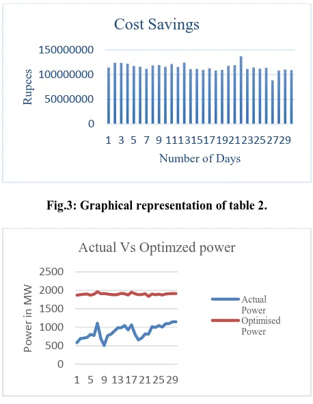
[image:5.595.56.570.74.567.2]30 1149.784 1914.541 2869.700833 1719.916833 42732555.12 151903054.7 109170499.6
Table.2: The optimum cost corresponding to optimum scheduling for the month April 2015
5. RESULTS AND DISCUSSION
5.1: Case I - PSO based hourly economic
scheduling and cumulative daily optimal
cost evaluation
The implementation of the PSO algorithm and problem formulation is done using MATLAB. Short term and mid-term load of the month April 2015 data is used for getting optimum cost withPSO. The load for the time slot of 00.30hrs to 24.00hrs of is considered. Table 1 shows the cost coefficient values of of 50 generators and the optimum generated load. In this study, the steps of the algorithm explained above are implemented by using the load of 1st April 2015 in one hour and the results are shown in the
table 1. The cost per unit of internal generation is 93 paise per kWhr and cost per unit of imported power is rupees 3.68 per
kWhr respectively. From the results obtained, it can be found that hydro generation can be increased by 57.68% and import of power can be reduced by 63.72%. Thus, there is a daily saving of Rupees 1356475.92 per hour.
5.2:Case II - PSO based hourly economic
scheduling and cumulative monthly optimal
cost evaluation
cost corresponding to optimum scheduling of April 2015. Fig 4 shows the optimum power corresponding to actual power which is inferred from the table 2.
Fig.3: Graphical representation of table 2.
Fig. 4: Graphical representation of actual and optimized power.
6. CONCLUSION
In this paper, the cost optimization of Kerala power system based on economic load dispatch has been done. The PSO is used as a tool for solving the economic load dispatch problem. PSO-TVIW based optimum scheduling with STLF (for one day and one month) data has been carried out. The algorithm used in this program and the results in each are described in detail. Half-hourly economic scheduling and cumulative daily and monthly optimal cost evaluation and steps involved in monthly cost calculation are also described. It is clear from the result that the actual expenditure occurred in KSEB Ltd is higher than that obtained by using PSO. That means, the total production cost of KSEB Ltd can be minimized by applying PSO-TVIW.
5.
REFERENCES
[1] Economic Review, 1997, State Planning Board, Government of Kerala.
[2] Lee, K. Y., Y. T. Cha, and J. H. Park. "Short-term Load Forecasting Using an Artificial Neural Network."IEEE Transactions on Power Systems 7, no. 1 (1992): 124-132. [3] Wood, Allen J., and Bruce F. Wollenberg. Power Generation, Operation, and Control. John Wiley & Sons, 2007.
[4] Kerala State Electricity Regulatory Commission Orders, April 2017
[5] Economic Review, 2017, State Planning Board, Government of Kerala.
[6] Jaini, A., I. Musirin, N. Aminudin, M. M. Othman, and TK A. Rahman. "Particle Swarm Optimization (PSO) Technique in Economic Power Dispatch Problems." In Power Engineering and Optimization Conference (PEOCO), 2010 4th International, pp. 308-312. IEEE, 2010.
[7] Hamdan, Norhamimi, Musse Mohamud Ahmed, and Ismail Hassan. "New Costs Optimization Concepts for Unit Commitment and Economic Load Dispatch in Large Scale Power Systems." In TENCON 2004. 2004 IEEE Region 10 Conference, vol. 100, pp. 480-483. IEEE, 2004.
[8] Dasgupta, Koustav, and Sumit Banerjee. "An Analysis of Economic Load Dispatch Using Different Algorithms." In Non-Conventional Energy (ICONCE), 2014 1st International Conference on, pp. 216-219. IEEE, 2014. [9] Ahmed, M. M., and I. Hassan. "Costs Optimization for
Unit Commitment and Economic Load Dispatch in Large Scale Power Systems." In Power and Energy Conference, 2004. Proceedings. National, pp. 190-194. IEEE, 2004. [10] Gaing, Zwe-Lee. "Particle Swarm Optimization to
Solving the Economic Dispatch Considering the Generator Constraints." IEEE Transactions on Power Systems 18, no. 3 (2003): 1187-1195.
[11] Eberhart, Russell, and James Kennedy. "A New Optimizer Using Particle Swarm Theory." In Micro
Machine and Human Science, 1995.MHS'95.,
Proceedings of the Sixth International Symposium, pp. 39-43. IEEE, 1995.
[12] Hu, Xiaohui, and Russell Eberhart. "Solving Constrained Nonlinear Optimization Problems with Particle Swarm Optimization." In Proceedings of the Sixth World Multiconference on Systemics, Cybernetics and Informatics, vol. 5, pp. 203-206. 2002.
[13] Eberhart, Russell C., and Yuhui Shi. "Guest Editorial Special Issue on Particle Swarm Optimization." IEEE Transactions on Evolutionary Computation 8, no. 3 (2004): 201-203.
[14] Lee, Kwang Y., and Mohamed A. El-Sharkawi, eds. Modern Heuristic Optimization Techniques: Theory and Applications to Power Systems. Vol. 39. John Wiley & Sons, 2008.
[15] Park, J. H., Y. S. Kim, I. K. Eom, and K. Y. Lee. "Economic Load Dispatch for Piecewise Quadratic Cost Function Using Hopfield Neural Network." IEEE Transactions on Power Systems 8, no. 3 (1993): 1030-1038
0 50000000 100000000 150000000
1 3 5 7 9 11 13 15 17 19 21 23 25 27 29
Ru
p
ee
s
Number of Days
Cost Savings
0 500 1000 1500 2000 2500
1 5 9 13 17 21 25 29
Po
w
er
in
MW