Early Prediction of Software Defect using Ensemble Learning: A Comparative Study

Early Prediction of Software Defect using Ensemble

Learning: A Comparative Study

Ashraf Sayed Abdou

Department of Information Systems and

Technology,

Institute of Statistical Studies and Research,

Cairo University, Egypt

Nagy Ramadan Darwish

Department of Information Systems and

Technology,

Institute of Statistical Studies and Research,

Cairo University, Egypt

ABSTRACT

Recently, early prediction of software defects using the machine learning techniques has attracted more attention of researchers due to its importance in producing a successful software. On the other side, it reduces the cost of software development and facilitates procedures to identify the reasons for determining the percentage of defect-prone software in future. There is no conclusive evidence for specific types of machine learning that will be more efficient and accurate to predict of software defects. However, some of the previous related work proposes the ensemble learning techniques as a more accurate alternative. This paper introduces the resample technique with three types of ensemble learners; Boosting, Bagging and Rotation Forest, using eight of base learner tested on seven types of benchmark datasets provided in the PROMISE repository. Results indicate that accuracy has been improved using ensemble techniques more than single leaners especially in conjunction with Rotation Forest with the resample technique in most of the algorithms used in the experimental results.

Keywords

Software Defects, Ensemble methods, Resample Technique, Base Learner, Bagging, Boosting, Rotation Forest.

1.

INTRODUCTION

The huge investment and money spent in development of software engineering causes an increase the cost of maintenance of software systems [1]. Nowadays, the huge size of the developed software is becoming more and more complex. Also, a large size of program codes. For that, the probability of having software defects has been increased and quality assurance methods are not sufficient to overcome all software defects in huge systems. Therefore, the identification of which modules in the software most probably to be defective, it can help in reducing the limited resources and time of development [2]. Numbers of predictive models are proposed in this research to predict of the defects in software modules by using several types of classifiers such as Decision Tree [3], SVM [4], ANN [5] and Naïve Bayes [6]. The classification model, including two categories of software defects: Fault-Prone (FP) software and Non-Fault-Prone (NFP) software. The objective of the research is to utilize the ensemble learning methods that combines multiple single learners by using the different subset of features to improve the accuracy of the predictive model. Another advantage of ensemble methods, it the enhancement of the performance by using different types of classifiers together because this reduces the variance between them and keeps the bias error rate without increasing. Three types of ensemble learners are utilized [7]: Bagging, Boosting and Rotation Forest techniques [8]. Bagging technique depends on subsampling the training dataset by replacing samples and generates training subsets, then combining the results of different

classifiers based on a voting technique. Boosting technique is focusing on misclassified training samples that are relearning with several weight values according to the accuracy of classified samples, and then it applies a linear combination to get the final decision from the outputs. Rotation Forest technique uses a features extraction method to split it to a number of subsets features, and then uses the Principle Components Analysis (PCA) on each subset separately with different rotation to produce a new set of the extracted features that preserve the information of scattering data, and it increases the accuracy of each built individual classifier. The researchers build a framework for the comparative study to measure the accuracy of experiments in a different scale of 7 public datasets provided in the NASA repository as a benchmark dataset [9]. The researchers applied another type of statistical measure it called “paired t-test” because it is very helpful to measure and simulate the results of the same algorithm more than once. The experiment test will be applied in the public domain dataset to observe the difference between mean values within the experimental measures.

The rest of this paper is organized into five sections. Sec 2 presented the related work. Sec 3 will reviews a background of different ensemble techniques and its advantage. Sec 4 is devoted to the experimental results and discussion. Conclusion and future work are given in section 5.

2.

RELATED WORK

Ensemble methods have been utilized to address data imbalance problems and it can handle a small-sized dataset. Sampling-based online Bagging method has been proposed by Wang et al. [10] as a type of ensemble learning approach. In their experiments study, if the class distribution changed dynamically over time, then the sampling based on the online Bagging will be unstable in their performance. In the normal situation without these changes, sampling achieves a balanced performance. To address this problem, in case of dynamic changes, authors introduce the under-sampling technique that is robust against samples and work well in case of dynamic changing in class distribution. A Roughly Balanced Bagging (RBBAG) algorithm, proposed by Seliya et al. [11], as a different type of solutions based on ensemble learning. The experiment results measured by the Geometric Mean (GM), indicated that RBBAG method is more effective in performance and classification accuracy than individual classifiers such as C4.5 decision tree and naive Bayes classifier. In addition, RGBBAG has the ability to handle imbalance data it occurs in the test data.

experiment results show that the one-against-one coding schema achieves the best results.

A comparative study of ensemble learning methods related to software defect has been proposed by Wang et al [13]. The proposed model included Boosting, Bagging, Random forest, Random tree, Stacking and Voting methods. The author compares the previous ensemble methods with a single classifier such as Naive Bayes. The experiment of the comparative analysis reported that the ensemble models outperformed the result of the single classifier based on several public datasets.

Arvinder et al [14], proposed using ensemble learning methods for predicting the defects in open source software. The author uses three homogenous ensemble methods, such as Bagging, Rotation Forest and Boosting on fifteen of base learners to build the software defect prediction model. The results show that a naïve base classifier is not recommended to be used as a base classifier for ensemble techniques because it does not achieve any performance gain than a single classifier.

Chug and Singh [15] examined five of machine learning algorithms used for early prediction of software defect i.e. Particle Swarm Optimization (PSO), Artificial Neural Network (ANN), Naïve Bayes (NB), Decision Tree (DT) and Linear Classifier (LC). The results of the study show that, the linear classifier is better in prediction accuracy than other algorithms, but ANN and DT algorithms have the lowest error rate. The popular metrics used is the NASA dataset such as inheritance, cohesion and Line of Code (LOC) metrics. Kevin et al [16] introduced oversampling techniques as preprocessing with a set of the individual base learner to build the ensemble model. Three of oversample techniques have been employed to overcome the bias of the sampling approach. Then, ensemble learning is used to increase the accuracy of classification by taking the advantage of many classifiers. The results of experiments show that the ensemble learning with resampling technique improved the accuracy and reduced the false negative rate compared to the single learner. Ahmed et al [17] presented the machine learning approach such as Neural Network, Fuzzy Logic, Linear and Logistic Regression to predict the failure of a software project. The author used multiple linear regression analyses to determine the critical failure factors, then it employed the fuzzy logic to predict the failure of a software project.

3.

BACKGROUND

Ensemble learning is called meta-learning techniques that integrate multiple classifiers computed separately over different databases, and then it builds a classification model based on weight vote technique to improve the prediction of the software defect [18]. One of the advantages of using these techniques is it enhances the accuracy of defect prediction model compared to a single classifier.

In ensemble technique, the results of a set of learning classifiers, whose individual decisions are combined together, enhance the overall system. Also, in ensemble learning, different types of the classifiers can be combined into one predictive model to improve the accuracy of prediction, decrease bias (Boosting) and variance (Bagging). On the other side, the ensemble techniques have classified into two types: parallel ensemble and sequential ensemble techniques. In case of parallel ensemble technique, it depends on the independence among base learners such as Random Forest (RF) classifier that generates the base learner in parallel to

reduce the average of error dramatically. Another type is called sequential ensemble learning which depends on the dependence among the base learners. Such as AdaBoost algorithm, which is used to boost the overall performance by assigning a high weight to mislabeled training examples. In the comparative study, several classification models have been used such as an Artificial Neural Network (ANN) and Support Vector Machine (SVM) as discriminating linear classifiers. Random Forest (RF) and J48 as decision tree classifiers, Naïve Bayes as a probabilistic classifier and PART algorithm are used as a classification rules algorithm. The results of these methods are compared to ensemble techniques such as Bagging, Boosting and Rotation Forest to examine the effectiveness of ensemble methods in the accuracy of the software defect prediction model.

3.1

Single Machine Linear Classifiers

3.1.1

Artificial Neural Network (ANN)

ANN is a computational model of a biological neuron. The basic unit of ANN is called a neuron [19]. It consists of several nodes and it receives the inputs of an external source or from other nodes, each input has an associated weight. The results of neural network transformed into the output after the input of weight are added. In this research, the researchers utilized a Multi-Layer Perceptron (MLP) technique, which is considered one of the feed-forward neural networks, and it uses the back-propagation algorithm as a supervised learning technique.

3.1.2

Support Vector Machine (SVM)

SVM is considered one of a new trend in machine learning algorithm; it can deal with nonlinear problem data by using Kernel Function [20]. SVM achieve high classification accuracy because it has a high ability to map high dimensional input data from nonlinear to linear separable data. The main concept of SVM depends on the maximization of margin distance between different classes and minimizing the training error. The hyperplane is determined by selecting the closest samples to the margin. SVM can solve the classification problems by building a global function after completing the training phase for all samples. One of the disadvantages of global methods is the high computational cost is required. Furthermore, a global method in sometimes cannot achieve a sufficient approximation because no parameter values can be provided in the global solution methods.

3.1.3

Locally Weighted Learning (LWL)

The basic idea of LWL [21] is to build a local model based on neighboring data instead of building a global model. According to the influence of data points on prediction model, each data point in the case of the neighborhood to the current query point it will have a higher weight factor than the points very distant. One advantage of LWL algorithm, it is the ability to build approximation function and easy to add new incremental training points.

3.1.4

Naïve Bayes (NB)

The Naïve Bayes classifier [22] depends on the Bayes rule theorem of conditional probability as a simple classifier. It assumes that attributes’ values are independent and unrelated, it called independent feature model. Naïve Bayes uses the maximum likelihood methods [23] to estimate its parameters in many of the applications.

3.1.5

Decision Tree: Random Forest (RF)

individual tree with a few features. Then, many of small and weak decision trees are built in parallel. Finally, majority voting or average techniques have applied to combine the trees and form a single and strong learner.

3.1.6

J48 Decision Tree

Decision tree J48 [25] uses the concept of information entropy to build decision tree from a set of labeled training examples. J48 used to generate a pruned or un-pruned tree by applying of the C4.5 algorithm. J48 split the data into a smaller subset and examines the difference in entropy (normalized information gain) that’s the output of the selected attribute used for splitting the data. After that, it makes a decision of the classification based on the attribute with the highest information gain.

3.1.7

Logistic Regression (LR)

The Logistic Regression algorithm [26] is used to predict the output of categorical dependent variable (binary) from a set of independent variables (predictor) and it is considered a type of the regression analysis in the statistic. It performs the classification based on the transformation of the target variable to assume any binary values in the interval. Logistic Regression finds the weight that fits the training examples well, and then it transforms the target using a linear function of predictor variables to approximate the target of the response variable.

3.1.8

PART Algorithm

PART algorithm [27] is a combination of both RIPPER and C4.5 algorithms; it used a method of the rule induction to build a partial tree for the full training examples. The partial tree contains the unexpected branches and subtree replacement has been used during building the tree as a pruning strategy to build a partial tree. Based on the value of minimum entropy, PART algorithm expands the nodes until it finds the node that corresponds to the value provided or returns null if it finds nothing. Then, the process of the pruning is started. The subtree replaces the node by one of its leaf children when it will be the better. The PART algorithm follows the separate-and-conquer strategy based on a recursive algorithm.

3.2

Ensemble Machine Learning

Classifiers

3.2.1

Bagging Techniques

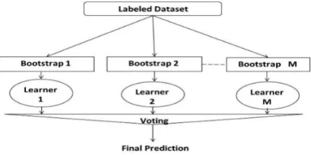
Bagging technique is one of the ensemble learning techniques [28] and it is called also Bootstrap aggregating Bagging, as shown in Fig 1, it depends on the different training sizes of training data it called bags collected from the training dataset. Bagging method is used to construct each member of the ensemble. Then, the prediction model is built for each subset of bags, and it combines the values of multiple outputs by taking either voting or average over the class label. First, Bagging algorithm selects a random sample with replacement from the original training dataset, and then multiple outputs of learner algorithms are generated (bags). Finally, Bagging algorithm applies the predictor on the samples and combine the results by voting techniques and predicts the final class label for software defect.

Fig. 1 Bagging Technique

3.2.2

Boosting algorithm

Boosting Technique [29] is depends on sequential training model and in each round the new model is trained. First, the Boosting algorithm performs multiple iterations on the training samples to construct an aggregated predictor. Then, the weight of incorrectly training instances will be increased after each iteration to force learning algorithm to focus on incorrect instances than instance correctly predicted.

Finally, the classifiers are combined by using the voting technique to predict the final result of defect prediction model as shown in Fig 2.

Fig. 2 Boosting Technique

3.2.3

Rotation Forest

Rotation Forest [30] is a new classifier of ensemble methods, it works according to the following steps: First, dividing the training data features based on random split into features subset by using a feature extraction method. Second, for each subset of features, the Bootstrap technique is used to build training subset of training samples. Third, a Principal Components Analysis (PCA) technique is used on each training subset to rotate the coordinate axes during the transformation process and it retains all of the principle components without discarding. Finally, the training subsets will be applied to the base learner of the same type and the average of the prediction of the base learner will be the final output.

4.

PROPOSED MODEL

Fig. 3 Resample Techniques

The oversampling technique is used to adjust the class distribution of a dataset. The resampling techniques classified into two types: oversampling and under-resampling techniques as shown in Fig 3. The oversampling technique increase the size of the training set and therefore the training time of the model will be increased but it doesn't lose the information.

The under-resampling technique decreases the time of training, but its loss of information.

Fig. 4 Comparative Study of Software Prediction Model

In the oversampling, it must have enough information in the minor class and it must not lose the valuable information in the major class. To decide which one is better, two parameters must be taken into consideration; distribution of data in imbalanced dataset, and imbalance ratio that shows the degree of imbalance. In the proposed model, the researchers used oversampling techniques because it can balance the class distribution and it is more suitable for the case study. The objective of this phase is to manipulate the training dataset to rectify the skewed class and handle non-uniform distribution to overcome the biased problem. Random subsamples of training data are produced by resampling filter in two cases: one without replacement and another with replacement. In the first case, each selected item will be removed once it selected of the full dataset and it cannot be selected again. By using the resample method with replacement technique, each the

selected item can be selected more than once.

(3) Classification Stage: in this stage, the ensemble classifier for classification model has been built by using the combination of the results of multiple classifiers into a single software by using Aggregating, Bootstrap and Rotation Forest techniques [32] to increase the performance of the overall software defect model. On the other side, the researcher's test differed types of a single classifier before and after applying the preprocessing phase to measure the effect of the resampling technique on accuracy. (4) Comparison Study: The last stage is used to compare the results of ensemble methods against the results of a single classifier with different performance measures and different size of datasets.

5.

EXPERIMENTAL

RESULTS

AND

DISCUSSION

5.1

Dataset Description and Research

Hypothesis

In this research, the researchers selected seven benchmark datasets with different sizes of a number of modules to perform the experiments using the PROMISE repository [33]. The description of the dataset is shown in table1 that includes: number of modules, code attribute, and defective modules. Table 1: Description of datasets used in the study

Project Name

Number of Code Attribute

Number of Modules

Number of Defective Modules

MC2 40 161 52

MW1 38 403 31

KC3 38 458 43

CM1 38 505 48

KC1 21 2107 325

PC1 38 1107 76

PC4 38 1458 178

These datasets contain static code measures [34] such as Design Density, McCabe’s Cyclomatic complexity, Halstead, LOC, etc. The main metrics classified into two main categories code and design metrics. The researchers present in table 2, numbers of attributes of matrices are used in MDP, and these metrics are depending on the degree of complexity and product size. The software is classified to defect-prone if the number of defects in software class greater than zero, otherwise it is called free defect prone. The software metrics stated in table 2 as independent variables and the associated dependent variable for a defect prone. Since the main target of this study is to measure the effects of ensemble learning techniques to increase the software defect prediction accuracy according to the following hypothesis:

H0 (Null Hypothesis): in this case, if do not find any difference in the predictive accuracy of ensemble techniques and the base learner.

H1 (Alternate Hypothesis1): in this case, if the software prediction accuracy of the base learner has a lower predictive accuracy than the ensemble learner.

Table 2: Studied Metrics within NASA MDP datasets [35] Category Software

Metrics

Description

Code Number of Lines The number of lines in module

LOC Count The total count of line of code

LOC blank The number of blank lines in a module

LOC Comment The number of lines of comments for a module LOC Executable The number of lines of

executable code for modules Halstead Content:

µ

The halstead length content of a module

µ = µ1 + µ2

Halstead Volume: V

The halstead volume metric of a module

V = N ∗ log2(µ1 + µ2)

Halstead Length: N

The halstead length metric of a module

N = N1 + N2

Halstead Level: L The halstead level metric of a module

L = (𝟐∗µ𝟐)) µ𝟏∗𝐍𝟐

Halstead Difficulty: D

The halstead difficulty metric of a module D = 𝟏

𝐋

Halstead Effort: E

The halstead effort metric of a module E = 𝐕

𝐋

Design Design Complexity: iv(G)

The design complexity of a module

Cyclomatic Complexity: v(G)

Cyclomatic Complexity: v(G) = e − n + 2

Design Density Design density is calculated as: 𝐢𝐯(𝐆)

𝐯(𝐆)

Branch Count Branch count metrics

Condition Count Number of conditionals in a given module

Essential Complexity: ev(G)

The essential complexity of module

Edge Count: e Number of edges found in a given module control from one module to another Node Count: n Number of nodes found in a

given module

Essential Density Essential density is calculated as: (𝐞𝐯(𝐆)−𝟏))

(𝐯(𝐆)−𝟏)

Maintains Severity

Maintenance Severity is calculated as: 𝐞𝐯(𝐆)

𝐯(𝐆)

5.2

Experimental Procedures

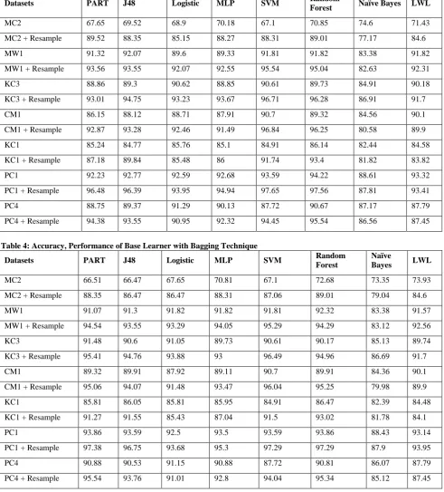
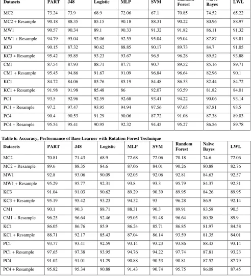
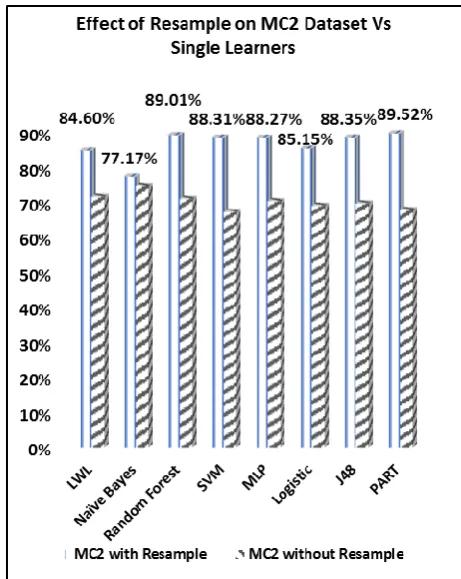
The outcomes of several single base learners are embedded by using the different types of ensemble techniques to enhance the accuracy better than using a single base learner. Based on the previous summary of MDP dataset, the researchers use 8 base learners and three ensemble techniques as presented in section 3. The experiments results were implemented on an Intel Core (TM) I7 with 16 GB RAM and Windows 10 operating system. WEKA [36] version 3.8.1 has been used for classification as a machine learning toolkit. The researchers applied the cross-validation technique to avoid sample bias problem by using the x*y way of cross-validation. The researchers select both of x and y as ten [37] which means 10- fold cross validation will repeat 10 times. The dataset was split randomly into the number of equal size partitions. The last partition is used as the test set and the remaining partitions are used as training set. The researchers conducted four experiment sets. In the first experiment, each of eight single classifiers was employed within 10-cross-validation without sign any resemble learning technique and the final outcome has been recorded twice, one by using 7 datasets before applying resample technique and another one after applying resample technique. In the second experiment, the Bagging ensemble technique embedded in each of the eight-single learner and the researchers recorded the final outcome by using 10-fold cross-validation. For example, if the Bagging is embedded with SVM learner, it is will call Bagging-SVM and all other Bagging learners were recorded with the same way twice, after and before applying resample technique. In the second experiment, the Boosting ensemble techniques embedded in each of eight single learners and the researchers recorded the final outcome by using 10- fold cross-validation. For example, if Boosting is embedded with SVM learner, it is called Boosting-SVM and the eight-base learners are recorded with 10-cross-validation after and before applying resample technique. In the fourth experiment, the Rotation Forest ensemble technique embedded in each of eight single learners and the researchers recorded the final outcome by using 10- fold cross-validation, and the eight base learners are recorded with 10-cross-validation after and before applying resample technique. The experimental procedures are shown with details in Fig 6.

5.3

Evaluation Measurements

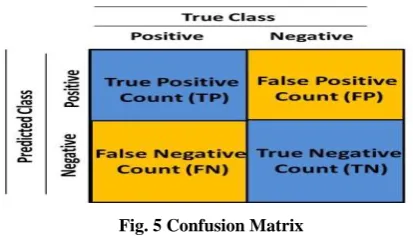
Fig. 5 Confusion Matrix

The researchers used in this study three types of evaluation measurements such as Accuracy, Recall and Area under Curve (AUC) measures. These measurements can be calculated based on the confusion matrix according to the below equations:

The accuracy is defined as the percentage of correctly classified examples against the total of examples.

The recall is defined as the fraction of relevant instances that have been retrieved over the total amount of relevant instances.

Fig. 6 Steps of Experiments Procedures

The AUC it is called an Area under Receiver Operating Characteristic (ROC) curve. That is the integral of ROC curve with a true positive rate as the Y-axis and the false positive rate at X-axis. The better generalization ability achieved if the ROC curve is close to the top-left of coordinate. For that, AUC will be larger, and the learner gets better. In the experiments, the accuracy measure has been used as a predictive measure and the comparison between Boosting, Bagging and Rotation Forest ensemble techniques with single base learner over seven of MDP benchmark datasets will be applied.

5.4

Experimental Results

The performance results of accuracy are presented in the tables, 3, 4, 5, 6. The researchers used non-parametric significance test to predict the software defects in the experiments as a statistical comparison test [38] of learners because it is highly recommended in the current research. The researchers achieve the fair and rigorous comparison of learners by using significance test [39] because of its ability to distinguish significant observation from chance observations. According to [39], Wilcoxon signed rank test is recommended as a non-parametric test to be utilized for comparing between two learners over multiple datasets. Otherwise, in case of comparing the multiple learners over multiple datasets, the fireman test is recommended by Post-hoc Nemenyi test. In this research study, the researchers performed the pairwise comparison test between Boosting, Bagging and Rotation Forest ensembles learners with their corresponding of base learners. Then, the researchers applied the Wilcoxon signed rank test to determine any statistically significant difference in accuracy between base learners and ensemble learners.

TN+TP

Accuracy=

TP+FP+TN+FN

TP

Recall=

Table 3: Accuracy, Performance of Base Learner

Datasets PART J48 Logistic MLP SVM Random

Forest Naïve Bayes LWL

MC2 67.65 69.52 68.9 70.18 67.1 70.85 74.6 71.43

MC2 + Resample 89.52 88.35 85.15 88.27 88.31 89.01 77.17 84.6

MW1 91.32 92.07 89.6 89.33 91.81 91.82 83.38 91.82

MW1 + Resample 93.56 93.55 92.07 92.55 95.54 95.04 82.63 92.31

KC3 88.86 89.3 90.62 88.85 90.61 89.73 84.91 90.18

KC3 + Resample 93.01 94.75 93.23 93.67 96.71 96.28 86.91 91.7

CM1 86.15 88.12 88.71 87.91 90.7 89.32 84.56 90.1

CM1 + Resample 92.87 93.28 92.46 91.49 96.84 96.25 80.58 89.9

KC1 85.24 84.77 85.76 85.1 84.91 86.14 82.44 84.58

KC1 + Resample 87.18 89.84 85.48 86 91.74 93.4 81.82 83.82

PC1 92.23 92.77 92.59 92.68 93.59 94.22 88.61 93.32

PC1 + Resample 96.48 96.39 93.95 94.94 97.65 97.56 87.81 93.41

PC4 88.75 89.37 91.29 90.13 87.72 90.67 87.17 87.79

PC4 + Resample 94.38 93.55 90.95 92.32 94.45 95.54 86.56 87.45

Table 4: Accuracy, Performance of Base Learner with Bagging Technique

Datasets PART J48 Logistic MLP SVM Random Forest

Naïve

Bayes LWL

MC2 66.51 66.47 67.65 70.81 67.1 72.68 73.35 73.93

MC2 + Resample 88.35 86.47 86.47 88.31 87.06 89.01 79.04 84.6

MW1 91.07 91.3 91.82 91.82 91.81 92.32 83.38 91.57

MW1 + Resample 94.54 93.55 93.29 94.05 95.29 94.29 83.12 92.56

KC3 91.48 90.6 91.05 89.73 90.61 90.17 85.13 89.74

KC3 + Resample 95.41 94.76 93.88 93 96.49 94.96 86.69 91.7

CM1 89.32 89.91 87.92 89.11 90.7 89.91 84.36 90.1

CM1 + Resample 95.06 94.07 91.48 93.47 96.04 95.25 79.98 89.9

KC1 85.81 86.05 85.81 85.95 84.91 86.47 82.39 84.48

KC1 + Resample 91.27 91.55 85.43 87.04 91.5 93.02 81.78 84.1

PC1 93.86 93.59 92.5 93.5 93.59 93.86 88.43 93.14

PC1 + Resample 97.38 96.75 93.68 95.3 97.29 97.29 87.9 93.95

PC4 90.88 90.53 91.15 90.88 87.72 90.81 86.07 87.79

Table 5: Accuracy, Performance of Base Learner with Boosting Technique

Datasets PART J48 Logistic MLP SVM Random Forest

Naïve

Bayes LWL

MC2 73.24 73.9 68.9 72.06 67.1 70.85 74.52 65.22

MC2 + Resample 90.18 88.35 85.15 90.18 88.31 90.22 80.96 88.97

MW1 90.57 90.34 89.1 90.33 91.32 91.82 86.11 91.32

MW1 + Resample 94.79 95.04 92.06 92.55 95.04 95.04 87.87 93.81

KC3 90.15 87.32 90.62 88.85 90.17 89.73 84.7 91.05

KC3 + Resample 95.42 95.85 93.23 93.67 96.5 96.28 89.52 93.88

CM1 87.54 87.93 88.71 87.71 90.7 89.52 85.16 89.71

CM1 + Resample 95.45 94.86 91.67 91.09 96.84 96.64 82.96 90.1

KC1 84.72 84.06 85.76 85.19 84.48 86.33 82.44 84.72

KC1 + Resample 91.98 91.98 85.48 86 92.07 93.59 81.82 84.01

PC1 93.5 92.96 92.59 92.68 93.41 94.22 90.06 93.14

PC1 + Resample 97.2 97.47 93.95 94.94 97.56 97.65 87.81 93.5

PC4 90.4 90.53 91.29 90.06 87.72 91.08 87.38 89.03

PC4 + Resample 95.54 95.41 90.95 92.32 94.45 95.27 86.56 89.78

Table 6: Accuracy, Performance of Base Learner with Rotation Forest Technique

Datasets PART J48 Logistic MLP SVM Random Forest

Naïve

Bayes LWL

MC2 70.81 71.43 68.9 72.68 72.06 70.18 74.6 72.06

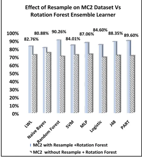
MC2 + Resample 89.6 88.35 84.6 87.06 84.01 90.26 80.88 82.76

MW1 92.8 93.06 90.09 92.05 92.06 92.81 84.63 92.57

MW1 + Resample 95.29 95.77 92.31 93.8 93.3 95.79 84.37 92.31

KC3 91.04 91.03 90.62 89.29 90.39 89.95 84.26 89.95

KC3 + Resample 95.19 95.42 93.23 94.32 93 96.28 86.9 92.14

CM1 90.1 90.3 88.71 88.31 90.3 89.91 83.58 90.5

CM1 + Resample 96.25 96.64 92.46 95.05 91.48 96.64 80.38 89.9

KC1 86.05 86.76 85.9 86.24 85.71 86.85 81.97 84.58

KC1 + Resample 88.71 92.17 85.43 87.04 86.14 93.59 81.35 84.01

PC1 93.77 93.41 92.59 93.14 93.23 93.86 88.43 93.14

PC1 + Resample 97.65 97.38 93.95 94.76 94.22 97.74 87.81 93.23

PC4 91.02 91.01 91.29 90.88 90.53 90.81 87.52 87.79

PC4 + Resample 95.82 95.34 90.88 91.43 90.74 95.75 86.08 87.45

In case of no any difference between base learners and ensemble learners it called the null hypothesis, if the p-values of the Wilcoxon statistic test is less than 0.05, the null hypothesis is rejected. Hypothesis 1 will be accepted if Wilcoxon test is significant and the accuracy, performance is “gain” by using Boosting, Bagging and Rotation Forest ensemble learners. Finally, hypothesis 2 will be accepted, if Wilcoxon test is significant and the accuracy, performance is “loss” by using ensemble learners. The comparison between the base learners and the respective ensemble learners are stated in table 7. With the results of p-values, as in table 7,

In Boosting method, there is no gain in accuracy, performance with J48, Logistic, MLP, and LWL. For that, the null hypothesis is not rejected for thesis four learners. On another side, in Boosting method, the significant accuracy of performance is gained by PART, Random Forest, and Naïve Bayes. For that, the null hypothesis is rejected and hypothesis 1 is accepted. For SVM learner, the significant accuracy of performance is a loss. So, alternative 2 is accepted and the researchers are not recommending Boosting SVM single learner. In Rotation Forest method, there is no gained in accuracy, performance with Logistic, Naïve Bayes and LWL. For that, the null hypothesis is not rejected. Also, the researchers find the significant accuracy, performance is gained by using PART, J48, MLP and Random Forest single learner. For that, the null hypothesis is rejected and alternative hypothesis 1 is accepted. Finally, just SVM learners with Rotation Forest is loss the accuracy, performance so, the alternative hypothesis 2 is accepted and the researchers are not recommending using SVM single learner with Rotation Forest ensemble method.

The best results are achieved by using Rotation Forest than Boosting and Bagging ensemble methods. Table 7 is presenting the P-values of eight base learners with 3 ensemble learning methods. The final recommendations for the best ensemble method for each one, from eight base classifiers, are stated in table 8.

Table7: Comparison of Accuracy by Wilcoxon Test Base

Learner

Bagging

Technique

Boosting

Technique

Rotation Forest

Technique

PART 0.013 (↑) 0.003 (↑) 0.001 (↑)

J48 0.249 (-) 0.142 (-) 0.001 (↑) Logistic 0.754 (-) 0.109 (-) 0.753 (-) MLP 0.003 (↑) 0.310 (-) 0.030 (↑)

SVM 0.018(↓) 0.050 (↓) 0.096(↓) Random

Forest 0.807 (-) 0.068 (↑) 0.033(↑) Naïve

Bayes 0.294 (-) 0.014 (↑) 0.875 (-)

LWL 0.441 (-) 0.158 (-) 0.441(-)

Table8: Recommended Ensemble techniques

Base Learner

Recommended ensemble Techniques

Best Ensemble Methods

PART Bagging, Boosting and Rotation Forest

Bagging, Boosting and Rotation Forest equally good

J48 Rotation Forest

Rotation Forest

Logistic None None

MLP Bagging and Rotation

Forest Bagging _{Rotation Forest} and

equally good

SVM None None

Random Forest

Boosting and Rotation Forest

Boosting and Rotation Forest equally good Naïve

Bayes Boosting Boosting

LWL None None

Table 8 shows that, in case of more than one base learner who provides significant accuracy, performance, the researchers determine which one is best by applying the pairwise comparison through the Wilcoxon sign rank test with three ensemble methods and the best ensemble method is recommended. The researchers used in this study, the public dataset for early prediction of software defects with different sizes and the results compared with the previous studies to avoid any source of biased related to the data source. As shown in figures 7, 8, 9, 10, the accuracy has been increased by using the resample technique for all base classifiers and the ensemble learning methods. The researchers analyzed the results on MC2 as a test sample.

Fig. 8: The Effect of Resample on MC2 with Boosting Method

Fig. 9: The effect of Resample on MC2 with Bagging Method

Fig. 10: The Effect of Resample on MC2 with Rotation Forest

0% 10% 20% 30% 40% 50% 60% 70% 80%

90% 84.06%79.04% 89.01%

87.06% 88.31%

86.47% 86.47%

88.35%

Effect of Resample on MC2 Dataset Vs

Bagging Ensemble Learner

MC2 with Resample + Bagging

MC2 without Resample + Bagging

0% 10% 20% 30% 40% 50% 60% 70% 80% 90% 100% _88.97%

80.96% 90.22%

88.31% 90.18%

85.15% 88.35%

90.18%

Effect of Resample on MC2 Dataset Vs

BOOSTING Ensemble Learner

MC2 with Resample + Boosting

MC2 without Resample + Boosting

0% 10% 20% 30% 40% 50% 60% 70% 80% 90% 100%

82.76%

80.88% 90.26%

84.01%87.06% 84.60%

88.35% 89.60%

Effect of Resample on MC2 Dataset Vs

Rotation Forest Ensemble Learner

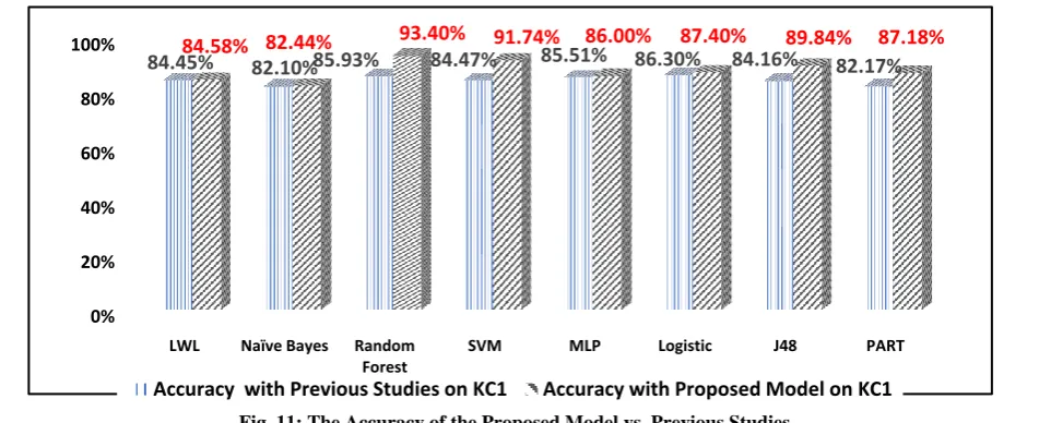
Fig. 11: The Accuracy of the Proposed Model vs. Previous Studies

6.

CONCLUSION AND FUTURE WORK

In this study, the researchers have analyzed the accuracy, performance of three ensemble learner methods Boosting, Bagging and Rotation Forest based on 8 bases single learners in the SDP dataset of software prediction defect and the results as follow:

1) The accuracy of most of the single leaners is enhanced on the most of 7 samples of NASA datasets by using the resample technique as preprocessing step and is showed in Figures 7: 10 which applied to MC2 dataset as an example in this case study.

2) The researchers do not recommend using SVM, Logistic and SVM as a single learner with three homogenous resample methods Boosting, Bagging and Rotation Forest.

3) The accuracy, performance is gained by using Bagging with MLP and PART base learner. With Boosting, the performance accuracy is gained for PART, Random Forest and Naïve Bayes Whereas Rotation Forest with 4 base learners is gained in performance such PART, J48, MLP and Random Forest.

4) The accuracy of performance results is loosed by using SVM with three of homogenous ensemble methods, with Rotation Forest, there are no accuracy, performance losses except with SVM. Thus, with Rotation Forest, there are no accuracy, performance losses except with SVM. Thus, Rotation Forest is the best method the researchers are recommended to use this research study for its advantage of the generalization ability.

5) The accuracy of proposed model using resample technique has been better than the accuracy of previous studies as shown in Fig 11, and table 9.

In the future work, more of ensemble algorithms will be compared with the different base classifier for each of software, datasets, and several of preprocessing techniques will be tested to choose best one to enhance the results.

Table 9: Comparative between Previous Studies and the Proposed Model with Resample Technique

Classification Algorithms

Accuracy with the Previous Study on KC1

Accuracy with Proposed Model on KC1

LWL 84.45% [38] 84.58%

Naïve Bayes 82.10% [37] 82.44% Random Forest 85.93% [37] 93.40%

SVM 84.47% [37] 91.74%

MLP 85.51% [37] 86.00%

Logistic 86.30% [38] 87.40%

J48 84.16% [37] 89.84%

PART 82.17% [39] 87.18%

7.

REFERENCES

[1] C. Catal and B. Diri. "A systematic review of software fault prediction studies", Expert systems with applications, Vol. 36, No. 4, 2009, pp.7346-7354. [2] Wang, and Z.Liu. "Software defect prediction based on

classifiers ensemble", Jisuanji Yingyong Yanjiu,Vol 30, No. 6 , 2013,pp.1734-1738.

[3] S. Nickolas, V. Reddy, S. Reddy and A.Nickolas "Feature selection using decision tree induction in class level metrics dataset for software defect predictions", In Proceedings of the world congress on engineering and computer science, Vol. 1, 2010, pp. 124-129.

[4] K Elish and M. Elish, "Predicting defect-prone software modules using support vector machines", Journal of Systems and Software,Vol. 81, No. 5, 2008,pp. 649-660. [5] J. Zheng "Cost-sensitive Boosting neural networks for

software defect prediction", Expert Systems with Applications,Vol. 37, No. 6, 2010, PP.4537-4543. [6] T. Wang and W. Li, "Naive bayes software defect

prediction model", CiSE, 2010, pp. 1-4.

[7] H. Wang and T. Khoshgoftaar "A comparative study of ensemble feature selection techniques for software defect

0% 20% 40% 60% 80% 100%

LWL Naïve Bayes Random Forest

SVM MLP Logistic J48 PART

84.45%

84.58% 82.44%

_82.10%85.93%

84.47%

85.51%

86.30%

84.16%

_82.17%

93.40%

91.74%

86.00%

87.40%

89.84%

87.18%

40 prediction", CMLA, 2010.

[8] H. Laradji, M. Alshayeb and L. Ghouti, "Software defect prediction using ensemble learning on selected features", Information and Software Technology,Vol. 58, 2015,pp. 388-402.

[9] S. Qinbao, Z. Jia, M. Shepperd, S. Ying, and J. Liu, "A general software defect-proneness prediction framework", IEEE Transactions on Software Engineering, Vol. 37, No. 3, 2011, pp.356-370.

[10]W. Shuo, L. Minku and X. Yao, "Online class imbalance learning and its applications in fault detection", IJCIA, Vol.12, No.4, 2013.

[11]S. Naeem, M. Khoshgoftaar and V. Hulse, "Predicting faults in high assurance software", HASE, 2010, pp. 26-34.

[12]Z .Sun, Q. Song, X. Zhu,” Using coding-based ensemble learning to improve software defect prediction”, IEEE Transactions on Systems, Vol.43, No.6, 2012, pp. 313-325.

[13]T. Wang, W. Li, H. Shi and Z. Liu, "Software defect prediction based on classifiers ensemble", JICS, Vol.8, No.16, 2011, pp.4241-4254.

[14]A. Kaur and K. Kamaldeep, "Performance analysis of ensemble learning for predicting defects in open source software", ICACCI, 2014, pp. 219-225.

[15]P. Singh and A. Chug, "Software defect prediction analysis using machine learning algorithms", In International Conference of Computing and Data Science, 2017, pp. 775-781.

[16]H.Shamsul, L.Kevin and M.Abdelrazek, "An ensemble oversampling model for class imbalance problem in software defect prediction ", IEEE, 2018.

[17]A. Abdel Aziz, N. Ramadan and H. Hefny, "Towards a Machine Learning Model for Predicting Failure of Agile Software Projects", IJCA, Vol.168, No.6, 2017.

[18]S. Wang and X. Yao, "Using class imbalance learning for software defect prediction", Vol.62, No.2, 2013, pp.434-443.

[19]H. Yuan, C. Van Wiele and S. Khorram. "An automated artificial neural network system for land use/land cover classification from Landsat TM imagery", MDPI, Vol.1, No.3, 2009, pp. 243-265.

[20]T. Kavzoglu, and I. Colkesen, "A kernel functions analysis for support vector machines for land cover classification", IJAEO, Vol.11, No.5, 2009, pp. 352-359. [21]A. Kaur, K. Kaur and D. Chopra "An empirical study of

software entropy based bug prediction using machine learning", ICDS ,Vol.8, No.2, 2017, pp. 599-616. [22]J. Chen, H. Huang, S. Tian, and Y. Qu. "Feature

selection for text classification with Naïve Bayes", Expert Systems with Applications, Vol.6, No. 3, 2009, pp. 5432-5435.

[23]C. Toon and S. Verwer, "Three naive Bayes approaches for discrimination-free classification", Data Mining and Knowledge Discovery, Vol. 21, No. 2, 2010,pp. 277-292. [24]A. Kaur and R. Malhotram, “Application of random

forest in predicting fault-prone classes”, ICACTE, Vol.8, 2008, pp. 37-43.

[25]A.Koru, and H. Liu, "Building effective defect-prediction models in practice. IEEE software”, Vol.22, No.6, 2005, pp.23-29.

[26]I. Kurt, M. Ture and Kurum, (2008). "Comparing performances of logistic regression, classification and regression tree, and neural networks for predicting coronary artery disease”, Expert systems with applications, Vol.34, No.1, pp. 366-374.

[27]E. Frank and H. Witten "Generating accurate rule sets without global optimization ", Computing and Mathematical Sciences, 1998.

[28]T, Khoshgoftaar, H. Van and A. Napolitano, "Comparing boosting and bagging techniques with noisy and imbalanced data”, IEEE Transactions on Systems, Vol.41, No.3, pp.552-568.

[29]M. Galar, A. Fernandez, E. Barrenechea, H. Bustince, and F Herrera, "A review on ensembles for the class imbalance problem: bagging-, boosting-, and hybrid-based approaches", IEEE Transactions on Systems, Man,Vol.42, No. 4 , 2012, pp. 463-484.

[30]E. Menahem, L. Rokach, and Y. Elovici, "Troika–An improved stacking schema for classification tasks", Information Sciences,Vo; 179, No. 24 ,2009, pp. 4097-4122.

[31]V. Francisco, B. Ghimire and J. Rogan, "An assessment of the effectiveness of a random forest classifier for land-cover classification", ISPRS Vol.67, 2012, pp. 93-104. [32]Y. Saeys,., T. Abeel and Y. Van, “Robust feature

selection using ensemble feature selection techniques”, In Joint European Conference on Machine Learning and Knowledge Discovery in Databases,2008, pp. 313-325. [33]Y. Ma, K. Qin, and S.Zhu, "Discrimination analysis for

predicting defect-prone software modules", Journal of Applied Mathematics, 2014.

[34]Q. Song,, Z. Jia and M. Shepperd ,"A general software defect-proneness prediction framework", IEEE Transactions on Software Engineering, Vol. 37, No..3, 2011, pp. 356-370.

[35]Y. Jiang, C. Bojan, M. Tim and B. Nick, "Comparing design and code metrics for software quality prediction, PROMISE, 2008, pp. 11-18.

[36]M. Hall, E. Mark, G. Holmes and B. Pfahringer, "The WEKA data mining software: an update", ACM SIGKDD Vol. 11, No. 1, 2009, pp.10-18.

[37]T. Menzies, J. Greenwald and Frank, "Data mining static code attributes to learn defect predictors”. IEEE Software Engineering, Vol.33, No.1, 2007, pp.2-13.

[38]J Demšar, "Statistical comparisons of classifiers over multiple data sets. Journal of Machine learning research”, 2006, Vol.7, pp.1-30.