A model of bone adaptation as a topology optimization process with contact

A model of bone adaptation as a topology optimization

process with contact

António Andrade-Campos, António Ramos, José A. Simões

Department of Mechanical Engineering, Centre for Mechanical Technology & Automation, University of Aveiro, Campus Universitário de Santiago, Aveiro, Portugal

Email: [email protected]

Received 7 January 2012; revised 22 February 2012; accepted 2 March 2012

ABSTRACT

Topology optimization is presently used in most di-verse scientific, technologic and industrial areas, in-cluding biomechanics. Bone remodelling models and structural optimization has mutually provided inspi-ration for new developments in biomechanics and biomedicine. Considering that bone has the ability to adapt its internal structure to mechanical loading (Wolff’s law and Roux’s paradigm), it is possible to model the behaviour of the bone structure by the use of a topology optimization methodology whose opti-mization variables can be the relative densities and the orthotropic directions. In this work, the internal bone adaptation of a proximal femur is considered. The bone-remodelling scheme is numerically described by a time-dependent evolutionary procedure with anisotropic material parameters. The remodelling rate equation is obtained from the structural optimi-zation task of maximizing the stiffness subject to a biological cost associated with metabolic maintenance of bone tissue in time. The situation of multiple load conditions is considered for a three-dimensional finite element model of the proximal femur. The bone den-sity distribution of a real femur is used as the initial design for the onset of the remodelling mechanism. Examples of bone adaptation resulting from load changes are presented. The three-dimensional finite element model of the proximal femur with initial bone density distribution was adapted to implant a cementless stem. A remeshing technique is used to assign the bone relative density distribution to the new geometry and mesh. The time adaptation of the bone is assessed considering contact with friction at the bone-stem interface. Results of bone density evo-lution and osteointegration distribution are obtained.

Keywords:Bone remodelling; Topology Optimization;

Finite element; Contact; Osteointegration

1. INTRODUCTION

Since the works of Michell and Bendsøe and Kikuchi [1], topology optimization has become an effective design methodology to obtain lighter and efficient structures. Until today, diverse topology optimization methods have been developed and presented. The methods based on the SIMP (Solid Isotropic Microstructure with Penalization) technique, originally introduced by Bendsøe [1], have had large acceptance due to its efficiency and simplicity.

Currently, topology optimization methods are being used in biomechanics and biomedical engineering, namely in bone-remodelling schemes and bone-adaptation mod-els. Considering that bone has the ability to adapt its in-ternal structure to mechanical loads and to changes of the load environment (paradigm of Roux and/or Wolff law [2]), it is possible to mathematically model the behaviour of the bone structure through a topological optimization methodology whose optimization variable is the relative or apparent density.

Many different mathematical and phenomenological models have described the remodelling process of the internal structure of bone. These models have in common the definition of an equilibrium state based on energy levels, on stress levels or on a reference state density. Generally, these models present an equation of the evo-lution of the non-equilibrium state for the equilibrium state through the change of state variables as, for in-stance, the local densities [3]. The remodelling process occurs when the bone senses a stimulus originated from a change of external loads [2,3].

the changes of the implant-bone interface conditions. In 1993, Sadegh et al. presented a bone remodelling theory to predict the ingrowth of bone into implant cavi-ties. Considering a very small dimensional scale, the model predicted the bone ingrowth in screwed implants. More recently, Fernandes [4,5] and Bagge [3] presented models of bone adaptation of the proximal femur. Both models consider a three-dimensional finite element model that evolves as a topology optimization scheme. Although the presented models could achieve the bone density distribution, none of them consider the inclusion of a prosthetic device. Both analyses use a single hexahedral finite element geometric model.

The osteointegration1 _{process (also called osseo-inte-}

gration) over an implant surface was also investigated using a finite element model by Spears et al. in 2000. The contact interface considers contact elements that account large sliding contact movement and total bond-ing was considered possible for elements with a micro-motion of less than 40 μm.

The use of elastic springs to model the bone implant interface was introduced by Egan and Marsden in 2001. The stiffness of an interface bonding spring is progres-sively increased at the point where the deformation (proportional to the displacement) induced by the exter-nal loads remained below a given threshold.

A similar progressive interface bonding has been pre-sented by Fernandes et al. [6,7] together with the bone remodelling model of the whole femur after total hip replacement. Changes in the interface conditions in con-junction with a global optimization criterion based in Microstructural homogenisation and a cost minimization was used. Although the previous model considers not only the bonding process but also de-bonding process, the time was not correlated and the loading conditions applied were the same as the healthy bone that, for an implanted femur, does not correspond to the reality [7-9]. Additionally, the numerical solutions were obtained starting with a homogeneous solution of the trabecular bone with a relative density equal to 30%.

A purely biomechanical model, intended to predict the long-term secondary stability of the implant starting from the biomechanical stability immediately after the opera-tion, was also presented by Viceconti et al. [10-13]. This model, also compared with a simpler one [13], uses a finite element model discretized in three-dimension hexahedral elements and a continuous rule-based adapta-tion scheme as a dynamic system. Although this model describes the whole bone-implant model, it does not consider the change in the microstructural apparent den-sity of the bone that can affect the interface and overall stiffness of the bone.

A recently model for living interfaces with bone im-plants was introduced by Moreo et al. [14]. This model reproduces the evolutive behaviour of bony interfaces accounting with bone ingrowth and deterioration by means of a finite element continuum damage mechanics formulation. It was observed that stiffer stems (such as stainless steel and Titanium stems) improve the primary fixation comparing with softer ones (Polyacetal stems). Even though the results of the simulation agree reasona-bly with clinical observations, the model presented ex-hibits some limitations associated to the lack and uncer-tainly of the different model parameters.

Almost all the bone ingrowth models that use finite element analysis consider a constant finite element dis-cretization and the bone ingrowth is characterized by an increase of stiffness. Recently, Reina et al. [15,16] tried to model bone ingrowth in distraction osteogenesis con-sidering mechanical and biological factors. Although this model considers a remeshing technique that allow the creation of new elements, the analysis was limited to a two-dimension rectangular geometric model and some biological issues are not clear.

Also recently, the bone remodelling model based on topology optimization was extended to a hierarchical model by Coelho et al. [17,18]. This hierarchical model characterizes both the macro and microstructure of the bone by means of a multiscale asymptotic homogenisa-tion technique. However, this study does not consider an insertion of any prosthetic device and the implant-bone interface is not studied.

The development of biomechanical models is a hard task. The major difficulty in the development of such models is the lack of experimental quantitative results, specifically in vivo human data results. As little or no experimental methods are currently available to investi-gate the relationship between primary stability and os-teointegration in vivo, all published studies on this topic are based on numerical simulations. However, some in vivo and ex vivo observations are available for the por-tion of implant surface that has some osteo-bond but not necessary fully bonded (or fully osteointegrated) [19,20].

The objective of this work is to present a model of bone adaptation that accounts the time and the change of stimulus. These stimuli are represented by mechanical loads. In order to obtain a realistic bone remodelling simulation, the initial structure needs to be approxi-mately equivalent to a femur. Thus, a multiload topology optimization process is applied with the purpose of find-ing the optimum initial distribution of densities corre-sponding to the proximal region of a healthy femur. Dif-ferent finite element meshes are used.

The bone adaptation model is also applied in the case of an implanted femur considering the bone and implant stem surfaces in contact. The bone ingrowth process is 1_{The prefix osteo, meaning bone, came from the Greek osteo. This term,}

simulated through a numerical model able to modify the contact conditions during the remodelling process. There-fore, a global optimization criterion with contact formu-lation and bone ingrowth is used. The contact conditions are modified based on the stem-bone relative displace-ment and stresses. The numerical initial conditions were retrieved from the femur bone just before the medical surgery. A remeshing technique is employed in order to transfer the properties from the intact femur to the im-planted-femur.

2. METHODOLOGY

2.1. Material Description

Due to its porous and adaptive structure, bone presents an orthotropic behaviour whose orthotropic coefficients change with the bone region and evolve with the remod-elling process. These aspects imply that modremod-elling the bone microstructure is an extreme hard task. Many bone- remodelling models use a power-law relation between the apparent density and the isotropic elasticity modulus of cancellous bone [2]:

bone ,

n  

E E



E

(1) where E is the isotropic elasticity matrix, ρ is the density

and Ebone is the stiffness matrix of the bone structure. The

previous relation has the advantage of being simple and computationally very inexpensive, but anisotropy is not considered. The power-law relation is similar to the use of the SIMP method in the bone adaptation process.

Other bone-remodelling models use polynomial func-tions that characterize the stiffness matrix coefficients as a function of the density and can be written as [3]:



bone  f ,

E (2)

This model, which already accounts for anisotropy, considers a constant microstructure whose material prop-erties are symmetrically cubic. This approach is also computationally inexpensive.

An orthotropic material model can be obtained using homogenization methods such as, for example, the as-ymptotic homogenization method. In this method, the cancellous bone structure is idealized by a microstruc-tural cell assuming that the material can be reproduced by a periodic repetition of the cell. Taking in account the shape of the bone microstructure, the material properties are a function of the mechanical characteristics of the solid material and the volume content in the cell [21-24]:

 

 

bone cell , with

 _{ }

E x E y yx (3)

where x and y are the properties at the macro (bone) and

microscale (cell), respectively, and ε is the asymptotic homogenization constant that corresponds to the relation of the characteristic dimensions between the micro and

macroscale. The use of two scales related with a small dimension parameter corresponds to a particular applica-tion of the multiple-scale method. This method, that as-sumes a total periodicity of the cells, requires the calcu-lation of the cell microstructure properties (through a finite element analysis) for each integration point of the mac-rostructure, leading to a very computationally expensive process. Although this method considers full anisotropy, generally, the used unit cells take parallelepiped geome-tries that are quite different from the real trabecular bone microstructure, and can be considered non-realistic.

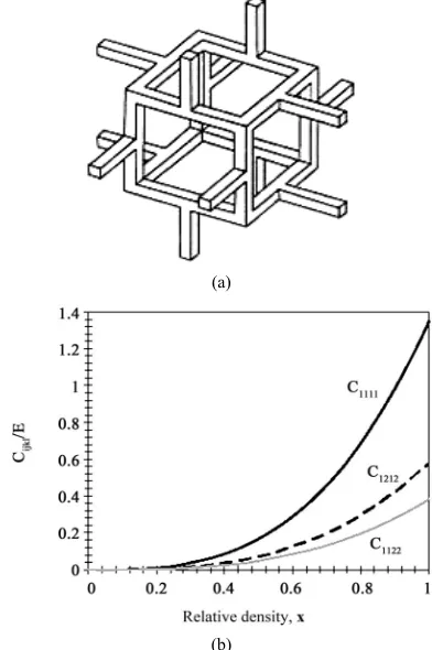
The difficulty of description of the orthotropic behav-iour of the bone material is well-known and evidenced by the numerous mentioned models. In this work, despite the disadvantages presented, the asymptotic homogeni-zation method is used. To achieve the material properties as continuous functions of the relative volume fraction, the cell structure, shown in Figure 1(a), has been used.

However, the material properties at tissue levels are as-sumed isotropic [3]. In order to decrease the CPU time required by this method, the homogenized material properties are fitted to polynomials (see Figure 1(b)).

For more details concerning the implementation of this method, see [22-24].

(a)

(b)

2.2. Bone Remodelling as an Optimization Process

The initial distribution of the apparent density of bone needs to be realistic. Therefore, it can be obtained by a CT scan (computerized tomography scan) or by stiffness maximization of the structure [3], if Wolff’s law is con-sidered. The maximization of the stiffness of a structure corresponds to the minimization of the strain energy. Assuming that bone adapts to its mechanical environ-ment, the bone remodelling process consists of the com-putation of bone relative density at each point by the solution of an optimization problem formulated in the continuum universe. Numerically, the continuum can be approximated by finite quantities. Therefore, the process of finding a reasonable structure can be an optimization task that considers the three-dimensional domain discre-tized in finite elements and whose optimization variables are the relative volume fractions x of each element.

These variables are constants in each element and take the values of 0 (void) to 1 (total density, cortical bone). The optimization process is subject to a volume con-straint and to the finite element equations for each load. The optimization problem can be defined as

 

 

1 1 1

min : Nl j j Nl j Ne e p e e

j j e _j

c w w x

       _ 







u ku (4)

with the following constraints and conditions

   

s 1

min

,

0 1, , ,

, 1, ,

e N e e e i e l j j

x V V

x x N

j N       



K U F



 .

(5)

and, in the case of multiple solids, contact conditions for the bone/stem interface

 

 

, ,

,

, ,

( ),

0, 0, 0.

n T n n

N N N n

elast s s

T T T T

T

elast s

T T T T T T

T N

u g u

t k g k u s

k k t                               

u u n u u n

u u

u u u u

t

t u u u

t           , s (6)

Πj is the strain energy for the jth load case, w represents

the weight factor and Ne and Nl are the number of ele-ments and load cases respectively. The maximum admis-sible volume and the volume in each finite element are represented respectively as V and . In each itera-tion, a finite element analysis (FEA) is performed. The global stiffness matrix K and the load vector F are

known for each load case and the global and element displacement vector, U and ue, respectively, are found.

s e V

The contact problem with Coulomb friction in Eq.6

considers a penalization approach and the inclusion of an elastic reversible term for the tangential displacements (or velocities). In this equation, the subscripts N and T denote normal and tangential properties, respectively. Therefore, tN and tT are the normal and tangential contact forces applied on the unilateral contact interface. The first expressions in 6 define the normal and tangential displacements of the contact boundary through projec-tions of the displacement u on the boundary normal n.

The function g is the actual gap between the two bodies in contact while s is the initial gap. The second line de-fines the penalisation-type constitutive equation for nor-mal traction, where the operator . represents the posi-tive value of the argument. The tangential velocity T

is divided into the elastic and sliding component (as in perfect elastoplasticity). The sliding velocity is propor-tional to the derivative of the sliding potential  defined in the last line of 6 (coulomb model).

u

The FEA can be executed with the aid of an exterior

FE program. FE programs ABAQUS® _{[25] or MSC.}

MARC® _{[26] were used in this work. In order to change}

the properties in each element, a user routine UMAT (ABAQUS 2006) was developed for the commercial program ABAQUS®_{. For the MSC.MARC}® _{a user}

rou-tine ANELAS [26] was used. The contact problem is solved using a surface-based contact model being the stem the master surface and the bone the slave surface. As mentioned, the penalty method is used for the tangen-tial contact condition.

It is assumed that the design variables x (relative den-sity) are constants within each finite element. The opti-mization problem, achieved through an iterative proce-dure, is solved using the MMA method (Method of Moving Asymptotes) [1] or the optimality criteria (OC) [1,3,27]. The OC algorithm is easy to implement and very efficient for a single constraint. For multiple con-straints, the OC cannot be used and, therefore, this is the main motivation for switching to MMA. On the standard stiffness optimization problem, the MMA can be care-fully tuned to be more efficient than the OC. However, in the standard settings they are very similar. The OC method, based in the optimum Lagrange function, uses a fixed-point updating scheme. It can be written as

1 _{, 1, ,}

k η k

e e e e,

x _B x e_{ } N

















min min

1

max 1 , if max 1 , ,

otherwise, 1, , .

min 1 ,1 if min 1 ,1 ,

k k η k

e e e e

k η k

e e e e

k k k η

e e e e

x x x B x x

x B x e N

x x x B

      _  _  _  _  _   _{     }      

 (8)

The Be parameter is defined as

s 1

, 1, ,

λ l N j e e j j e x

B w e N

V



 





where λ is the Lagrange multiplier parameter that results from the volume constraint. A local optimum is reached if Be = 1 for densities xmin < x < 1. This update scheme

adds material to areas with specific strain energy higher than λ (Be > 1) and removes it if the energy is below this value [1]. The variable η is a tuning parameter and ξ a move limit. Both η and ξ control the changes that can happen in each iteration. They can evolve with the pro-cedure in order to enhance the efficiency of the method.

The update of xe depends on the present value of the

Lagrange multiplier λ and, as a consequence, should be adjusted in order to satisfy the volume constraint. The value of λ can be found by a bi-sectioning algorithm considering that the total volume, with the actual relative densities, is a continuous and decreasing function of the multiplier λ.

If a direct implementation of a topology optimization method is made, patches of checkerboard pattern appear often in solutions. Restriction methods reduce or remove the checkerboarding in some cases, but not in all of them. With the aim of preventing the numerical problem of checkerboard, the filter method suggested by Sigmund [1] is used. In this method, the sensitivity of each element Be

is affected by the sensibilities of the neighbouring ele-ments. The change in the sensitivity is proportional to the distance between the elements. The scheme works by modifying the element sensitivities of the compliance as follows [1]: 1 mod 1 1 _ˆ . ˆ N f f N f e e f f E H x f

x _{x H}  x



 _



_





 (10)

The convolution operator (weight factor) ˆHf is

cal-culated as













ˆ _{dist , ,}

dist , , 1, , ,

f

H r e f

f N e f r e N

 

    (11)

where the operator is defined as the distance

between the centre of element e and the centre of ele-ment f. Note that the convolution operator is zero outside the filter area and decays linearly with the distance from element f. The modified sensitivities of Eq.10 are used in

the optimization problem using the OC or MMA update

method.



In the case of the bone adaptation process, the material behaviour must be formulated progressively with time. Therefore, Eq.7 is used as the remodelling rate equation

but it was considered that each iteration is a time step. Hence,

 

s , 1, ,

t

t

t t

t t e t t t

e e e e

e

x

,

e

x x B x e N

V     _   _{ }  

   (12)

where t represents the time. In the previous equation, if the Lagrange multiplier is kept constant during the re-modelling process, bone can form and resort material. Therefore, in the remodelling process, λ is denoted os-teometabolic cost and is related with the maintenance of bone mass. This parameter, 0 < λ < 5, should be depend-ent of the age, degree of bone osteoporoses, etc., i.e.,





   (13)

when the strain energy sensitivity is not in equilibrium with the element constant there is a change in the bone relative volume. In each element, a response Be

greater than the one hypertrophy is assigned and Be less

than one atrophy is assigned [3]. The equilibrium level, where no resorption or apposition takes place, is achieved when the elements with intermediate relative volume fractions have Be equal to the unity.

s

λVe

In this work, the limit of the change in volume fraction in each time increment was based on the work of Jee [28]. This author verified that it can take place a maximum bone turnover rate of 7.6%/year (≈ 0.021%/day), consid-ering a total bone loss in 13 years. As a result, if the stimuli in an element leads to a local bone changing greater than the limit, the value of Be is numerically

damped with aid of η [3]. The parameter η (0 < η < 1), that influences the sensitivity of all the elements in a proportional way in each time increment, can be found by a bisection algorithm.

2.3. Osteointegration Model

The osteointegration model intends to reproduce the ad-aptation of the bone considering the insertion of a stem. This model simulates the changes of the bone/stem in-terface conditions.



is observed. If a coated uncemented prosthesis is inserted, it is expected bone ingrowth in the coated zones after some postoperative time (see Figure 2).

In this work, a contact formulation is used together with a methodology to detect where bone ingrowth exists and evolutes. At each time increment, the contact condi-tions are updated considering a relative displacement criteria. These criteria are based on the studies performed by Fernandes et al. [6,7].

The osteointegration model aims the simulation of the bone/stem interaction. After implantation of the prosthe-sis, bone begins to attach to the coated stem wall and the prosthesis retains stability. However, bone ingrowth can be inhibited in certain zones due to high relative dis-placements.

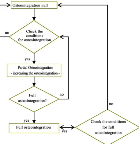
Initially, the osteointegration is considered null (see

Figure 3). In this post-operative condition, contact with

friction at the coated surfaces and frictionless contact at the non-coated surfaces is considered. For each time step, the relative displacements between the bone and the stem are computed. If an effective contact between bone and implant is verified (therefore, the normal contact force is greater than one) and the tangential relative displacement is inferior to a threshold value, osteointegration increases. Numerically, the osteointegration is progressively aug-mented with the use of connector elements of the Carte-sian type [25], increasing the connector element stiffness. The conditions for progressive osteointegration can be resumed by the following conditions:

I. Contact within the stem and bone material (no sepa-ration of the surfaces): Fcontact > 0 → COPEN = 0;

II. The relative tangential displacement of the surfaces in all directions should be null (or inferior to a threshold value): CSLIPsurf < CSLIPlimit.

Figure 2. Artificial hip replacement of an uncemented prosthesis. A bone ingrowth is observed in the coated zones of the stem increasing the stiffness of the bone/ stem interface.

Figure 3. Artificial hip replacement of an uncemented prosthe-sis. A bone ingrowth is observed in the coated zones of the stem increasing the stiffness of the bone/stem interface.

In the following time steps, if the osteointegration conditions are not verified, the bone/stem connection is ended and the initial condition is replaced. The full inte-gration condition is achieved when the osteointeinte-gration is augmented for a chosen number of consecutively time steps. The number of time steps (iterations) necessary to reach the full osteointegration connection characterizes the bone ingrowth rate. In this case, the contact condition is transformed into a type of glue connection, where the relative displacements are constrained. However, the full osteointegration condition is verified for every step and can be destroyed. That is the case of high levels of stress. Numerically, to maintain the full osteointegration condi-tion, the following condition must be also verified:

I. The contact stresses within the stem and bone material are inferior to some limit values (otherwise it will break the connection): σcontact < σlimit → CPress < CPressLimit

and CShear < CShearLimit.

If the previous condition is not verified, the interface and contact conditions must be updated to the condition of non-osteointegration (initial condition).

3. Validation—Structural Problems with

Contact Conditions

The formulation presented from Eq.4 to Eq.10 is

Both FE programs Msc.Marc® _{and Abaqus}® _{were used}

in the following problems. The final results obtained were similar. However, it was observed that the analyses with the aid of Msc.Marc® _{are faster. The main}

advan-tage of using the latter software is the possibility of crea-tion of an autonomous single execucrea-tion file that can be directly runned in other computers. As these problems are single constraint topology optimization problems (single volume constraint), both OC and MMA methods can be used with similar results and efficiency.

3.1. Rectangular Domain with Two Contact Surfaces

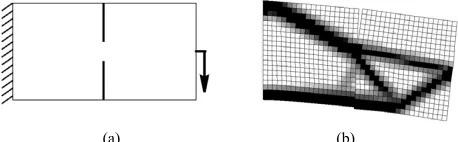
The problem of a rectangular domain was addressed by Desmorat [31]. A 2D case of a 2 × 1 rectangle with two internal contact zones, fixed at one end and loaded verti-cally at the centre of the other end is considered (see

Figure 4(a)). Figure 4(b) presents the optimization

re-sults on the coarse mesh structure with the two contact surfaces taking into account the effective contact or non- contact cases. By opposition with the result if no contact surfaces were assumed, this result shows asymmetric material distribution, an open contact zone on the upper contact surface and an effective contact zone on the lower contact surface. This observation fully agrees with the results presented by Desmorat [31].

3.2. Linked Bars

The linked bars problem, described in Figure 5(a),

con-siders the case of two 3 × 0.5 linked bars with two inter-nal contact zones, fixed at one end and loaded vertically on the other end (see [31] for more details). Figure 5(b)

presents the optimization result on the deformed struc-ture for a volume constraint of 20% and taking into ac-count the effective contact cases. Again, the results ob-tained are in agreement with the results of Desmorat [31] and, comparing with the solution without contact condi-tions, a concentration of material on the left of the link line and a different material distribution in the central part of the structure can be observed.

3.3. L-Shaped Test

The purpose of this benchmark is the verification of the behaviour in the interior corner of a L-shaped domain [32]. The geometry and boundary conditions are dis-played in Figure 6(a). A single load (upper traction of

100 MPa) pushes the structure upward while the contact condition is defined on the lateral support. The optimiza-tion result corresponding to the minimum strain energy is presented in Figure 6(b). This result is in agreement

with the results presented by Fancello [32]. It shows a concentration of material at the interior corner of the L-shaped domain and in the load surface.

(a) (b)

Figure 4. Artificial hip replacement of an uncemented prosthe-sis. A bone ingrowth is observed in the coated zones of the stem increasing the stiffness of the bone/stem interface.

(a) (b)

Figure 5. Linked bars with two contact surfaces: (a) Geometry and boundary conditions [31]; (b) optimization result for a coarse mesh and a volume constraint of 20%.

(a) (b)

Figure 6. L-shaped test with contact surface: (a) Geometry and boundary conditions [32]; (b) optimization results on the de-formed structure for a volume constraint of 40%.

3.4. Flexible Pinned Union

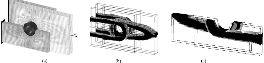
The union of three blocks with a flexible pin is modelled (see Figure 7(a)). The 3D lateral blocks are constraint in

the left edge and a horizontal load of 1000 N is applied to the central block. The lateral block dimensions are 75 × 60 × 6 mm, the central block is 90 × 60 × 12 mm and the dimensions of the cylindrical pinned are 20 × 25 mm [33]. Between the blocks, in the lateral surfaces, there are 30 mm diameter rings with 0.5 mm of thickness. All the solids are deformable but only the blocks belong to the design domain. Due to symmetry conditions, only a quarter of the geometry is modelled. The material em-ployed is steel except for the rings that are of polymeric material (elasticity modulus of 2 GPa). Frictionless con-tact conditions were considered between the pin, the rings and the blocks.

Figures 7(b) and (c) show the results obtained for a

i.e., the material that wraps the pin and the distribution is made into the constraints (the lateral block case) or into the applied load (the central block case). These results are similar to the results presented by Folgado [33] vali-dating the presented formulation.

4. VALIDATION OF THE CONTACT

INTEGRATION MODEL

The formulation presented in Section 2.3 is validated through structural problems introduced by the authors.

Progressive Contact Integration of a Compression Specimen

This problem characterizes the behaviour of a specimen subject to uniaxial compression loading. The contact surface of the specimen has a coated area, assembled by

the area of four elements that allows material integration (see Figure 8). Initially, while the material integration is

null, the behaviour of the compressed material is equal to an ordinary compressed specimen. The contour of von Mises equivalent stress in the compressed specimen and in the exterior material can be seen in Figure 8 for the

initial tine step. For this step, the tangential relative dis-placement for all nodes that belong to the material inte-gration surface is 1 × 10–7 _{< CSLIP < 1.2 × 10}–3 _{and the}

contact pressure is positive, evidencing that there is an effective contact between the two surfaces. Considering the threshold value for the relative tangential displace-ment of CSLIPLimit = 5 × 10–5 m, only the nodes that

present relative tangential displacement lower than this value will start material integration and their connector stiffness will increase. The values of CPRESSLimit and

CSHEARLimit are 0.8 and 35 MPa, respectively.

(a) (b) (c)

Figure 7. Flexible pinned union test: (a) Geometry and boundary conditions [33]; (b) optimization results on the de-formed structure for a volume constraint of 30%. Elements with relative densities inferiors of 0.1 were removed; (c) a 1 4 of the solution of the optimization domain.

By the charts of Figure 9, it can be seen that material

integration (osteointegration if the specimen is consid-ered as a bone) occurs at nodes number 33, 34 and 35 (nodes in the middle of the width of the coated surface, as represented in Figure 10). These nodes achieve full

integration at the 20th _{time step and maintain it to the end}

of the test.

In the first 6 time steps, the integration of nodes 20 and 46 (the extreme bottom nodes of the coated surface) oscillates due to the checking of the integration condi-tions. During that time, the relative tangential displace-ment decreases towards step 5 but oscillates between steps 5 and 8 (see details in CSLIP chart). The material integration conditions are successively fulfilled after step 6 and the full integration is achieved in time step 26. To note that the increasing of stiffness of the connector of nodes 33, 34 and 35 aid the decreasing of relative tan-gential displacement of theses nodes.

Nodes 21, 22 and their symmetric never attain integra-tion. The relative tangential displacements (CSLIP) chart in Figure 9 shows that, although with some oscillations,

the relative tangential displacements never decrease to a value inferior to the threshold, therefore never checking the integration conditions.

This problem characterizes well the possibility of three types of integration nodes: i) nodes that immediately start to integrate; ii) nodes whose integration depends of the integration of other nodes and iii) nodes that integration is never achieved. These occurrences take place in the osteointegration process, particularly in the bone/stem interface.

Figure 9. Time evolution of osteointegration and rela-tive tangential displacement (CSLIP) of the nodes be-longing to the coated area of Figure 10.

(a)

(b)

Figure 10. Compression specimen with an integra-tion surface: (a) Contour of the area with osteointe-gration. The value of one correspond to full integra-tion; (b) displacement contour on the deformed geometry in the final step with material integration.

5. BONE REMODELLING

PROCESS, RESULTS

5.1. Geometric Model and Domain Discretization

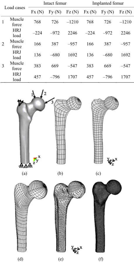
The geometry of the proximal femur and the boundary conditions used in this work are represented in figure 11a. The multiple loads applied correspond to 2.5 times of the medium weight of a human body (approximately 700 N) and can be seen in Table 1 [21]. The model is constrained

in all three directions at the nodes of the outer rim of the bottom element layer. Figure11(b) to f show the

differ-ent domain discretization used in this work. Figures 11(b), (c) and (d) show the original geometry discretized

in 1158, 5224 and 9408 hexahedral finite elements, re-spectively. Figures 11(e) and (f) present the

dense compact bone corresponds to a cellular material with relative density equal to 1 and trabecular bone has values less than 1. The elasticity modulus for dense compact bone is 20 GPa. It was also assumed a Poisson ratio of 0.3.

In the optimization process, the three load cases have the same weight and, to ensure consistency between the energy of one load and the weighted energy, it must hold that



Table 1. Load cases for the intact and implanted femurs. Intact femur Implanted femur Load cases

Fx (N) Fy (N) Fz (N) Fx (N) Fy (N) Fz (N) 1 Muscle _force 768 726 –1210 768 726 –1210

HRJ

load –224 –972 2246 –224 –972 2246 2 Muscle _force 166 387 –957 166 387 –957

HRJ

load 136 –680 1692 136 –680 1692 3 Muscle _force 383 669 –547 383 669 –547

HRJ

load 457 –796 1707 457 –796 1707

(a) (b) (c)

(d) (e) (f)

Figure 11. (a) Geometric model and boundary condi-tions of the proximal part of a femur. Discretization in (b)-(d) hexahedral and (e)-(f) tetrahedral finite ele-ments.

5.2. Initial Distribution of Material

Results of the optimization process using three values of volume constraint are given in this section. It was con-sidered different volume fractions (40%, 55% and 70%) and it was taken in account the domain discretizations represented in Figures 11(b) to (f). The optimization

process that leads to a similar result to the apparent den-sities distribution of a human femur was the process us-ing 55% volume fraction. The use of different meshes results in analogous general results, even though particular differences can be observed. Figure 12 shows the

mate-rial distribution after 100 iterations with the total volume fraction of 55%. The distribution of the relative density is interpolated from the elements to the nodes.

The results of Figure 12(a) to f show agreement

be-tween the numerical density distribution and the apparent density of the real bone. Although the shaft cavity is well represented, the densities distribution in the femoral head should be more homogeneous for the case of tetrahedral elements. This fact can be attributed to the applied load cases and the type of elements used and their importance in the numerical process.

(a) (b) (c)

(d) (e) (f)

5.3. Bone Adaptation by Stimuli Changes - Results sitivities are therefore averaged [3]. The number of times the bone is loaded has no influence in the numeric result when the limit of the bone changing is reached. In that case, a  value is found to bound the maximum bone turnover rate and the sensitivities are numerically damped (see Eq.12). Each iteration is considered a day.

After the achievement of the initial relative densities distribution, the bone adaptation to the stimuli variations is analyzed. The osteometabolic value (λ) is considered constant and equal to the value found in the initial analy-sis (λ = 1.284 N·mm–2_{). It is used the initial densities}

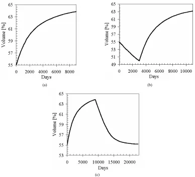
configuration as well. In the first case, and to illustrate the time dependence of the bone adaptation process, the load cases (stimulations) are multiplied by 1.5 (corre-sponding to approximately 4 times the weight of the hu-man body) during 9000 days. In the second case, the stimuli are reduced to 2/3 during 3000 days and, after-wards, increased 1.5 times. This case demonstrates bone adaptation to stimuli inversion. The third case should show the reversibility of the process. From the first case solution (Figure 13(a)), the stimulations are then kept as

the initials during more 24,000 days.

Figures 13(a), (b) and (c) show the time evolution of

the bone volume fraction for the three cases, respectively. For case 1, Figure 13(a) shows an increasing of ≈9% of

the total volume within the 9000 days. It should be notice that there are small oscillations around the volume-days curve. This case shows the influence of time and stimuli in the bone adaptation process. Figure 13(b) shows an

inversion of the bone adaptation process with the inver-sion of the load history. At first, the volume has de-creased 5% and, when the body weight has raised to four times, the volume has increased to 63%. The reversibility of the process is studied in case 3. It is known that bone tissue adaptation is an irreversible process. However, the numerical process used in this work shows a reversible process.

In the three analyses, a maximum bone turnover rate of 0.021%/day is defined [28]. A sequence of multiload cases is made in order to consider a regular day. The sen-

(a) (b)

(c)

5.4. Numerical Surgery and Remeshing

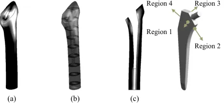
For the continuation of this work, a numerical surgery was performed in order to obtain an implanted femur. During real surgery, a part of the femoral bone is removed. First, the femoral head is removed by cutting through the femo-ral neck with a power saw. Then, special rasps are used to shape the hollow femur to the exact shape of the metal stem of the femoral component. Once the size and shape are satisfactory, the stem is inserted into the femoral ca-nal. In the uncemented variety of femoral component the stem is held in place by the tightness of the fit interfer-ence into the bone (MMG 1999). These operations were numerically conducted with the virtual femur used in the previous sections. A titanium stem similar to the Tri- lock©/Dual-Lock© of DePuy Ortopedics® was used (see Figure 14).

The pos-operative geometry of the femur was discre-

tized in 7224 hexahedral elements whose mesh is different of the original mesh (Figure 15(a)). Therefore, a

nique for transference of properties (or remeshing tech-nique) should be employed. The technique employed is based in the distance between the centre of the new ele-ment and the centre of the old eleele-ments, and can be writ-ten as (see Figure 15(b))

max 8

1 max 8

1

dist

dist

iElm iElm iElm f iElm f

iElm iElm f iElm

V x x

V



 



 

 

 

 

 







where V is the element volume and dist define the dis-tance between the centres of elements. This technique is simple and effective. Figure 15(c) shows the

transfer-ence of the relative density between the different meshes.

(a) (b) (c) (d)

Figure 14. A numerical surgery was performed in order to prepare the femur to receive a prosthesis. (a) Original femur; (b) femur after the removal of the femoral head and (b) the geometry of the titanium stem; (d) The coated and non-coated area of the titanium stem (E ≈ 115 GPa).

(a) (b) (c)

5.5. New Boundary Conditions

The boundary conditions affect significantly the results. A modification of the applied loads direction and inten-sity in the implanted femur must be considered. The hip reaction joint (HRJ) and muscles forces are modified due to geometric alterations created by each type of arthro-plasty. These alterations are due to the change of pros-thesis head position and to the changes in direction and intensity of the joint contact forces [34,35]. The different position of the stems depends not only on the geometry of stem but also on the technical procedure of the total hip arthroplasty. The prosthesis does not restore the original position of the femur head, which makes the bending moments different from the physiological origi-nal ones. Therefore, the loads and momentum equilib-rium system must be re-established. From the work of Ramos [35], considering the muscle forces unchanged, it was showed that the conditions that must be respected are the force equilibrium in the z-axis and the moments equilibrium in the x and y rotation axis [35]. The solution

of the force and moment equilibrium system of equations is listed in Table 1.

Other authors [7,9,10] also performed the correction of the muscles force when carrying out in vitro studies of different behaviour stems.

5.6. Osteointegration and Bone Remodelling Results

For the remodelling and bone ingrowth test, a tangential relative displacement threshold of CSLIPLimit = 50 μm is

used. The conditions to maintain full osteointegration are CPressLimit = 0.8 MPa and CShearLimit = 35 MPa. The

initial condition for the coated interface is set to contact with friction (coefficient of 0.3). The non-coated surfaces are considered as frictionless contact surfaces.

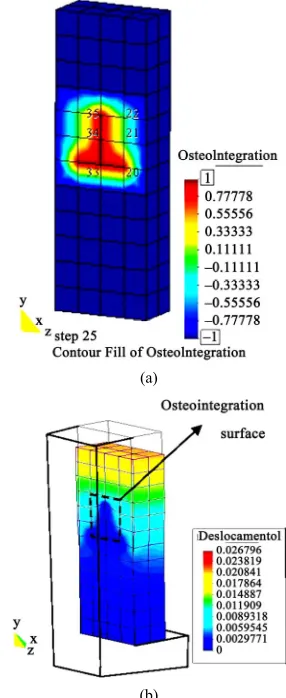
The osteointegration results (bone ingrowth), after 100 time increments, can be seen in Figure 16. The blue

re-gions indicate where the bone ingrowth does not occur - there is a separation or a relative tangential displacement greater than 50 μm. The bone ingrowth and full osteoin-tegration regions are in red. The green and orange re-gions indicate rere-gions of bone ingrowth but with no full integration.

Table 2 summarizes the full osteointegration results. It

should be noticed that there are zones with and without bone ingrowth on the coated zones. The results show higher bone osteointegration at regions 1 and 2. This can be explained by the direction of the applied load cases. However, for the time considered, bone integration was not achieved in half of the coated zone. These considera-tions corroborate clinical observaconsidera-tions [7].

(a) (b) (c) (d) (e)

Figure 16. Osteointegration results after 100 time increments: (a) Full model and scale; Details of (b) lateral left and bottom; (c) Bottom and lateral right; (d) Top and lateral right and (e) Top and lateral left coated surfaces of osteointegration.

Table 2. Surface areas of osteointegration and bone ingrowth.

Region 1 Region 2 Region 3 Region 4 Total

Total Nodes 180 144 180 144 648

Nodes with full osteointegration 40 42 5 18 105

Partial % of osteointegration 22.2% 29.2% 2.8% 12.5% 16.2%

Total osteointegration 6.2% 6.5% 0.8% 2.8% 16.2%

Figure 17 shows the bone density distribution for the

implanted proximal femur after 100 time increments. Although the overall results show the loss of bone on a proximal region of the femur, a final relative volume fraction of approximately 70% was obtained. This high volume fraction must be evaluated considering that a fraction of the original bone was removed in the numeri-cal surgery. The fraction removed (femur head) has low mean values of apparent density, therefore the remained part have higher mean volume fraction than the original bone. The region that decreased the initial global mean volume fraction, such as the intramedular cavity, is now occupied by the stem.

Comparing Figures 17 and 12, it is possible to

ob-serve the influence of the prosthesis in the density dis-tribution. First, it is observed a global redistribution of density. In Figure 12, the zone with greater density is the

diaphyseal zone, decreasing to the metaphyseal zone. Although the thickness of the cortical is thinner, in the implanted femur, there is no obvious decreasing of the volume fraction from the diaphyseal to the metaphyseal region near the region 4 of the implant. Relatively high bone density is seen in the region of front contact of the stem. The region where the head of the femur was ressected also shows high bone density. The density evolution in this region is due to the proximity to the muscle forces (the major trocanter) and to the stem. Therefore, this re-gion is subjected to high stresses. Some of the previous observations and the results of Figure 17 are similar to

the results presented in [6,7] thought the shape and size of the stem are different.

Although a lack of clinical observations subsists, it can be stated that the prediction of the model is consistent with some clinical observations of the bone relative den-sity distribution. The model presented in this work shows that osteointegration does not occur in all coated surface. This result is consistent with clinical observations [36-40] of 20% of fully osteointegration from partial coated re-covered stems. The numerical results obtain by Viceconti

et al. [12] to predict the secondary stability show higher

Region 3 Region 4

Region 1

Region 2

(a) (b) (c)

Figure 17. (a) Apparent density distribution of the implanted trabecular bone; (b) Transversals and (c) saggital longitudinal cuts of the femur’s model. The final volume fraction obtained was of approximately 70%.

values for the percentage of bonded surface, including partial or fully-bonded points. This difference can be attributed to the consideration of the bone remodelling scheme by this work, to the difference in the shape and size of the prosthesis and the coated zone. The numerical test conditions, such as the values for micromotions thresholds, were also considered different.

6. CONCLUSIONS

The remodelling scheme presented in this work is time dependent and reversible. The bone-remodelling scheme is numerically described by a time-dependent evolution-ary procedure with anisotropic material parameters. The remodelling rate equation is obtained from the structural optimization task of maximizing the stiffness subject to a biological cost associated with metabolic maintenance of bone tissue in time. Results of bone adaptation process were presented. In this process, when the stimuli are in-creased, there is a production of bone mass. When they are reduced, the bone mass is absorbed. The model pre-sented is in agreement with the generality of osteobi-ologic phenomenology. The time dependence is defined by the maximum density variation of bone. The maxi-mum value of volume variation found by [28] was used in this work.

In this work, a computational model for bone remod-elling around cementless (press-fit) stems with in growth control was also presented. The bone-prosthesis interface is modelled using a penalty contact formulation and the bone ingrowth regions are predicted using relative dis-placements and stresses criteria. During the process all the bone density, contact conditions and criteria verifica-tions are updated. Therefore, the interface stiffness can evolve to reflect the bone ingrowth phenomenon. The interface stiffness increases with the osteointegration. When reaching full osteointegration, a complete glue interface connection is achieved.

The model presented was applied to a three-dimension finite element model of an implanted femur whose initial conditions, such as the bone density, were retrieved from the previous intact bone remodelling process by means of a remeshing technique. The information about the distribution of bone ingrowth and bone density can be given by the results. The bone-remodelling scheme shows that the introduction of a femoral prosthesis compels to a new bone density distribution. Although the distribution of bone densities obtained shows small loss of bone in proximal femur, it was observed an increasing of the bone density in the neighbourhood of the prosthesis.

other authors.

7. ACKNOWLEDGEMENTS

The authors acknowledge the financial support by FCT—Fundação para a Ciência e Tecnologia—by the project SFRH/PTDC/EME-PME/ 68975/2006. The authors also thank Professor J. Folgado from ID-MEC-IST for the help in some numerical details. The article was par-tially presented at the International Conference on Engineering Opti-mization, Rio de Janeiro, Brazil, 2008.

REFERENCES

[1] Bensøe, M.P. and Sigmund, O. (2003) Topology optimi-zation—Theory, methods and applications. Springer- Verlag, BH.

[2] Huiskes, R. (2000) If bone is the answer, then what is the question? Journal of Anatomy, 197, 145-156.

doi:10.1046/j.1469-7580.2000.19720145.x

[3] Bagge, M. (2000) A model of bone adaptation as an op-timization process. Journal of Biomechanics, 33, 1349- 1357. doi:10.1016/S0021-9290(00)00124-X

[4] Fernandes, P., Rodrigues, H. and Jacobs, C. (1999) A model of bone adaptation using a global optimisation cri-terion based on the trajectorial theory of wolff. Computer Methods in Biomechanics and Biomedical Engineering, 2, 125-138. doi:10.1080/10255849908907982

[5] Fernandes, P., Guedes, J.M. and Rodrigues, H. (1999) Topology optimization of 3D linear elastic structures with a constraint on perimeter. Computers & Structures, 73, 583-594. doi:10.1016/S0045-7949(98)00312-5

[6] Fernandes, P.R., Folgado, J., Jacobs, C. and Pellegrini, V. (2002) A contact model with ingrowth control for bone remodelling around cementless stems. Journal of Biome-chanics, 35, 167-176.

doi:10.1016/S0021-9290(01)00204-4

[7] Folgado, J., Fernandes, P.R., Guedes, J.M. and Rodrigues, H. (2004) Evaluation of osteoporotic bone quality by a computational model for bone remodelling. Computers & Structures, 82, 1381-1388.

doi:10.1016/j.compstruc.2004.03.033

[8] Stolk, J., Verdonschot, N. and Huiskes, R. (2001) Hip joint and abductor-muscle forces adequately represent in vivo loading of a cemented total hip reconstruction.

Journal of Biomechanics, 34, 917-926.

doi:10.1016/S0021-9290(00)00225-6

[9] Waide, V., Cristofolini, L., Stolk, J., Verdonschot, N. and Toni, A. (2003) Experimental investigation of bone re-modeling using composite femurs. Clinical Biomechanics, 18, 523-536. doi:10.1016/S0268-0033(03)00072-X

[10] Viceconti, M., Cavalloti, G., Andrisano, A.O. and Toni, A. (1995) Discussion on the design of a hip joint simula-tor. Medical Engineering & Physics, 18, 234-240.

doi:10.1016/1350-4533(95)00026-7

[11] Viceconti, M., Muccini, R., Bernakiewicz, M., Baleani, M. and Cristofolini, L. (2000) Large-sliding contact ele-ments accurately predict levels of bone-implant micro-motion relevant to osseointegration. Journal of

Biome-chanics, 33, 1611-1618.

doi:10.1016/S0021-9290(00)00140-8

[12] Viceconti, M., Pancanti, A., Dotti, M., Traina, F., Cristo-folini, L. (2004) Effect of the initial implant fitting on the predicted secondary stability of a cementless stem.

Medical and Biological Engineering and Computing, 42, 222-229. doi:10.1007/BF02344635

[13] Viceconti, M., Ricci, S., Pancanti, A. and Cappello, A. (2004b) Numerical model to predict the long-term me-chanical stability of cementless orthopaedic implants.

Medical and Biological Engineering and Computing, 42, 747-753. doi:10.1007/BF02345207

[14] Moreo, P., Péreza, M.A., García-Aznar, J.M. and Doblaré, M. (2007) Modelling the mechanical behaviour of living bony interfaces. Computer Methods in Applied Mechan-ics and Engineering, 196, 3300-3314.

doi:10.1016/j.cma.2007.03.020

[15] Reina, E., Gómez-Benito, M.J., Garcia-Aznar, J.M., Dominguez, J. and Doblaré, M. (2007) Modelo compu- tacional de distracción ósea. Proceeding of CEMNI/ CILAMCE Conference, Sociedad Española de Métodos Numéricos en Ingeniería (SEMNI), CD-ROM paper 132, 1-10.

[16] Reina, E., Gómez-Benito, M.J., Garcia-Aznar, J.M., Dominguez, J. and Doblaré, M. (2008) Modeling distrac-tion osteogenesis: Analysis of the distracdistrac-tion rate. Bio-mechanics and Modeling in Mechanobiology, 8, 323-335. [17] Coelho, P., Fernandes, P.R., Guedes, J.M. and Rodrigues, H.C. (2008) A hierarchical model for concurrent material and topology optimization of three-dimensional structures.

Structural and Multidisciplinary Optimization, 35, 107- 115. doi:10.1007/s00158-007-0141-3

[18] Coelho, P.G., Fernandes, P.R., Rodrigues, H.C., Cardoso, J.B. and Guedes, J.M. (2009) Numerical modeling of bone tissue adaptation—A hierarchical approach for bone apparent density and trabecular structure. Journal of Biomechanics, 42, 830-837.

doi:10.1016/j.jbiomech.2009.01.020

[19] Hardy, D.C., Frayssinet, P., Guilhem, A., Lafontaine, M.A. and Delince, P.E. (1991) Bonding of hydroxyapa- tite-coated femoral prostheses. Histopathology of speci-mens from four cases. Journal of Bone & Joint Surgery, 73, 732-740.

[20] Tonino, A.J., Therin, M. and Doyle, C. (1999) Hy-droxyapatitecoated femoral stems. Histology and histo-morphometry around five components retrieved at post mortem. Journal of Bone & Joint Surgery (British Vol-ume), 81, 148-154. doi:10.1302/0301-620X.81B1.8948 [21] Fernandes, P. (1998) Optimização da Topologia de

Estruturas Tridimensionais. PhD Thesis, Instituto Supe- rior Técnico, UTL.

[22] Oliveira, J.A., Pinho-da-Cruz, J.A., Andrade-Campos, A. and Teixeira-Dias, F. (2006) Modelling the elastic be-haviour of composites materials with asymptotic expan-sion homogenisation. Proceeding of COMPTEST, 151- 152.

Computational Materials Science, 45, 1073-1080.

doi:10.1016/j.commatsci.2009.02.025

[24] Oliveira, J.A., Pinho-da-Cruz, J. and Teixeira-Dias, F. (2009) Asymptotic homogenisation in linear elasticity. Part II: Finite element procedures and multiscale applica-tions. Computational Materials Science, 45, 1081-1096.

doi:10.1016/j.commatsci.2009.01.027

[25] ABAQUS version 6.7 user manual (2006) Hibbitt. Karlsson & Sorenson. Inc.

[26] MSC.MARC (2005) Theory and User Information and User subroutines and special Routines. Msc. Software Corporation.

[27] Svanberg, K. (1987) The method of moving asymptotes – A new method for structural optimization. International Journal for Numerical Methods in Engineering, 24, 358-373. doi:10.1002/nme.1620240207

[28] Jee, W.S.S (1953) The skeletal tissues, histology: Cell & tissue biology. 5th Edition, Elsevier, Amsterdam. [29] Medical Multimedia group (1999) A Patient’s Guide to

Artificial Hip Replacement.

http://www.tri-countyortho.com/mmg/pated/joints/hip/hip _replacement.html. Accessed 15 Jan 2008

[30] Encyclo, online encyclopedia (2009)

www.ecyclo.co.uk, encyclo MMIX

[31] Desmorat, B. (2007) Structural rigidity optimization with frictionless unilateral contact. International Journal of Solids and Structures, 44, 1132-1144.

doi:10.1016/j.ijsolstr.2006.06.010

[32] Fancello, E.A. (2006) Topology optimization for mini-mum mass design considering local failure constraints and contact boundary conditions. Structural and Multid-isciplinary Optimization, 32, 229-240.

doi:10.1007/s00158-006-0019-9

[33] Folgado, J. (2004) Modelos computacionais para análise e projecto e próteses ortopédicas. PhD Thesis, IST-UTL. [34] Ramos, A. (2006) Estudo numérico e experimental de

uma nova componente Femural da prótese de Anca Cimentada. PhD Thesis, Universidade de Aveiro.

[35] Ramos, A., Fonseca, F. and Simões, J.A. (2006) Simula- tion of physiological loading in total hip replacements.

Journal of Biomechanical Engineering, 128, 579-588.

doi:10.1115/1.2205864

[36] Ramos, A. and Simões, J.A. (2006) Tetrahedral versus hexahedral finite elements in numerical modelling of the proximal femur. Medical Engineering & Physics, 28, 916-924. doi:10.1016/j.medengphy.2005.12.006

[37] Egan, J.M. and Marsden, D.C. (2001) A spring network model for the analysis of load transfer and tissue reac- tions in intramedullary fixation. Clinical Biomechanics, 16, 71-79. doi:10.1016/S0268-0033(00)00070-X [38] Sadegh, A.M., Luo, G.M. and Cowin, S.C. (1993) Bone

ingrowth: An application of the boundary element method to bone remodeling at the implant interface.

Journal of Biomechanics, 26, 167-182.

doi:10.1016/0021-9290(93)90047-I

[39] Spears, I.R., Pfleiderer, M., Schneider, E., Hille, E., Bergmannn, G. and Morlock, M.M. (2000) Interfacial conditions between a press-fit acetabulax cup and bone during daily activities: Implications for achieving bone in-growth. Journal of Biomechanics, 33, 1471-1477.

doi:10.1016/S0021-9290(00)00096-8