Numerical and experimental optimisation of a high performance heat exchanger

(1)

Numerical and experimental optimisation of a high

performance heat exchanger.

SIM, Lik F.

Available from Sheffield Hallam University Research Archive (SHURA) at:

http://shura.shu.ac.uk/20362/

This document is the author deposited version. You are advised to consult the

publisher's version if you wish to cite from it.

Published version

SIM, Lik F. (2007). Numerical and experimental optimisation of a high performance

heat exchanger. Doctoral, Sheffield Hallam University (United Kingdom)..

Copyright and re-use policy

See http://shura.shu.ac.uk/information.html

(2)

Adsetts Centre City Campus Sheffield 31 1WB

1 0 1 8 9 3 0 6 8 X

\

Sheffield Hallam University ] Learning and IT Services

r e f e r e n c e

'j Adsetts Centre City Campus

Sheffield SI 1WB

(3)

ProQuest Number: 10701008

INFORMATION TO ALL USERS

The quality of this reproduction is dependent upon the quality of the copy submitted.

In the unlikely event that the author did not send a com plete manuscript and there are missing pages, these will be noted. Also, if material had to be removed,

a note will indicate the deletion.

u

est

ProQuest 10701008

Published by ProQuest LLC(2017). Copyright of the Dissertation is held by the Author.

This work is protected against unauthorized copying under Title 17, United States C ode Microform Edition © ProQuest LLC.

ProQuest LLC.

789 East Eisenhower Parkway P.O. Box 1346

(4)

Numerical and Experimental Optimisation

of a High Performance Heat Exchanger

Lik Fang Sim

A thesis submitted in partial fulfilment o f the requirements o f Sheffield Hallam University

for degree o f Doctor o f Philosophy

(5)

This thesis is dedicated to my beloved parents and Teresa Lim, who have been giving me endless love and absolute support through life.

(6)

Abstract

The aim o f this research is to numerically and experimentally scrutinise the thermal performance o f a typical heat exchanger fitted in a domestic condensing boiler. The optimisation process considered the pins' geometry (circular pins and elliptical pins), pins' spacing, pitch distance, the pressure drop across the heat chamber and the occurrence of thermal hot spots. The first part o f the study focused on the effect o f altering the circular pins spacing and pins pitch distance o f the heat exchanger. .Computational Fluid Dynamics (CFD) is used to scrutinise the thermal performance and the air flow properties o f each model by changing these two parameters. In total, 13 circular pin models were investigated. Numerical modelling was used to analyse the performance o f each model in three-dimensional computational domain. For comparison, all models shared similar boundary conditions and maintained the same pin height o f 35 mm and pin diameter o f 8 mm. The results showed that at a given flow rate, the total heat transfer rate is more sensitive to a change in the pins spacing than a change of the pins pitch. The results also showed that an optimum spacing o f circular pins can increase the heat transfer rate by up to 10%.

The second part of the study, focused on investigating the thermal performance o f elliptical pins. Four elliptical pin setups were created to study the thermal performance and the air flow properties. In comparison with circular pins, the simulation results showed that the optimum use o f eccentricity o f elliptical pins could increase the total energy transfer by up to 23% and reduce the pressure drop by 55%.

To validate the acquired CFD results, a Thermal Wind Tunnel (TWT) was designed, built and commissioned. The experimental results showed that the numerical simulation under predicted the circular pin models’ core temperatures, but over predicted the elliptical models core temperatures. This effect is due to the default values o f the standard k - e

transport equations model used in the numerical study. Both numerical and experimental results showed that the elliptical models performed better compared to its circular pins counter parts.

The study also showed that heat exchanger optimisation can be carried out within a fixed physical geometry with the effective use o f CFD.

(7)

Acknowledgements

First o f all, I wish to thank my Director o f study Dr. Saud Ghani for his constant support, patience and encouragement throughout these years of study. Thank you for giving me the opportunity to work with you on this unique research project. It was a bumpy ride but I enjoyed every single moment o f the journey. Secondly, I would like to thank my sponsor company, Vaillant Group and Mr Steve Keeton for having me as researcher to work in parallel with the research and development group. I have enjoyed my three years working along with the research and development group.

I would like to thank Sheffield Hallam University for providing an excellent study environment and facilities for me during my research. I would also like to extend my gratitude to my second supervisor Dr. Malcolm Denman for his guidance. In no particular order, I wish to thank, Mr. Tim O' Hara, Mr. John Bickers, Mr. Brain Palmer and the technicians from the precision workshop for their assistance on setting up the thermal wind tunnel. Without their help, the experimental tests would not have been carried out successfully.

I would like to thank my parents for their understanding, belief and constant support. Sorry for not being able to stay beside you all these times.

I wish to thank my two sisters for their constant support and looking after mum and dad while I was away.

I wish to thank all my friends for their encouragement and support. I also like to express my special gratitude to my research colleague Mr. Ben Hughes for his constant support and friendship.

Finally, but by no means the least, I wish to thank a very special lady, Miss Teresa Lim for her understanding, belief, and constant support throughout my studies. Sorry for not being able to spend more time with you during this study and hopefully you will allow me to make up this time with you from this point forward.

(8)

Table of Figures

Figure 1-1: Conventional central heating system [3]...2

Figure 1-2: Modem central heating system [3]...3

Figure 1-3: Heat exchanger in condensing boiler [courtesy of Vaillant Group] ...4

Figure 1-4: Natural gas and fuel oil water vapour dew point [5]...5

Figure 1-5: Research methodology and structure... 8

Figure 2-1: Parallel flo w ... 12

Figure 2-2: Counter flow ... 12

Figure 2-3: Multiple flow s...12

Figure 2-4: (a) top view o f computational domain, (b) side view o f computational domain [11, 12]...13

Figure 2-5: Multi row plate-fin and tube heat exchanger used in Jang et al. study [1 3 ]...14

Figure 2-6: Elliptical tubes and fins used on Matos et al. studies [16]...15

Figure 2-7: Rectangular fins used on Sahin et al. studies [17 ]...16

Figure 2-8: (a) Arrangement of hexagonal pins, (b) Isometric view of hexagonal pins. [18] ...17

Figure 3-1: Algebraic methods transfer from physical domain to computational domain (a) two dimension (b) three-dimension [20]... 22

Figure 3-2: PDE mapping methods (a) physical domain, (b) computational domain [20].. 22

Figure 3-3: (a) Polygon bisected by triangles (b) DVM meshing on computational domain [21]...23

Figure 3-4: Advancing front methods (AFM) meshing construction [21]...24

Figure 3-5: FLUENT simulation structure... 35

Figure 3-6: Segregated solution method [19]... 39

Figure 3-7: Coupled solver method [19]...40

Figure 4-1: Section view o f the whole heat exchanger...43

Figure 4-2: Generic m odel... 44

Figure 4-3: Pins' spacing and pitch distance... 45

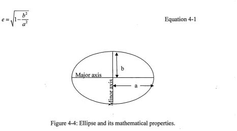
Figure 4-4: Ellipse and its mathematical properties...47

Figure 4-5: 2D and 3D cell types [24]... 49

Figure 4-6: Circular pins mesh adaption... 50

Figure 4-7: Elliptical pins mesh adaption... 50

Figure 4-8: Mesh near circular p ins...51

Figure 4-9: Mesh near elliptical pins...51

Figure 5-1: Vertical closed loop thermal wind tunnel...58

Figure 5-2: Tubular heating element § 9.53 mm x 200 mm long...60

Figure 5-3: 1/4" BSP female lock nut fitting...60

Figure 5-4: Bifurcated fan...61

Figure 5-5: Side view o f bifurcated fan ...61

Figure 5-6: Flow observation windows...62

Figure 5-7: 5 mm thick ceramic glass... 62

Figure 5-8: Specimen access window... 62

Figure 5-9: Water channel in position... 62

Figure 5-10: Industrial wire mat insulation without the protection foil... 63

Figure 5-11: Tunnel insulation with protection foil... 63

(13)

Figure 5-12: Exploded view of each section o f the TW T...65

Figure 5-13: TWT without guide vanes and screens (pressure contours)...69

Figure 5-14: Velocity magnitude o f the initial TWT design...69

Figure 5-15: TWT design with guide vanes in first comer and third com er...70

Figure 5-16: Large eddy occurred at settling zone...70

Figure 5-17: Final design o f TWT with guide vanes and wire mesh screens...71

Figure 5-18: Velocity magnitude o f the TW T...71

Figure 5-19: Wind tunnel air velocity profile...72

Figure 6-1: Benchmark CAD model... ... 76

Figure 6-2: EOS laser sintering manufacturing process [56]...77

Figure 6-3: EOSINT M270 direct metal laser sintering machine. [5 7 ]... 78

Figure 6-4: Elliptical and circular pins specimens... 80

Figure 6-5: K-type thermocouple operation principle... ...81

Figure 6-6: 2m K-type glass fibre thermocouple with miniature plug...83

Figure 6-7: 12 mm diameter flow control v alve...86

Figure 6-8: Hall effect principle [62]... 87

Figure 6-9: Fluid flow sensor...88

Figure 6-10: Frequency counter block diagram [6 3 ]... 89

Figure 6-11: Top view o f digital flow meter... 90

Figure 6-12: Front view o f digital flow meter... 90

Figure 6-13: Three phase variable fan speed controller diagram [64]...91

Figure 6-14: Single phase AC waveform rectification to DC waveform [65]...92

Figure 6-15: Three phase 1.1 kW variable speed controller...93

Figure 6-16: Fuzzy logic PID control unit...95

Figure 6-17: Inside the fuzzy logic PID control unit...96

Figure 6-18: Wind tunnel air temperature control system ... 97

Figure 6-19: Pitot tube... 98

Figure 6-20: Section view o f the pitot tube [70]...98

Figure 6-21: Absolute pressure measurement [72]... 99

Figure 6-22: Gauge pressure measurement [72]...99

Figure 6-23: Differential pressure measurement [72]... 99

Figure 6-24: Testo 521-3 flow measurement instrument... 100

Figure 6-25: Thermocouples were sealed inside the core o f the pins...101

Figure 6-26: Silicon sealant was used to fill in the hole and thermocouples position 101 Figure 6-27: Folic graphite sealant was used to secure the specimen on the water channel 102 Figure 6-28: Water flow pathway... 103

Figure 6-29: Pressure testing on specimen Ellip(8.0, 2.0) m odel ... 104

Figure 7-1: Pressure difference measurement points...107

Figure 8-1: The effects o f total energy transfer to the water side when altering the pins' spacing... 114

Figure 8-2: Benchmark model's velocity vector graph... 115

Figure 8-3: Model S I8.5 velocity vector graph... 115

Figure 8-4: Benchmark model's pins temperature contour... 116

Figure 8-5: S I8.5 model's pins temperature contour...116

Figure 8-6: The effects o f total energy transfer to the water side when altering the pins pitch distance... 117

Figure 8-7: Pressure contours on benchmark m odel... 119

Figure 8-8: Benchmark model's velocity vectors (horizontal plane)... 119

(14)

Figure 8-9: Pressure contours on S I8.5 m odel...120

Figure 8-10: Velocity vectors of model S18.5 (horizontal plane)... 120

Figure 8-11: Pressure difference o f different pins’ spacing...121

Figure 8-12: Pressure difference o f different pitch distance...121

Figure 8-13: Velocity vectors o f model PI 2.5 (horizontal plane)... 122

Figure 8-14: Temperature contours o f Benchmark-26 model... 125

Figure 8-15: Temperature contours o f model S18.5... 125

Figure 8-16: Total pressure contours of Benchmark-26 m odel...126

Figure 8-17: Velocity vectors o f Benchmark-26 model...126

Figure 8-18: Total energy transfer o f different eccentricity...127

Figure 8-19: Velocity flow vectors o f Ellip(5.5, 2.9)... 129

Figure 8-20: Model Ellip(8.0, 2.0) velocity flow vectors... 129

Figure 8-21: Model Ellip(10.0, 1.6) pins temperature contours... 130

Figure 8-22: Pressure contours o f Ellip(5.5, 2.9) model...131

Figure 8-23: Pressure distribution on Ellip(8.0, 2.0) model...132

Figure 8-24: Pressure difference o f different elliptical pins m odel... 132

Figure 8-25: Heat transfer and pressure difference performance graph... 133

Figure 9-1: Thermocouples positions in Benchmark m odel...136

Figure 9-2: Thermocouples positions in model S I8 .5 ... 137

Figure 9-3: Thermocouples positions in model Ellip(8.0, 2.0 )... 138

Figure 10-1: Benchmark model’s pins core temperature with tim e... 142

Figure 10-2: Benchmark model's water outlet temperature with tim e...142

Figure 10-3: Benchmark pins' core temperature...143

Figure 10-4: Model S18.5 pins temperatures with time...144

Figure 10-5: Model S I8.5 water outlet temperature against time...145

Figure 10-6: Model S I8.5 pins' core temperature... 146

Figure 10-7: Model Ellip(8.0,2.0) pins core temperature with tim e ...147

Figure .10-8: Ellip(8.0, 2.0) model's water outlet temperature with tim e...148

Figure 10-9: Model Ellip(8.0, 2.0) pins' core temperature... 148

Figure 10-10: Model Ellip(10,l-6) water outlet temperature against time...149

Figure 10-11: Ellip(10, 1.6) model pins' core temperature... 150

Figure B - l: Exploded view at every section o f the wind tunnel... 169

Figure B-2: Bird's eye view at the thermal wind tunnel...170

Figure B-3: Cross sectional view on test section...171

Figure B-4: Test section's dimension... 171

Figure B-5: Diffuser section's dimension... 173

Figure B-6: Third comer's dimension... 175

Figure B-7: Guide vane dimension... 176

Figure B-8: Downstream straight duct dimension... 177

Figure B-9: Fourth comer's dimension...178

Figure B-10: CAD model shows the contraction's dimension...180

Figure B -l 1: CAD model shows the dimension o f 2nd comer...183

Figure B-l 2: CAD model shows the dimension o f the expansion duct...184

Figure B-13: CAD model shows the dimension of the upstream straight duct... 185

Figure B -l 4: CAD model shows the dimension o f the 1st com er... 186

Figure B -l 5: CAD model of first comer guide vanes...187

Figure B -l 6: CAD model o f annular outlet...189

Figure B -l7: Annular Cp graph...190

Figure B -l8: Annular inlet’s CAD model... 191

(15)

[image:15.616.76.558.89.734.2]

Figure D -l: Step response using Proportional control...194 Figure D-2: Step response using proportional and integral (PI) controller... 195 Figure D-3: Step response using proportional and derivative (PD) controller... 196

(16)

Table of Tables

Table 3-1: Gambit face meshing elements options [2 4 ]...36

Table 3-2: Gambit face meshing type options [24]...36

Table 4-1.: Benchmark model’s geometric parameters...44

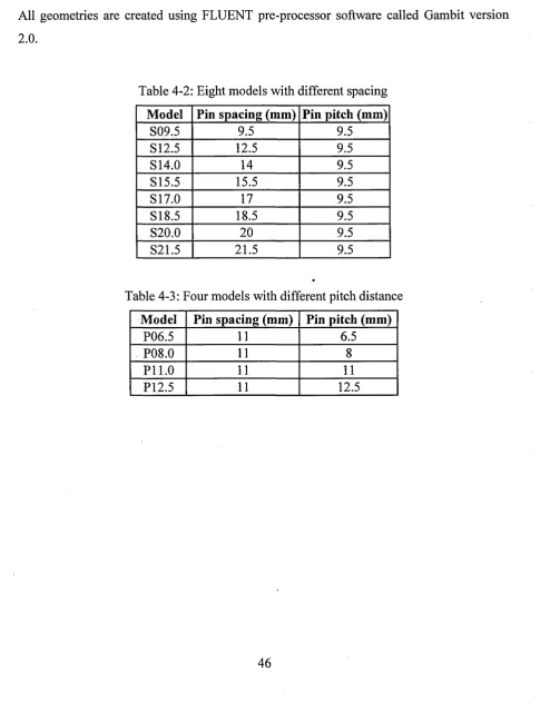
Table 4-2: Eight models with different spacing... 46

Table 4-3: Four models with different pitch distance... 46

Table 4-4: Elliptical m odels... 47

Table 4-5: Initial boundary conditions...52

Table 5-1: TWT net pressure loss calculation summary... 68

Table 5-2: Coefficient of uniformity of each design...72

Table 6-1: Material properties of DirectMetal 2 0 ... 79

Table 6-2: Pico TC-08 data logger specifications [59]... 84

Table 6-3: Equipment accuracy...104

Table 7-1 Total energy transfer o f each model with different pin spacing...108

Table 7-2: Total energy transfer o f each model with different pitch distance ... 109

Table 7-3: Elliptical pins energy transfer... 109

Table 7-4: Pressure difference at hot air channel (circular p ins)...110

Table 7-5: Total pressure difference at hot air channel (elliptical pin s)... I l l Table 8-1: Comparison between pins' spacing and number o f pins... 124

Table 9-1: Experimental and numerical simulation results o f the Benchmark m odel 135 Table 9-2: Experimental and numerical simulation results o f model S18.5... 136

Table 9-3: Experimental and numerical simulation results o f Ellip(8.0, 2.0) m odel 137 Table 9-4: Experimental and numerical simulation results o f Ellip(10.0, 1.6) model 139 Table 10-1: Total energy transfer o f each m odel...151

Table 10-2: Numerical simulation results o f Benchmark model when CM = 0.085... 152

Table B -l: Pressure loss coefficient for diffuser...174

Table B-2: Pressure loss coefficient for elbow ...175

Table B-3: 90 degree bend guide vane pressure loss coefficient table ...187

(17)

Nomenclature

u x - momentum, (kg-m/s) V y - momentum, (kg-m/s)

w z - momentum, (kg-m/s)

Sm Mass added to the continuous phase from the dispersed second phase and any user defined sources, (kg)

P Static pressure, (Pa)

keff Effective conductivity, (W/ m-K)

J J Diffusion flux, (mol/ m s)

sh

Heat o f chemical reaction and other volumetric heat sources from user, (W)

h

Enthalpy, (J/kg)

Yj Mass fraction o f species j

I

Unit tensor

k Turbulence kinetic energy, (m2/s2)

G k Generation of turbulence kinetic energy due to the mean velocity gradients

Gb Generation o f turbulence kinetic energy due to buoyancy

Ym Fluctuating dilation in compressible turbulence to the overall dissipation rate

sk

User defined source term for turbulence kinetic energy, (m2/s2)

S£ User defined source term for turbulence dissipation rate, (m2/s3) Dh Hydraulic diameter, (m)

m Mass to be heated, (kg)

cp

Specific heat capacity o f the fluid, (kJ/kg-K)

AT Temperature difference, (K)

t Temperature rise time, (hrs)

U Overall heat transfer coefficient, (W/ m-K) A Wind tunnel surface area, (m2)

BSP British Standard Pipe Re Reynolds Number

P0 Pressure head at fan outlet, (Pa) Vo Outlet velocity, (m/s)

vi Inlet velocity, (m/s)

Pi Pressure head at fan inlet, (Pa)

K-i Sum of total pressure head loss between fan outlet and inlet, (Pa)

Q

Volume flow rate, (m /s)

Pa Fan power, (W)

cu

Coefficient o f uniformity

Vmax Maximum air velocity, (m/s)

Pm in Minimum air velocity, (m/s) Vavg Average air velocity, (m/s) V Voltage, (V)

Th Measured temperature, (°C) EMF Electro Magnetic Field

VH Hall effect voltage, (V)

(18)

I Current, (A)

B Magnetic field, (N s)

d Depth o f the plate, (m)

e Electron charge, (m kg s)

n Bulk density o f carrier electrons, (m'3) f Frequency, (Hz)

n Number of cycles o f the repetitive signal

t Time, (s)

P Pulses per minute

K Pulses per litre

RPM Revolution Per Minute

/ Supplied frequency to the motor, (Hz)

P Number o f motor poles Pout Proportional term

K P Proportional gain

e Measured error

t

Process time, (s)

^out Integral term

Kt Integral gain Dout Derivative term Kd Derivative gain

Pt Measured total pressure , (Pa) Ps Measured static pressure, (Pa)

V Defined velocity, (m/s) AP Pressure difference, (Pa)

PupstreamUpstream pressure, (Pa)

P^nstrcan,Downstream pressure, (Pa)

Greek symbol

v Fluid flow velocity, (m/s)

p Local density, (kg/m3)

2 2

p g Gravitational body force, (kg/ m s ) r Stress tensor, (N/m )

p. Molecular viscosity, (Pa s) ₀_^ s Turbulence dissipation rate, (m /s )

<Jk Turbulent Prandtl number for turbulence kinetic energy

c £ Turbulent Prandtl number for energy dissipation rate t Time in the past contributing in the integral response, (s)

(19)

Chapter 1

Introduction

Research shows that the earth’s surface temperature increased by 0.6 ±0.2°C during the 20

century. This caused the global mean sea level to increase at an average annual rate o f 1 to

2 mm [1]. By the year 2010, the United Kingdom's (UK) Government pledges to reduce the

carbon emissions from British homes by 20% compared with the average emission rate of

the year 1990 [2]. Domestic home boilers have direct impact on the domestic emissions

target, thus it is important to design more efficient and intelligent boilers.

Overview

The majority of UK homes utilise gas fired central heating to supply hot water and heating

around the house. As depicted in Figure 1-1, a conventional central heating system consists

of the following:

1. Conventional boiler

2. Timer

3. Room thermostat

4. Cold water storage tank

5. Cylinder

6. Expansion tank/ vessel

7. Radiators

(20)

Cold water storage tank

(4)

Radiator

Room H oorn

1 h e r m us Lit

thermostat

ram mer

Timer (2)

Expansion tank/ vessel

(6)

Cylinder

Conventional

boiler (1)

Figure 1-1: Conventional central heating system [3]

Cold water from the storage tank or mains supply, replenishes the cylinder when water has been released from the cylinder. A conventional boiler is used to raise the water temperature inside the cylinder for household usage and home heating. A pump is used to circulate the water from the cylinder to the radiators. As illustrated, a conventional central heating system utilises more heating space in the house. If the cylinder does run out of hot water it will usually take 25 to 30 minutes for the water to recover. Another disadvantage of a traditional boiler is that a large quantity of excessive heat is wasted when there is no demand for hot water.

Figure 1-2 shows a modem condensing boiler supply hot water and heating around the house without using any cylinder or cold water tank. Unlike conventional central heating, hot water is supplied on demand basis. A modem condensing boiler converts more than 90% of fuel into heat, compared to 78% using a conventional boiler. Any conventional boiler over 15 years old is considered inefficient because it only converts 50% of fuel into heat [4].

2

(21)

Radiator

Condensing boiler

Figure 1-2: Modem central heating system [3]

A high efficiency condensing boiler bums natural gas in a heat chamber surrounded by a water jacket as illustrated in Figure 1-3. This unit is known as the heat exchanger. The heat exchanger plays a vital role within the boiler, as it is where the energy conversion and exchange would occur. The heat exchanger is a device in which energy is transferred from one fluid to another across a solid surface. The solid surface usually contains large quantities of pins to increase the total surface area available for heat exchanging process. Water channels or waterways externally encase the heat chamber to pick up the generated heat and transfer it to the water side.

(22)

Hot gas inlet

Water outlet

Water inlet

Hot gas outlet

Figure 1-3: Heat exchanger in condensing boiler [courtesy of Vaillant Group]

The principle behind a condensing boiler is to recover as much heat as possible from the gas and further absorb the sensible heat from the condensate water before rejecting it to the

atmosphere. In natural gas (methane CH4), the simplified combustion equation can be

written as:

CH4 + 2 02 + 7.2 N2 -> 2 H20 + C 02 + 7.2N2 + 30 kW of heat Equation 1-1

Fuel: CH4 = 16 kg/k mol

Air: 2 02 + 7.2 N2 = 274.6 kg/k mol

Products: 2 H20 + C 02 + 7.2N2 = 290.6 kg/k mol

(23)

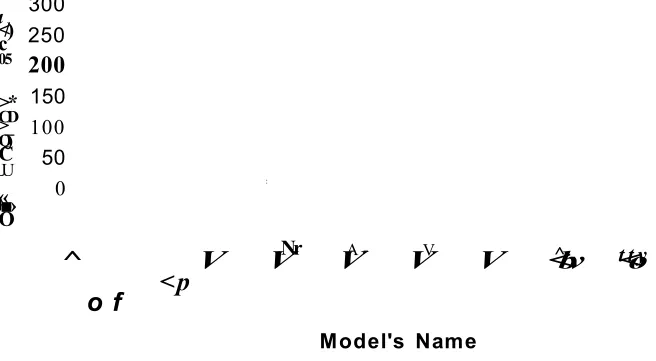
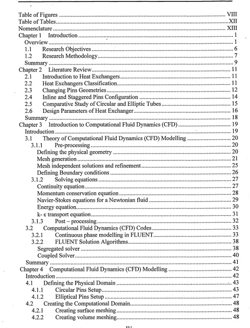
If the wall temperatures at the heat chamber fall below the water vapour dew point, condensation will occur. Figure 1-4 illustrates that the water vapour dew point is

approximately 57 °C. Currently, for natural gas (95% CH4) condensing boilers exiting

temperature is between 50°C to 60°C compared with 120 to 180 °C in current non condensing boilers. Figure 1-4 also shows that the lower the sensible heat from the water vapour that is drawn out, the lower the carbon dioxide content released to the atmosphere.

60

Natuial gas (95% CH4) 57

55

EL

-ue

50

45

40

O

+-» .£ 35

oa o

-O 30

3

oa

5 25 *—

o

to

5

1 2 3 4 5 6 7 8 9 10 11 12 13 14 15

C02 content [vol. %]

Figure 1-4: Natural gas and fuel oil water vapour dew point [5]

[image:23.615.141.496.160.553.2]

(24)

1.1 Research Objectives

The aim o f this research was to numerically and experimentally scrutinise the thermal

performance o f a typical heat exchanger fitted in a domestic condensing boiler. The

optimisation process took into account the pins’ geometry (circular and elliptical pins),

pins' spacing, pins pitch, the pressure drop across the heat chamber and the occurrence o f

thermal hot spots.

The main objectives of this research on current heat exchangers are to:

1. Scrutinise the sensitivity o f the geometrical performance o f circular pins

2. Scrutinise the sensitivity of the geometrical performance o f elliptical pins

3. Design, build and commission a thermal wind tunnel

4. Validate numerical simulation results against experimental results

5. Improve the thermal efficiency o f a current heat exchanger taken as a benchmark

without physically altering the size, weight and volume o f the unit.

The first stage o f this research investigates the thermal and fluid flow performance o f fixed

diameter circular pins. In total 13 models with different pins' spacing or pitch distance were

investigated. The second stage o f the research evaluates the performance o f the

conventional circular pins’ thermal performance against elliptical pins.

The third stage of the research introduces the experimental equipment used. A thermal wind

tunnel was designed and enhanced using Computational Fluid Dynamics (CFD) tool. The thermal wind tunnel was then built and commissioned to experimentally validate the

acquired numerical results. Direct Metal Laser-Sintering (DMLS) technology was used to

build the pin models out o f copper alloy which was tested on the thermal wind tunnel.

Experimental data acquired from the thermal wind tunnel were then used to validate the

numerical results.

(25)

1.2 Research Methodology

Both computational and experimental methods were used to study the thermal performance

o f the heat exchanger. Figure 1-5 illustrates the methodology and the logical thread

structure used in this research. The first stage o f the study focuses on the thermal and fluid

flow performance of 4 x 4 staggered circular pins, with different spacing and pitch distance

in a fixed channel. The numerical studies were conducted using commercially available

CFD code, FLUENT 6.2. A model taken from a current market production heat exchanger

was used as a benchmark design. From this model, several different pins configuration

models with the same boundary conditions were then compared on the basis o f maximising

the total energy transfer from the pins to the water and reduce the pressure loss within the

hot air channel.

The second stage o f the research focused on the thermal and fluid flow performance o f 4 x

4 staggered elliptical pins with different eccentricities. All elliptical models have the same

material volume as their circular pins counterparts.

The third stage o f this research shows the design, building and commissioning of a thermal

wind tunnel. Due the specific application requirements, the thermal wind tunnel had to be

custom made to suit the experimental tests. The initial design focuses on the flow quality

within the thermal wind tunnel. Furthermore, the thermal wind tunnel design enhancement

was carried out using CFD code, FLUENT 6.2. The specimens are then experimentally

assessed in the thermal wind tunnel. Experimental results obtained from the thermal wind

tunnel gave the thermal distribution o f the pins' core temperature and thermal performance

of each model. The experiment data was used to validate the numerical models.

The acquired data for numerical validation provides confidence in concluding the

justification.

(26)

CFD Studies Experimental Study

CO

<+H

co

C

w

3

a)

R

JtJ

.a

-3

£

§

.3

+-*

O

(27)

Summary

This thesis is divided into 11 chapters. Each chapter covers a topic deemed necessary for

this research. A summary of each chapter is listed below:

Chapter 1 provides an introduction o f present domestic heating system and

conventional heating system. This chapter also summarises the research objectives and

methodology used in this research.

Chapter 2 presents previous related publications that have been published in different

journals. Topics selected ranging from heat exchanger classification to the design

parameters o f heat exchanger.

Chapter 3 introduces CFD and its solution algorithms as a design tool used in this research. The chapter covers the theory o f CFD and the modelling methods employed.

Chapter 4 summarises the numerical modelling methods employed in this research. The

chapter covers the topics from computational meshing to solution convergence.

Chapter 5 introduces the design criteria o f the thermal wind tunnel. A summary o f the

thermal wind tunnel numerical calculations is given in the chapter. A further design

optimisation o f the thermal wind tunnel is also discussed in the chapter.

Chapter 6 introduces the manufacturing process used to create the generic models

namely, Direct Metal Laser Sintering (DMLS) technology. The chapter also introduces

the instruments used throughout the experimental tests. Specimen preparation and water

loop pressure testing were also described in the chapter.

Chapter 7 summarises the numerical simulation results.

Chapter 8 evaluation and analysis o f the flow pattern and heat transfer results acquired

from computer simulation is given.

(28)

Chapter 9 summarises the flows conditions and data acquired from the experimental tests.

Chapter 10 evaluates and validates the numerical results using the data acquired from

the experimental tests.

Chapter 11 concludes this research and presents future work that could be carried out.

(29)

Chapter 2

Literature Review

A literature review has been carried out in this study to gather the previous related work on

heat exchanger design and optimisation.

2.1 Introduction to Heat Exchangers

A heat exchanger is a device, which is used to transfer thermal energy from hotter fluid to a

colder fluid [6]. Heat exchangers can be operated in three different ways and they are

recuperation, regeneration and direct contact [7]. The most common heat exchanger is the

recuperation heat exchanger, which transfers heat between two fluids separated from each

other by a wall or a partition. Regeneration heat exchangers consist o f either a moving

wheel or fixed matrix. They are often found in gas turbines, where they are used to preheat

combustion gases by the exhaust stream. Direct contact heat exchangers are commonly

found in the metal sheet drawing industry. For example, cooling metal sheet by water

droplets as it leaves a rolling press and in cooling towers where water droplets are cooled

by an up draught o f air [7].

2.2 Heat Exchangers Classification

Heat exchangers can be classified according to the flow arrangement. The flow

arrangements can be parallel flow, counter flow, cross flow or multiple passes. In parallel

flow heat exchangers, both fluids flow in from the same direction into the heat exchanger

[8]. Conversely with counter-flow, two fluids at different temperature enter the heat

exchanger at opposite ends and heat is transferred continuously from the hotter fluid to the

colder fluid along the length of the heat exchanger [6]. Both flow characteristics can be

found in Figure 2-1 and Figure 2-2. When two working fluids flow paths are perpendicular

then the process is known as cross flow. In complex heat exchangers, multiple passes are

used to increase the heat transfer rate because fluid transverse the heat exchanger several

times before exiting. The operating principle o f multiple passes can be found in Figure 2-3.

(30)

Hot fluid

C old fluid

7

Length or area

S h ell

7

Tube

Length or area Hot fluid

7

Cold fluid

Length qr area

Figure 2-1: Parallel flow Figure 2-2: Counter flow Figure 2-3: Multiple flows

[

6

]

[

6

]

[

6

]

2.3 Changing Pins Geometries

Research [9 -1 8 ] has been carried out to discover the most efficient pins geometry for each

individual heating application. The common pins geometry used in the heating industry

ranges from convectional circular pins to hexagonal pins. This research conducted a

thorough review on different pins geometries. Behnia et al. [9] used computational fluid

dynamics software to analyse the thermal performance of circular, square, elliptical and

parallel plate fins heat sinks. The authors also used both inline and staggered arrays on each

geometry studied. All geometries in the study were compared based on air velocity between

0.5 to 5 m/s and equal wetted area o f the fins per unit base area. The authors concluded that

at a given pressure drop, the staggered plate and staggered elliptical heat sink performed

better than other geometries. The authors concluded that at lower values o f pressure drop

and pumping power, elliptical fins work best.

Christopher et al. [10] used an experimental approach to study elliptical pins, cross cut pins

and straight fins. The authors conducted a series of tests on different air velocities ranging

from 0.5 m/s to 1 m/s in a wind tunnel. Their report showed that the heat transfer on

elliptical pins is much better than cross cut pins and straight fins. In open or confined flow,

straight fin showed less effect on the pressure drop.

Kyoungwoo et al. [11] studied the flow and heat transfer o f staggered cone shape pins

geometry (spacing and pitch) and its shape (upper and lower diameter o f the cone pin) in

two-dimensional form. The flow and thermal characteristics of the reference staggered cone

pins were first analysed using Finite Volume Method (FVM). Later, a Sequential Linear

(31)

Programming (SLP) algorithm method was used to optimise the design. They concluded

that the most dominant factor for pressure drop and heat transfer rate is the lower diameter

D2, as depicted in Figure 2-4, o f the cone pin and the pins’ spacing. The research work

showed that increasing the pins’ spacing is more efficient than altering the pins pitch

distance. The authors also concluded that the total heat transfer is more sensitive on the

change of the heat exchanger area than the temperature gradient.

Similar study, but in three-dimensional form was found using four dimensionless geometric

parameters to study cone pins in a fixed channel by Lee et al. [12]. Four dimensionless

geometric parameters of the pins were selected as an important design variables in the

study, namely the pins' spacing (L), pin volume (V), the angle (p) and pitch distance (G) as

depicted in Figure 2-4.

outlet

periodic

x

{ }

inlet

( f l) T o p '

MMZX-ji'n'm ciric plane

z

x

(b) ITont 1, icv.

Figure 2-4: (a) top view of computational domain, (b) side view o f computational domain

[11, 12]

The authors affirmed that when increasing the cone spacing, the heat transfer rate increases

and the pressure drop reduces. The study also showed that changing pitch distance does not

give any significant improvements on heat transfer and pressure drop because most o f the

flow passes through both sides of the channel as in the case o f small pins’ spacing. The

authors also carried out an optimisation process to minimise a global objective function

(32)

consisting o f the correlation between the Nusselt number and the friction factor. The

authors concluded that the optimum geometric parameters obtained can be applied to

Reynolds number ranging between 500 and 1500. The most influencing parameters to the

thermal and flow performance in the highest sensitivity order is pins' spacing, volume, cone angle and pitch distance.

2.4 Inline and Staggered Pins Configuration

The most common pin configurations can be inline or staggered configurations. Some

research has been carried out to study the effectiveness o f both configurations. Previous

study was found from Jang et al. [13] who used computational and experimental methods

to study the fluid flow and heat transfer o f a multi row plate-fin and tube heat exchanger.

The study focused on two different arrangements; inline and staggered pin configuration as

illustrated in Figure 2-5.

Tube

Fin G*$ —

-Fin

Gas

(b) In-lined arrangement

(a) Staggered arrangement

Figure 2-5: Multi row plate-fin and tube heat exchanger used in Jang et al. study [13]

The authors found that the average heat transfer coefficient of the staggered arrangement is

15% to 27% higher than the inline arrangement but it suffered from high-pressure drop.

The pressure drop was 20% to 25% higher than the inline arrangement. In the staggered array, the authors detected a small recirculation zone behind each tube, due to repeated

blockage of the staggered tube bank. On the inline array, the flow separates at the rear

portion o f a tube and reattaches at the front portion o f the following tube to form a larger

stationary recirculation region between the two adjacent tubes, causing a stagnant zone.

This work showed that the staggered array outperformed the inline array.

(33)

2.5 Comparative Study of Circular and Elliptic Tubes

More direct comparison studies between circular and elliptic tubes were found through out

this review. Rocha et al. [14] analysed the heat transfer performance of one and two rows

of circular and elliptical tubes. Throughout their studies, elliptical configuration showed better efficiency than a circular counterpart. The maximum relative efficiency gain on

elliptical tube was 18% on eccentricity of 0.5. A further study from Matos et al. [15] was

found, which used numerical approach to investigate a two-dimensional heat transfer performance of circular and elliptic tube heat exchangers. The study used Finite Element Method (FEM) to define the model’s fluid flow and heat transfer. The study focused on the optimal spacing of staggered circular and elliptical tubes in a fixed volume. The circular and elliptical arrangements with the same flow obstruction cross-sectional area were compared. They concluded that elliptical arrangement heat transfer was about 13% more than the circular counter parts. The authors also stated that the flatter the ellipses are, the higher the overall heat transfer will be.

Recently, Matos et al. [16] presented another study on circular and elliptical tubes fins’

thermal performance. The study focused on three-dimensional numerical and experimental geometric optimisation. The optimisation parameters were tube to tube spacing, eccentricity and fin to fin spacing as shown in Figure 2-6.

(t+6)/2

flow

tube /

Figure 2-6: Elliptical tubes and fins used on Matos et al. studies [16]

(34)

The investigations were based on laminar regime for Re = 100 and 125. The study concluded that the three-dimensional elliptical model has a relative heat transfer gain up to 19% in comparison with circular tubes. The results also showed that fin’s temperature on elliptical tubes is more uniform than the one on circular tubes.

2.6 Design Parameters of Heat Exchanger

Recently, Sahin et al [17] studied the heat transfer and pressure drop characteristics of

rectangular fins by changing the fins width (b), stream wise distance between slices (e),

span wise distance slices (/'), angle of attack (a), heights of the fins (/ik), stream wise

distance between fins (c), span wise distance between fins (a) and flow velocity as shown in

Figure 2-7.

f s

o r *

Figure 2-7: Rectangular fins

(b)

sd on Sahin et al. studies [17]

The authors used experimental techniques to analyse the identified design factors. According to their argument, the most influential parameters on heat transfer rate were identified as follows: fin height, fluid velocity, stream-wise distance between slices, span wide distance between slices, fin width, span wise distance between fins, angle of attack and stream wise distance between fins. The results also showed that when increasing the fin height, the heat transfer surface increases but the heat transfer coefficient decreases. As for the most influencing pressure drop factors were: angle of attack, fin width, fluid velocity

(35)

and span wise distance between slices where, the rest of the parameters does not show any significant changes in friction factor. Overall, the optimisation priorities among all these factors were found to be the fin width, angle of attack, fin height and span wise distance between fins.

A study carried out by Yakut et al. [18] examined the design parameters of hexagonal pins

heat exchangers. As depicted in Figure 2-8, the effect of the height, widths of the hexagonal pins, streamwise and spanwise distance between pins and flow velocity on thermal resistance and pressure drop were investigated. The study concluded that the most important parameters affecting the heat resistance and pressure drop are pin height, pin width, spanwise distance between pins and streamwise distance between pin.

flow

(a) (b)

Figure 2-8: (a) Arrangement of hexagonal pins, (b) Isometric view of hexagonal pins. [18]

(36)

Summary

After reviewing previous related published works, it is evident that most previous studies

only focused on the effects o f different pins geometries, for example square pins or

elliptical pins. Although, Sahin et al. [17] studied the effects o f the fin stream-wise and

spam-wise distance, rectangular fins were used instead o f circular pins in their study.

Furthermore, Matos et a l [16] investigations were very similar to this research but the

authors only focused on laminar flow scenario. To the author’s knowledge no publication

was found, studying heat transfer from the solid phase to fluid phase.

Using Kwan-Soo Lee et al. [6] publication as a reference material, this research will focus

more on pins' spacing to improve the heat exchanger performance rather than focusing on

the pins pitch. This research differs from Kwan-Soo Lee et al. [6] as they only focused on

laminar flow on cone pins and further more, the authors did not utilise any coolant or water

in their study.

Consequently, this research will focus on:

• Air flow on circular and elliptical pins at Reynolds number o f 1.7 x 104.

• Using two different fluids on test models. Air temperature o f 200°C and cold water

of 17°C as the heat carrier.

(37)

Chapter 3

Introduction to Computational Fluid

Dynamics (CFD)

Introduction

During the earlier twentieth century, physicists and scientists used experimental and

theoretical methods to study fluid dynamics. However, the advancement of high speed

computing power and mathematical modelling introduced an important new approach in

fluid dynamics known as Computational Fluid Dynamics (CFD). CFD is a scientific tool of

predicting fluid flow, heat transfer, mass transfer, phase change, chemical reaction,

mechanical movement, stress or deformation o f related solid structure and related

phenomena by solving the mathematical equations that govern processes using a numerical

algorithm on a computer [19]. CFD is an important tool in modem research. Numerous

fluid dynamics problems have been studied and optimised using computational studies

before any experimental work was carried out. Sometimes CFD simulation permits the

investigation to be carried out, where controlled experiments are difficult to achieve. For

example, temperature at a particular point inside the heat chamber o f the heat exchanger.

CFD simulations are most useful in predicting the trends o f how shape changes affect the

flow field and heat transfer o f the system. The ultimate advantage o f the CFD over

experiment is practically the unlimited level o f detail o f results it has.

This chapter presents a brief introduction o f the theories behind CFD and modelling steps

using CFD codes. Only relevant numerical models for this study will be presented here.

The numerical simulation steps described in this study are based on FLUENT 6.2 CFD

code.

(38)

3.1 Theory of Computational Fluid Dynamics (CFD) Modelling

There are several commercially available CFD codes on today’s market. The most

commonly used CFD codes are FLUENT, STAR-CD, CFX and CFD-FASTRAN. CFD

simulations are summarised in three main steps:

1. Pre-processing

2. Solving equations

3. Post - processing

Each step will be discussed briefly within this chapter.

3.1.1 Pre-processing

Pre-processing can be carried out using different Computer Aided Design (CAD) or

Computer Aided Engineering (CAE) package for example Pro/Engineer Wildfire,

SolidWorks or Gambit. The activities involved in pre-processing are:

1. Defining the physical geometry o f the region o f interest

2. Mesh generation

3. Mesh independent solutions and refinement

4. Define appropriate boundary conditions at boundaries

Defining the physical geomet

ry

Before any CFD models can be solved, the geometry o f the interested system must be

defined. All CFD codes require a geometrical model as a starting point. A geometrical

model o f a system is also known as the physical domain. A geometrical model can be

created in any CAD package that is available on the market.

(39)

Mesh gene

ra

tion

Mesh generation is one o f the most important and most time consuming processes in CFD

simulation. It is also known as grid generation. Mesh generation is the approximation of the

continuous surfaces o f the object and the continuous physical volume through a set o f

discrete x, y, z coordinates. The quality o f mesh plays a significant role on the results

accuracy and solution stability. The attributes associated with mesh quality including node

point distribution, smoothness and skewness o f mesh. An improper mesh can affect the

physics o f the flow simulated, solution stability and computing time. There are two types o f

mesh generation schemes to represent the model in computational domain. They are:

1. Structured mesh

2. Unstructured mesh.

Structure mesh can be divided into two types:

1. Algebraic methods

2. Partial Differential Equation (PDE) mapping methods.

As shown in Figure 3-1, in algebraic methods, geometric data o f the Cartesian coordinates

in the interior o f a domain are generated from the values specified at the boundaries

through interpolations or specific functions o f the curvilinear coordinates [20]. PDE

mapping methods are more complicated than algebraic methods but provide smoother mesh

generation. PDE mapping methods use partial differential equations to transfer physical

domain to computational domain. The partial differential equations can be elliptic,

hyperbolic, or parabolic. The mesh generated using PDE mapping methods is shown in Figure 3-2.

(40)

4

1

Physical domain

i

(0,1) (1,1). 3

2 _

(0,0) (1,0)

Transformed computational domain

(a)

z

(0,1,1) (1,1,1)

✓ ✓

IX

(0,0,0) (1,0,0) /

/ /

^ (1,1,0)

(b)

Figure 3-1: Algebraic methods transfer from physical domain to computational domain (a)

two dimension (b) three-dimension [20]

Streamlines or x-coordinates Velocity potential

or y-coordinates

(a)

Figure 3-2: PDE mapping methods (a) physical domain, (b) computational domain [20].

Unstructured mesh offers more flexibility on complex and irregular geometry. Structured

mesh is restricted to where physical domain can be transformed into computational domain

through one to one mapping. There are two major unstructured mesh generation methods:

(a) Delaunary-Voroni Methods (DVM) and (b) Advancing Front Methods (AFM) for

triangles in two dimensional and tetrahedral in three dimensional. In DVM a two

(41)

dimensional domain may be triangulated as shown in Figure 3-3. Each side line o f the triangles can be bisected in a perpendicular direction such that these three bisectors join a

point within the triangle forming a polygon surrounding the vertex o f each triangle. DVM

prefer triangle close to an equilateral triangle than distorted triangular shapes.

(a) (b)

Figure 3-3: (a) Polygon bisected by triangles (b) DVM meshing on computational domain

[

21

]

AFM use internal nodal formation and triangulation to generate mesh. As shown in Figure

3-4, simple domains with six nodes are used as initial active front face. Node 7 is created to

form a triangular 1-2-7 and then side 1-2 is deleted so that now two new front faces 1-7 and

2-7 are created. The process continues until all front faces are deleted as shown in Figure

3-4. The deleted sides then represent the generated mesh [21]. This type o f mesh generation

method is more controllable on the node spacing especially when coarse and fine meshes

are together. This type o f meshing can also cause cells to be skewed for example cells

collapse on other cells. In some CFD codes, the quality o f the generated mesh as a function

of its skewness can be shown after meshing.

(42)

4(1 0, 2)

(a) Given domain

6

(c) Choose new node (7), delete side (1-2), new active fronts (1-7,2-7)

(e) Delete sides (3-8,3-4), new active front (8-4)

1

2

(b) Background boundary nodes (initial fronts)

6

(d) Choose new node (8), delete side (2-3), new active fronts (2-8,3-8)

(f) Delete sides (4-8,4-5), new active front (5-8)

1

(g) Delete side (5-6), new active fronts (5-7, 6-7)

1

(h)Delete sides (6-7,6-1,1-7), no new active front

6

1

(i) Delete sides (2-7,2-8), new active front (7-8) (j) Delete sides (7-8,7-5, 8-5), no new active front

Figure 3-4: Advancing front methods (AFM) meshing construction [21]

(43)

Mesh independent solutions and

r

efinement

The aim o f CFD simulation is to obtain acceptable results while minimising the

requirements o f computing power. In general, the larger the number o f cells used in a

model the better the representation o f the physical domain and hence the better the

accuracy. In many cases, CFD users want to achieve accuracy and efficiency at the same

time. Thus, mesh independent methods are utilised to assess both accuracy and efficiency at

the same time. Depending on which mesh generation scheme used, a suitable mesh

independent method could be selected. Structured mesh scheme can use (1) control

function methods or (2) variation function approach. Both methods use redistribution

method to move the grid points in accordance with the weight or control functions on the

gradients of the variable. More details o f these two methods can be found in reference [22].

Due to flexibility on node spacing, unstructured mesh scheme allows users to adopt more

than two different mesh independent methods. The mesh independent methods used on

unstructured method are:

1. Mesh refinement methods (h - methods)

2. Mesh movement methods (r - methods)

3. Mesh enrichment methods (p- methods)

4. Combined mesh refinements and movements (hr - methods)

5. Combined mesh refinements and enrichments (hp - methods) [22].

This Chapter will focus on unstructured mesh independent methods because it is adopted in

this research. Mesh refinement methods (h - methods) is to refine the mesh based on an

error indicator. An error indicator is the solution gradient variables for example density,

pressure or temperature. It indicates how fast the error changes as the refinement changes.

This refinement is carried out until the solution reaches the user specified tolerance. Mesh

movement methods (r - methods) is slightly different compared with mesh refinement

methods (h - methods) because instead o f mesh refinement, grid point can be moved

around to more sensitive areas. This method can reduce the number o f cells, but also

increase the results accuracy. This method also use error indicator to reach user specified

tolerance. Mesh enrichment methods (p- methods) is different from the above methods.

(44)

Geometry is assigned with a fixed mesh and the solutions are expected to improve by running higher polynomials or higher order functions. If the solution fails to reach the user

specified tolerance, the relating order must be raised. Combined mesh refinements and

movements (hr - methods) is the most flexible mesh improvement method. It refines and

moves around the grid points to more sensitive areas to achieve better accuracy in

simulation results. If a simulation model is involved in a shock wave interacting with

turbulent boundary layers, combined mesh refinements and enrichments (hp - methods) is

not recommended [22]. This method begins with lower polynomial or order until h

-methods reach to a certain level i.e. shock discontinue, then followed by p - enrichment.

Defining Bounda

ry con

ditions

Numerical and experimental optimisation of a high performance heat exchanger

Numerical and experimental optimisation of a high

Published version

Adsetts Centre City Campus Sheffield 31 1WB

Numerical and Experimental Optimisation

A thesis submitted in partial fulfilment o f the requirements o f Sheffield Hallam University

Abstract

Acknowledgements

CONTENTS

Table o f Figures... ... VIII Table o f Tables... XII Nomenclature...XIII

2.6 Design Parameters o f Heat Exchanger...16

Momentum conservation equation... 28

Introduction... 42

Chapter 5 Thermal Wind Tunnel Design...56

5.1.7 Tunnel insulation... 63

6.4.1 K-type thermocouples... 81

Fuzzy logic control...94

7.2 CFD Pressure Difference Results... 110

8.5 Elliptical Pins - Pressure Difference...131

Introduction... 140

Appendix B Thermal Wind Tunnel (TWT) Design and Calculations...168

B.14 First com er... 186

Appendix E Wind Tunnel Operation Procedures...197

Table of Figures

Figure 1-1: Conventional central heating system [3]...2

Figure 2-3: Multiple flow s...12

Figure 2-8: (a) Arrangement of hexagonal pins, (b) Isometric view of hexagonal pins. [18] ...17

Figure 3-7: Coupled solver method [19]...40

Figure 4-7: Elliptical pins mesh adaption... 50

Figure 5-5: Side view o f bifurcated fan ...61

Figure 5-12: Exploded view of each section o f the TW T...65

Figure 5-17: Final design o f TWT with guide vanes and wire mesh screens...71

Figure 6-5: K-type thermocouple operation principle... ...81

Figure 6-12: Front view o f digital flow meter... 90

Figure 6-18: Wind tunnel air temperature control system ... 97

Figure 6-26: Silicon sealant was used to fill in the hole and thermocouples position 101 Figure 6-27: Folic graphite sealant was used to secure the specimen on the water channel 102 Figure 6-28: Water flow pathway... 103

Figure 8-4: Benchmark model's pins temperature contour... 116

Figure 8-10: Velocity vectors of model S18.5 (horizontal plane)... 120

Figure 8-17: Velocity vectors o f Benchmark-26 model...126

Figure 8-24: Pressure difference o f different elliptical pins m odel... 132

Figure 10-3: Benchmark pins' core temperature...143

Figure 10-9: Model Ellip(8.0, 2.0) pins' core temperature... 148

Figure B-4: Test section's dimension... 171

Figure B-l 2: CAD model shows the dimension o f the expansion duct...184

Figure B -l8: Annular inlet’s CAD model... 191

Table of Tables

Table 3-1: Gambit face meshing elements options [2 4 ]...36

Table 5-1: TWT net pressure loss calculation summary... 68

Table 7-3: Elliptical pins energy transfer... 109

Table 10-2: Numerical simulation results o f Benchmark model when CM = 0.085... 152

Nomenclature

u x - momentum, (kg-m/s) V y - momentum, (kg-m/s)

Gb Generation o f turbulence kinetic energy due to buoyancy

BSP British Standard Pipe Re Reynolds Number

Th Measured temperature, (°C) EMF Electro Magnetic Field

/ Supplied frequency to the motor, (Hz)

Greek symbol

v Fluid flow velocity, (m/s)

Chapter 1

Research shows that the earth’s surface temperature increased by 0.6 ±0.2°C during the 20

target, thus it is important to design more efficient and intelligent boilers.

Overview

The majority of UK homes utilise gas fired central heating to supply hot water and heating

ram mer

Natuial gas (95% CH4) 57

C02 content [vol. %]

The aim o f this research was to numerically and experimentally scrutinise the thermal

The main objectives of this research on current heat exchangers are to:

without physically altering the size, weight and volume o f the unit.

The third stage of the research introduces the experimental equipment used. A thermal wind

numerical results.

1.2 Research Methodology

Both computational and experimental methods were used to study the thermal performance

CFD code, FLUENT 6.2. A model taken from a current market production heat exchanger

The second stage o f the research focused on the thermal and fluid flow performance o f 4 x

custom made to suit the experimental tests. The initial design focuses on the flow quality

of each model. The experiment data was used to validate the numerical models.

Summary

This thesis is divided into 11 chapters. Each chapter covers a topic deemed necessary for

journals. Topics selected ranging from heat exchanger classification to the design