Legendre Approximation for Solving a Class of Nonlinear Optimal Control Problems

Legendre Approximation for Solving a Class of Nonlinear

Optimal Control Problems

Emran Tohidi, Omid Reza Navid Samadi, Mohammad Hadi Farahi Department of Applied Mathematics, School of Mathematical Sciences, Ferdowsi University

of Mashhad, Mashhad, Iran

E-mail:{emran.tohidi, om_na92}@stu-mail.um.ac.ir, [email protected] Received March 24, 2011; revised May 16, 2011; accepted May 19, 2011

Abstract

This paper introduces a numerical technique for solving a class of optimal control problems containing non- linear dynamical system and functional of state variables. This numerical method consists of two major parts. In the first part, using linear combination property of intervals, we convert the nonlinear dynamical system into an equivalent linear system. And in the second part, which we are dealing with a linear dynamical sys-tem, using Legendre expansions for approximating both the state and associated control together with discre-tizing the constraints over the Chebyshev-Gauss-Lobatto points, the optimal control problem is transformed into a corresponding NLP problem which is diretly solved. The proposed idea is illustrated by several nu-merical examples.

Keywords:Optimal Control, Legendre Polynomials, Linear Combination Property of Intervals,

Chebyshev-Gauss-Lobatto Points, Nonlinear Programming

1. Introduction

Optimal control theory is widely applied in aerospace, engineering, economics and other areas of science and has received considerable attention of researchers. Dur-ing the past two decades, enormous effort has been spent on the development of computational methods for gene-rating solutions of optimal control problems [1-8]. Al-though many computational methods have been devel-oped and proposed, modification of the existing methods and development of new methods should yet be explored to obtain accurate solutions successfully.

The approaches to numerical solutions of optimal con-trol problems may be divided into two major classes: the indirect methods and the direct methods. The indirect methods are based on the pontryagin maximum principle and require the numerical solution of boundary value problems that result from the necessary conditions of optimal control [9]. For many practical optimization problems, these boundary value problems are quite dif-ficult to solve. In fact, the manner in which pontryagin maximum principle is used differs so significantly from one type of problem to another that no standard solution procedure can be devised. Therefore, one has to devise

direct computational algorithms to solve optimal control problems.

Direct optimization methods transcribe the (infinite- dimensional) continuous problem to a finite-dimensional nonlinear programming problem (NLP) through some parametrization of the state and/or control variables. In the direct methods, initial guesses have to be provided only for physically intuitive quantities such as the states and possibly controls. However, continuous advances in NLP algorithms and software have made these the me-thods of choice in many applications [10].

Legendre method for linear systems), and applying the CGL points as collocation nodes for discretizing the lat-ter linear dynamical system and inequality state con-straints, the optimal control problem is converted into an NLP problem, which its parameters are the unknown Legendre coefficients. We also apply high-order Gauss- -lobatto quadrature rules [6] for approximating the inte- gral involved in the performance index in the discretiza-tion procedure. The advantages of recasting the optimal control problem as an NLP are:

1) the proposed method eliminates the requirement of solving a (2PBVP);

2) state and control inequality are easier to handle. Numerical examples are given to demonstrate the ap-plicability of the proposed technique. Moreover, a com-parison is made with optimal solutions obtained by the presented approach and a collocation method [12].

2. Preliminaries

2.1. Properties of the Shifted Legendre Polynomials

The Legendre polynomials which are orthogonal in the interval [−1,1] satisfy the following recurrence relation

 

 

 

1 1

2 1

= , 1

1 1

i i i

i i

P x xP x P x i

i i

 



 

  (2.1.1)

with P x0

 

= 1 and P x1

 

=x.

In order to use these polynomials on the interval

 

0,h , one can apply the change of variables x=2t 1

h 

in (2.1.1). Therefore, the shifted Legendre polynomials are constructed as follows

 

2

 

ˆ _{= 1 , .}

i i

t

P t P t o h

h

 _  _

 

  (2.1.2)

The orthogonal property of shifted Legendre polyno- mials is given by

   

0

0 ˆ ˆ _{d =}

= 2 1

h

i j

i j

P t P t t _h

i j i       



(2.1.3)

A function, f t

 

, which is absolutely integrable

within 0 t h may be expressed in terms of a shifted

Legendre series as

 

 

=0

ˆ

= i i

i f t f P t





(2.1.4) where

   

0

2 1 _ˆ

= h d .

i i

i

f f t P t t

h





(2.1.5) If we assume that the derivative of f t

 

in Equation

(2.1.4) is described by

 

 

=0

ˆ = i i

i

f t g P t





 _(2.1.6)

the relationship between the coefficients fi in (2.1.4)

and gi in (2.1.6) can be obtained as follows [11]



2 3



1



2 1



1 2 2 1 2





3



= 0

= 1, 2,

i i i

h i g i g i i f

i              (2.1.7) Further, the product of two shifted Legendre poly- nomials P tˆi

 

and P tˆj

 

can be approximated by

   

 

0

ˆ ˆ ₌ N ˆ

i j ijn n

n

P t P t  P t





(2.1.8) where

     

0

2 _{1 ˆ ˆ ˆ}

= d , = 0,1, , .

h

ijn i j n

n

P t P t P t t n N

h

 

_

 (2.1.9)

2.2. Linear Combination Property of Intervals

This property states that every uniform continuous func-tion with a compact and connected domain can be writ-ten as a convex linear combination of its maximum and minimum. In other words, if  and  are the maxi-mum and minimaxi-mum of the uniform continuous function

 

H x , one can write

 

=



1



, 0 1.

H x      (2.2.1)

3. Problem Statement

Consider the following nonlinear system

 

=

   



,

 



x t A t x t H t u t (3.1)

with known initial and final conditions x

 

0 =x₀,

 

= h

x h x , where x t

 

and u t

 

are n1 and q1

state and control vectors respectively,

 

n n

A t R and

 

u t U where U is a compact and connected subset

of q

R . It is assumed that n=q and H t u t



,

 



is a

smooth or non-smooth continuous function over

 

0,h U.

Moreover, there exists a pair of state and control variables



x t u t

   

,



such that satisfy (3.1) and two point boundary conditions x

 

0 =x₀ and x h

 

=x_h.

The problem is to find the optimal control u t

 

and the

corresponding state trajectory x t

 

, 0 t h, satisfy-

ing Equation (3.1) while minimizing the cost functional

 





0

= h , d .

J



f t x t t (3.2)

Two special cases of f t x t



,

 



in (3.2) are

 

 



,



=1

     

2

T

f t x t x t q t x t .

Also, with the assumption of enough smoothness one can consider the following inequality state constraint

 



t x t,



0.

  _(3.3)

4. Linearization of the Dynamical System

Since : 0,

 

n

H h  U R is a continuous function and

 

0,h U is a compact and connected subset of Rn1,

then



H t u t



,

 



:uU



is a closed set in Rn clearly.

Thus,



H t u ti



,

 



:uU



for = 1, 2, ,i  n is closed in R. Now, suppose that the lower and upper bounds of

the



H t u ti



,

 



:uU



are g ti

 

and w ti

 

respec-

tively. Therefore,

 



,

 



 

,

 

0, .

i i i

g t H t u t w t t h (4.1)

In other words

 

=





,

 



:



,

 

0, ,

i u i

g t Min H t u t uU t h (4.2)

 

=





,

 



:



,

 

0, .

i u i

w t Max H t u t uU t h (4.3)

Using linear combination property of intervals, that explained briefly in Section 2, H t u ti



,

 



can be ex- pressed as a convex linear combination of its minimum

 

i

g t and maximum w t_i

 

as follows

 





   



 



 

   

 

, = 1

,

i i i i i

i i i

H t u t t w t t g t

t t g t

 

 

 

  (4.4)

where i

 

t =w ti

 

g ti

 

and i

 

t 

 

0,1 .

Note that according to Equation (4.4), i

 

t is the

associated control variable.

Now, the main problem with the assumption of

 



,



= T

   

f t x t c t x t is transformed into the following

optimal control problem

   

0

min



h Tc t x t dt (4.5)

 

   

   

   

 

Subject to

= , 0,1

x t A t x t  t  t g t  t  (4.6)

 



t x t,



0,

  (4.7)

 

0 = 0, =

 

h.

x x x h x (4.8)

For solving the above-mentioned problem one can apply the Legendre polynomials together with Cheby- shev-Gauss-Lobatto (CGL) points (as collocation nodes). In the next section, the state variable x t

 

and associated

control variable 

 

t are expanded in terms of Legendre

polynomials with unknown coefficients. Then, using CGL points as the collocation nodes the latter problem is

converted to an NLP problem which its parameters are the unknown coefficients of the state and associated control.

5. Discretization

A discretization of the interval 0 =s0<s1<<sN =h

is chosen, where

= , = 0,1, , 2 2

i i

h h

s t  i  N (5.1)

with i = cos π i t

N

 

 _{ }

 . Trivially, si’s are shifted CGL

points in the interval

 

0,h . We use the following

expansions to approximate both x t

 

and associated

control 

 

t

 

 

 

=0

ˆ = N = N ,

i i i

x t x t



a P t (5.2)

 

 

 

=0

ˆ = N = N ,

i i i

t t b P t

 



(5.3)

where P tˆi

 

’s are the i th order shifted Legendre

polynomials. To find the Legendre expansion coeffi- cients ci of the derivative

 

N

x t such that

 

 

 

=0 =0

ˆ ˆ

= N = N

N

i i i i

i i

x t



a P t



c P t (5.4)

we use the recurrence relation (2.1.7).

Using CGL points for discretizing dynamical system (4.6) together with the inequality state constraints (4.7) and boundedness of associated control 

 

t , the opti-

mal control problem (4.5) - (4.8) is changed into the following NLP problem



0 1



min , , ,L a a  aN (5.5)

 

   

   

 

Subject to

= ,

= 0, ,

N N N

i i i i i i

x s A s x s s s g s

i N       (5.6)

 



, N



0, 0 N

 

1, = 0, ,

i i i

s x s  s i N

     (5.7)

 

0

 

0

 

=0 =0

= N 1i = , = N = .

N N

i i h

i i

x s



 a x x h



a x (5.8)





T





T

1, , ,2 N = 0, , ,1 N ,

a a  a M c c  c (5.9)

where L a a



0, , ,1  aN



is a linear objective function,

 

   

0

ˆ _{0 =} ˆ _{= 1}i

i i

P P s  and P hˆi

 

=P sˆi

 

N = 1.

Note that the constraints of (5.9) arise from the fol- lowing relations

1 1

= , = 1, 2, , .

2 2 1 2 3

i i i

c c

h

a i N

i i

 

 _ 

 _{ } 

where cN1=cN = 0.

Hint. After obtaining optimal state x t*

 

and asso-

ciated control *

 

t

 , for evaluating optimal control

 

*

u t we use the following equation

 



_, *



₌

   

*

 

_.

H t u t  t  t g t (5.11)

6. Illustrative Examples

In this section, we conduct two numerical examples to illustrate the effectiveness of the proposed method. We use the method that stated in Sections 4 and 5 to transform the main problems into the equivalent NLP problems, and comparisons of our solutions with a col- location method solutions [12] are presented. All the problems are programmed in MAPLE 12 and run on a PC with 1.8 GHz and 1 GB RAM.

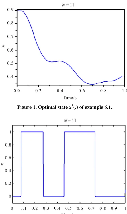
Example 6.1 We first consider a problem containing non-smooth function H t u t



,

 



which indirect approa- ches (base upon pontryagin maximum principle) can not dealing with this case in a proper way. The problem is to find the control u t

 

and the state x t

 

which mini-

mize

 





 

1 0

= sin 2π e t d

J



t   x t t (6.1)

subject to

 

₌



5 2



 

 

3_esin 2 πt

x t t  t t x t u t (6.2)

with u t

 

 



1,1



, x

 

0 = 0.9 and x

 

1 = 0.4. Here

 





 

3 _{sin 2} _π

, = e t

H t u t u t , and according to the (4.2)

and (4.3) we have

 





 









sin 2 π

= min , : 1,1 = e t

u

g t H t u t u   and

 

= maxu





,

 



:



1,1 = 0





w t H t u t u  , thus

 

₌

 

 

_{= e}sin 2 πt_.

t w t g t

  In Figures 1 and 2 we plot

the optimized state x t

 

and control u t

 

for N = 11.

Also, the numerical results compared with the colloca- tion method [12] are listed in Table 1. From Table 1. one can see that our method achieves good result with a relatively smaller of nodes than [12].

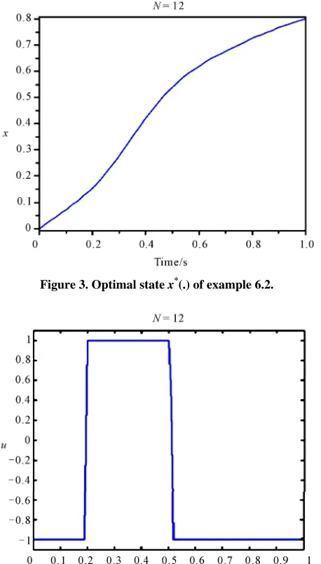
Example 6.2 Find the control u t

 

and the state

 

x t , which minimize





 

1 0 1

= e 2 d

2

t

J



  t x t t (6.3)

subject to

 

=

 

ln



 

3



x t tx t  u t  t (6.4)

with u t

 

 



1,1



, x

 

0 = 0 and x

 

1 = 0.8. Here

 



,



= ln



 

3



H t u t u t  t , and according to the (4.2)

[image:4.595.310.533.78.454.2]

and (4.3) we have

[image:4.595.314.534.82.254.2]

Figure 1. Optimal state x*(.) of example 6.1.

[image:4.595.308.539.506.590.2]

Figure 2. Optimal control u*(.) of example 6.1.

Table 1. Comparison of J* between methods.

N Legendre Method Collocation Method [12]

6 −0.0331943700 −0.0354240398

8 −0.0346216260 −0.0356414811

10 −0.0370224908 −0.0368552070

11 −0.0387730644 −0.0377178920

 

= minu





,

 



:



1,1 = ln







2



g t H t u t u  t and

 

= maxu





,

 



:



1,1 = ln







4



w t H t u t u  t , thus

 

=

 

 

= ln



4



ln



2 = ln



4

2

t

t w t g t t t

t

     



In Figures 3 and 4 we plot the optimized state x t

 

and

control u t

 

for N= 12. Also, the numerical results

[image:5.595.63.289.79.276.2]

Figure 3. Optimal state x*(.) of example 6.2.

[image:5.595.60.289.82.484.2]

Figure 4. Optimal control u*(.) of example 6.2.

Table 2. Comparison of J* between methods.

N Legendre Method Collocation Method [12]

7 −0.1820295698 −0.1815318828

9 −0.1825806940 −0.1821287778

11 −0.1826754624 −0.1823052407

12 −0.1828354838 −0.1826714837

index got by our approach are better than those obtained by the method in [12].

7. Conclusions

The aim of the present work is the determination of the

optimal control and state vectors by a direct method of solution based upon linear combination property of in-tervals and shifted Legendre series expansions together with the CGL points as collocation nodes respectively. The method is based upon reducing a nonlinear optimal control problem to an NLP. The unity of the weight function of orthogonality for shifted Legendre series and the simplicity of the discretization are merits that make the approach very attractive. Moreover, only a small number of shifted Legendre series is needed to obtain a very satisfactory solution. The given numerical examples supports this claim.

8. References

[1] R. R. Bless, D. H. Hoges and H. Seywald, “Finite Ele-ment Method for the Solution of State-Constrained Op-timal Control Problems,” Journal of Guidance, Control, and Dynamics, Vol. 18, No. 5, 1995, pp. 1036-1043.

doi:10.2514/3.21502

[2] R. Bulrisch and D. Kraft, “Computational Optimal Con-trol,” Birkhauser, Boston, 1994.

[3] G. Elnagar, M. A. Kazemi and M. Razzaghi, “The Pseu-dospectral Legendre Method for Discretizing Optimal Control Problems,” IEEE Transactions on Automatic Con- trol, Vol. 40, No. 10, 1995, pp. 1793-1796.

doi:10.1109/9.467672

[4] G. N. Elnagar and M. A. Kazemi, “Pseudospectral Che-byshev Optimal Control of Constrained Nonlinear Dy-namical Systems,” Computational Optimization and Ap-plications, Vol. 11, No. 2, 1998, pp. 195-217.

doi:10.1109/9.467672

[5] W. W. Hager, “Multiplier Methods for Nonlinear Optim-al Control Problems,” SIAM JournOptim-al on NumericOptim-al AnOptim-al, Vol. 27, No. 4, 1990, pp. 1061-1080.

doi:10.1137/0727063

[6] A. L. Herman and B. A. Conway, “Direct Trajectory Optimization Using Collocation Based on High-Order Gauss-Lobatoo Quadrature Rules,” Journal of Guidance, Control, and Dynamics, and Dynamics, Vol. 19, No. 3, 1996, pp. 592-599.doi:10.2514/3.21662

[7] M. Ross and F. Fahroo, “Legendre Pseudospectral Ap-proximations of Optimal Control Problems,” Lecture Notes in Control and Information Sciences, Vol. 295, No. 1, 2003, pp. 327-342.

[8] J. Vlassenbroeck and R. V. Dooren, “A Chebyshev Tech-nique for Solving Nonlinear Optimal Control Problems,” IEEE Transactions on Automatic Control, Vol. 33, No. 4, 1988, pp. 333-340. 10.1109/9.192187

[9] H. Seywald and R. R. Kumar, “Finite Difference Scheme for Automatic Costate Calculation,” Journal of Guidance, Control, and Dynamics, and Dynamics, Vol. 19, No. 1, 1996, pp. 231-239.doi:10.2514/3.21603

[image:5.595.60.283.545.636.2]

Solving Constrained Nonlinear Programming Problems,” Operations Research Annals, Vol. 5, No. 2, 1985, pp. 385-400.

[11] M. Razzaghi and G. Elnagar, “A Legendre Technique For Solving Time-Varing Linear Quadratic Optimal Control Problems,” Journal of the Franklin Institute, Vol. 330, No. 3, 1993, pp. 453-463.

doi:10.1016/0016-0032(93)90092-9