An invisibility cloak in a diffusive light scattering medium

light scattering medium

R. P. de Ruiter

light scattering medium

R.P. de Ruiter

Bachelor of Science thesis

January 2015

University of Twente

Faculty of Science and Technology

Complex Photonic Systems

Supervisors:

Abstract

Hiding objects with an invisibility cloak appeals to the imagination and also has many practical applications, such as to hide unwanted objects, to improve stealth techniques and to extend the range of wireless devices. An invisibility cloak can make it seem as if an object is not there by guiding light around it. Similarly, cloaks can hide objects from magnetism or heat.

In 2014 Schittny et al. presented an invisibility cloak based on the diffusion of light in a scattering medium. In such a medium light is scattered many times due to irregularities in the medium. Their cloak performed well for all wavelengths throughout the visible spectrum. In this research the cylindrical cloak of Schittny et al. is rebuilt and tested. Furthermore, methods to detect their cloak, i.e. breaking it, are discussed.

The design of Schittny et al. relies on the theory of the diffusion of light. This description of the behavior of light in a diffuse medium is extensively discussed and the requirements for perfect cloaking are derived analytically. The cloak consist of a cylinder with a shell placed in a background medium. Perfect cloaking is obtained by matching the diffusivities of the cloaking shell and the background medium. This result is confirmed by finite element simulations using COMSOL Multiphysics. For a homogeneous illumination, the perfect cloaking condition results in a uniform intensity behind the cloak for the 2D case in the absence of absorption in the system and for perfect diffuse reflection at the cylinder. For the 3D simulation the resulting intensity was not completely uniform, but this is possibly caused by the used mesh size and the finite height of the system.

In addition, physical experiments have been performed using a homemade cloak. The concentration of scatterers in the background medium was varied, leading to different diffu-sivities. The background medium was illuminated homogeneously on one side (inbound wall). The resulting intensity on the outbound wall of the container with the background medium was measured. A clear cloaking behavior was observed for diffusivities of the background that were close to the theoretical value for perfect cloaking. The intensity in the middle was still about 7% lower than the intensity of the background, probably caused by absorption of both the white paint on the cylinder as well as the shell itself.

The quality of the cloak was determined by comparing the resulting intensity profile of the cloak with that of an obstacle and an obstacle with a transparent shell. The cloak showed a more uniform resulting intensity than the obstacle for the expected perfect cloaking condition. An obstacle with a transparent shell lies in between in terms of quality.

Table of contents

1 Introduction 1

2 Theory 3

2.1 Mean free path and Beer-Lambert law . . . 3

2.2 Towards diffusion of light . . . 5

2.3 Requirements for perfect cloaking . . . 7

3 Simulations 11 3.1 Used model & boundary conditions . . . 11

3.2 Results . . . 13

4 Experiments 17 4.1 Setup . . . 17

4.2 Concentration TiO2in the background medium . . . 18

4.3 Influence of the position of the object on the intensity . . . 19

4.4 Different diffusivity ratios of the shell and the background medium . . . 20

5 Methods to break the cloak 25 5.1 Wavelength dependence of the diffusivity . . . 25

5.2 Refraction and reflection at the interface of the cloak and the background medium 29 6 Conclusion 31 7 References 33 A Radiative transport equation 35 A.1 Scattering and absorption . . . 35

A.2 Emission . . . 36

A.3 The equation of transfer . . . 37

1

Introduction

Invisibility is an intriguing phenomenon that frequently recurs in books, movies and circus acts. It is the ultimate way to escape from enemies or to hide unwanted objects. For that reason camouflage is widespread in nature and in military applications. However, camouflage works only if the observer looks at a certain angle to the object.

Guiding light around an object such that it seems as if the object is not there leads to angle independent invisibility and is called cloaking. In recent years the interest in cloaking has grown in science and there exist many cloaks nowadays, including cloaks for heat and magnetism [1, 2].

In artificial materials (so called metamaterials) the local optical properties can be tuned precisely. This makes it possible to guide light around an object without the occurrence of a shadow. An invisibility cloak based on metamaterials was made by Schurig et al. in 2006 and was operational in vacuum or air [3]. However, this only worked in a narrow frequency band. This is due to the fact that the light close to the cloak needs to exceed the vacuum light speed to be still in phase with the surrounding light, and only the phase velocity can be higher than the vacuum light speed in normal dispersive media [4–6]. The energy velocity is restricted by special relativity to the vacuum light speed.

To overcome this limitation, Schittny et al. presented an invisibility cloak based on the diffusion of light in a scattering medium in 2014 [5]. This cloak performed well for wavelengths throughout the visible spectrum. In such a scattering medium light is scattered many times due to inhomogeneities in the medium and thus the effective propagation speed is no longer close to the vacuum light speed. His team was able to make such a cloak by matching the diffusivities of the background medium and the shell (cloak) around the cylinder to be hidden. Even though this cloak seems to perform well, it is unlikely that it is unbreakable; in other words, impossible to detect.

In this research the cloak in a diffusive medium of Schittny et al. is recreated and tested. Limitations in applicability will be discussed as well as methods to detect the invisibility cloak. Also the approximations made by Schittny et al. will be studied and the requirements for a perfect cloak are derived.

Outline of this thesis

First of all in chapter 2 an overview of important parameters is given; the diffusion equation for light is derived, as well as the requirements for a perfect cloak. Subsequently, simulation results are presented for different diffusivities of the shell and the background medium and it is shown that the analytic solution for a perfect cloak indeed leads to cloaking behavior (chapter 3).

2

Theory

This chapter covers the theory needed to physically describe cloaking. First of all, the charac-teristic parameters for diffusive media are explained: the extinction, scattering and absorption cross sections and their corresponding mean free paths. Thereafter, the diffusion equation for light is derived from the radiative transport equation in section 2.2. Lastly, in section 2.3 the requirements for a perfect cloak are given for a cylinderical geometry.

2.1

Mean free path and Beer-Lambert law

Suppose light travels through an opaque medium, such as white paint, paper or fog. In such media, light rays are scattered many times due to random irregularities in the medium, also the cause of speckle patterns [7, 8]. A quantity of interest for such systems is the so called mean free path: the average distance that a photon travels before it is scattered or absorbed [9]. The expression for the scattering and absorption mean free path will be derived in this section, starting with the former.

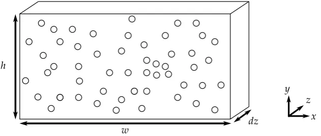
Imagine a container with scatterers that is illuminated in the z-direction. It is assumed that the scatterers are distributed homogeneously throughout the medium. The concentration of the scatterers isρ(particles/m3)and have a scattering cross section ofσsc(m2). This situation is depicted in Fig. 2.1. At a certain time a photon bounces off a scatterer. For simplicity,

dz w

h

y

x z

Figure 2.1: Infinitesimal thin slab of a container with many scatterers

assume that this scattering is elastic, the scattering cross-section is frequency-independent and that the scattering is isotropic: all outbound directions are equally likely and independent of the inbound direction. Then the probability that a photon collides with a scatterer in the interval dzis given by

P(collision) = Ascatterers

Atotal

= σscρwhdz

with Ascatterers the surface area covered by scatterers and Atotal the total surface area which is equal to the width w of the container times its height h. The decrease in ballistic (non-scattered) light intensity dT equals the incoming intensity T times the probability that the particle is scattered [8]

dT=−T(z)σscρdz (2.2) This is an ordinary differential equation with general solution

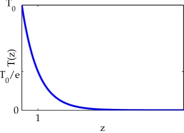
T(z) =T0exp(−σscρz) (2.3) This is the Beer-Lambert law for the ballistic light transport. The ballistic light intensity decays exponentially with position, scatterer concentration and the scattering cross section. In Fig. 2.2

T(z)versus thez-position is plotted forσscρ=1.

1 T 0 T 0/e 0 z T(z)

Figure 2.2: T(z)as function of z forσscρ=1

The probability that ballistic light is scattered in the interval dzis given by

dP(z) = T(z)−T(z+dz)

T0

=−1

T0

dT

dz dz (2.4)

The scattering mean free path l is the average distance that a photon travels between two succesive scattering events [9] and can be calculated now

lsc ≡ hzi= ∞

Z

0

zdP(z)

=− ∞ Z 0 z1 T0 dT

dzdz (Using Eq. 2.4)

= ∞

Z

0

zT(z) T0

σscρdz (Using Eq. 2.2)

= ∞

Z

0

zexp(−σscρz)σscρdz (Using Eq. 2.3)

= 1

σscρ (Integration by parts)

(2.5)

A similar relation for the absorption can be derived. In the case of only absorption and no scatterers present, the intensity distribution throughout the slab is given by

I(z) =I0exp(−σabρz) (2.6) withσabthe absorption cross section. With the absorption mean free path

lab= 1

σabρ (2.7)

The scattering and absorption cross sections can be combined to obtain the extinction cross section

σex=σsc+σab (2.8)

and the extinction mean free path

lex= 1

σexρ (2.9)

2.2

Towards diffusion of light

In the following section the way light propagates in a strongly scattering or diffusive medium is studied. For this purpose the time-independent diffusion equation for light is derived first.

To start with, the radiative transfer equation is taken (see for a derivation of this formula appendix A)

lexsˆ· ∇I(r, ˆs,ν) = a 4π

Z

p(cosΘ)I(r, ˆs0,ν)dˆs0−I(r, ˆs,ν) (2.10) with I(r, ˆs,ν) the spectral radiance, ˆsthe considered direction of propagation, ˆs0 a direction of propagation, ν the frequency of the light, p a phase function, a the ratio of the scattering and the extinction cross section andrthe position. See for a full definition of the parameters appendix A.

This equation is integrated over all angles to find the continuity equation [8]

∇ ·J(r) =−1−a

τ Id(r,ν) (2.11)

with Id(r,ν)the angular averaged diffuse intensity, which is related to the spectral radiance by

Id=

Z _dˆs

4πI(r, ˆs,ν) (2.12)

and the diffuse flux vector or photon current densityJ(r)[8, 10]

J(r) = lex τ

Z _dˆs

4πI(r, ˆs,ν) (2.13)

withτthe average time between two successive scattering events. If Eq. 2.10 is multiplied by ˆ

sand integrated

lex

Z _dˆs

4π(sˆ· ∇I(r, ˆs,ν))sˆ=a τ

lex

<cosΘ>J(r)− τ

lexJ

(r) (2.14)

since

Z _dˆs

4πdˆs

0_{p(sˆ, ˆs}0_{)I(r, ˆs,}

ν)ˆs=

Z Z

p(ˆs, ˆs0)ˆsdˆs0

1

4πI(r, ˆs,ν)dˆs

= τ

lex

<cosΘ>J(r)

If the system is strongly scattering, i.e. lex L with L the system’s size [11], then the angular distribution of the diffuse intensity is almost uniform [8]. Also it is assumed that the intensity is frequency independent. Therefore an approximation can be made [8]

I(r, ˆs,ν)≈Id(r,ν) +3τ

lexsˆ

·J(r) (2.16)

and Eq. 2.14 can be rewritten to [8]

τ

lex (1

−a<cosΘ>)J(r) =−lex

3 ∇Id(r) (2.17) The diffusion constant is defined by [8, 12]

D≡ 1

3

lex

τ

lex

1−a<cosΘ> = 1

3veltr (2.18)

and the transport mean free path by

ltr≡ 1

nσtr

= 1

n(σex−<cosΘ>σsc)

= lex

1−a<cosΘ> (2.19) Hence the diffuse flux vectorJ(r)equals

J(r) =−D∇Id(r) (2.20) The stationary diffusion equation is obtained by inserting Eq. 2.20 into the continuity equation Eq. 2.11

∇ ·(−D∇Id(r)) =− 1−a

τ Id(r) (2.21)

The light tends to go to regions with a higher diffusivity, just like heat tends to go to regions with a higher thermal conductivity and electric current to higher conductivity. If there is no absorptiona=1 (see Eq. A.9), then the divergence of the diffuse flux vector is zero

∇ ·J(r) =0 (2.22)

In this case, for each region whereDis constant,I(r)satisfies the Laplace equation

∇2Id(r) =0 (2.23)

which arises in many physics’ problems. The solutions to this equation are called harmonic functions.

The stationary diffusion equation (Eq. 2.21) is valid after the Thouless time after turning on a time continuous source [11]

ts= L

2

D (2.24)

with Lthe thickness of the diffusive medium. The Thouless time is the average time a photon spends in the diffusive medium [7]. For L = 60 mm and D = 1.75·104m2/s this gives

2.3

Requirements for perfect cloaking

The goal of this section is to obtain an expression for the different parameters to get a perfect cloaking behavior for a cylindrical object. That is, the light needs to scatter in a such way in the shell that it seems like there is no cylinder at all. To obtain the expressions for the parameters for a perfect cloak, Eq. 2.23 will be solved for this system and the right boundary conditions will be determined. In this derivation absorption is not considered. Instead of the intensity the photon densityn is used here. The equivalent to the diffuse flux vector is the photon current density and is [10]

j(r) =−D∇n(r) (2.25) The derivation is based on a similar derivation for electrical conduction by Milton [13].

2.3.1

Sketch of the situation

Suppose a cylindrical object needs to be cloaked. The cylinder has a radius R1with a perfect

diffusive reflection layer such that the diffusivity on the ledge of the cylinder is zero,D1=0.

It also ensures that no photons enter the cylinder.

This cylinder is placed in a medium with diffusivityD0. By applying a shell around this

cylinder with outer radiusR2it is possible to cloak this cylinder as shown in this section. This

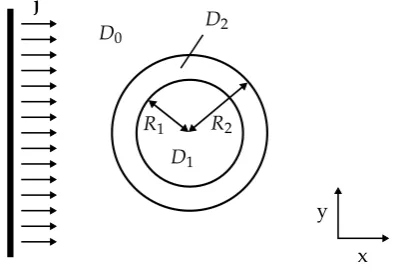
system is illuminated homogeneously in the forward x-direction. For a schematic view of this system, see figure 2.3.

D2

R2

R1

D1

D0

y

x

j

Figure 2.3: Schematic view of the system. The thick vertical line represents a light source that homo-geneously illuminates the cylinder in the forward x-direction as illustrated by diffuse flux vectorsj(r)

next to it

2.3.2

Photon densities in the different domains

First of all, a constant photon current density in the x-direction in the background medium for the aforementioned illumination is required, since it should look as if the light did not encountered any obstacles, i.e. j0 = a0xˆ. According to Eq. 2.20 the photon density in this

region is

n0(r) =a0x+b0 (2.26)

And because no light enters the core

n1(r) =0 (2.27)

natural. This part is based on a similar calculation for a spherical geometry by Griffiths [14]. In polar coordinates Laplace’s equation is given by

∇2_n= 1

r

∂ ∂r

r∂n

∂r

+ 1

r2

∂2n

∂θ2 =0 (2.28)

Using separation of variables gives solutions of the form

n(r) =R(r)Θ(θ) (2.29)

Inserting this into Eq. 2.28 gives

r R

∂ ∂r

r∂R

∂r

+ 1 Θ

∂2Θ

∂θ2 =0 (2.30)

The first term in this equation only depends on rand the second term only on θ. Therefore the individual terms should be constant

r R

∂ ∂r

r∂R

∂r

=k2 1

Θ ∂2Θ

∂θ2 =−k

2 _(2.31)

with k ∈ R. Instead of a partial differential equation (Eq. 2.28), two ordinary differential equations are left.

The general solution of the radial equation is

R(r) =Ark+Br−k (2.32)

And the for the angular equation it is

Θ(θ) =Csin(kθ) +Dcos(kθ) (2.33)

In the equations above A,B,C, andDare real-valued constants.

The photon densityn(r)should be continuous atr=R2, since the assumption is made that

there is no absorption. Eq. 2.26 carries a cos(θ)dependence only, soC=0. Thus the following separable solution for the photon density in the shell is left

n2(r) =

a2rk+b2r−k

cos(kθ) (2.34)

Here the constantDis absorbed into the constantsa2andb2.

The general solution for the photon density consists of the linear combination of the sepa-rable solutions.

n2(r) =

∞

∑

k=0

a2rk+b2r−k

cos(kθ) (2.35)

Since Eq. 2.26 is dependent on cos(θ), solutions up tok= 1 are taken and higher orders are neglected. Then, in summary, the photon densities in the three different domains are

n(r) =       

0 0≤r≤R1

a2+b2+ (a2r+b2/r)cosθ R1<r≤R2

a0rcosθ+b0 r>R2

(2.36)

2.3.3

Boundary conditions

The photon density should be continuous at the edges for all anglesθ, since the assumption is made that there is no absorption. For the edge between the shell and the background medium at cosθ=0 then

a2+b2=b0 (2.37)

This gives the following continuity equations for the photon density

0=a2+b2/R21, a0=a2+b2/R22 (2.38)

Also a continuity equation for the photon current density can be derived. From Gauss’s

theorem Z Z Z

V

(∇ ·j)dV =

Z Z

S

j·d~S=0 (2.39)

since∇ ·j=0 everywhere. Hence

Z Z

S

j·rˆdxdy=

Z Z

S

r(j·ˆr)drdθ=0 (2.40)

This equation is satisfied in all domains. At the edgesr=R1,R2the normal component of the

photon current density,j·rˆneeds to be continuous to ensure that the integral above is always zero, no matter how large the integration area is.

The normal component of the photon current density is given by

j·ˆr=−D∂n

∂r (2.41)

and can be evaluated using Eq. 2.36. This gives the continuity equations for the normal component of the photon current density on the edges

a2−b2/R21

D2=0,

a2−b2/R22

D2=a0D0 (2.42)

2.3.4

Condition for a perfect cloaking behavior

With all the above the condition for a perfect cloaking behavior can be obtained. Inserting eq. 2.38 into 2.42 gives (forD26=0)

a2= d2

R2₁, a2=−b2

D0+D2

R2₂(D0−D2) (2.43)

For a nontrivial solution (a2,b26=0)

R2₂ R2₁ =

D2+D0

D2−D0

→ D2

D0

= R

2 2+R21

R2₂−R2₁ (2.44)

3

Simulations

To show what happens for different ratios of the diffusivities of the shell and the background medium, as discussed in the previous chapter, finite element simulations have been performed using COMSOL Multiphysics. In this chapter those simulation results will be discussed. At first an overview of the model is given, including its boundary conditions.

3.1

Used model & boundary conditions

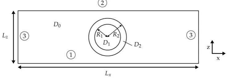
A simulation model was made for both a 2D and 3D system. The 2D model (or the top view of the 3D model) is depicted in Fig. 3.1. For the simulation model the system of Schittny et al. was taken as starting point, with Lx=355 mm,Lz =60 mm, 2R1=32.1 mm, 2R2 =39.8 mm,

D0=1.75·104m2/s, andD2=8.26·104m2/s. Perfect cloaking should occur forD2/D0=4.72

(see Eq. 2.44). The boundaries 1 and 2 are transparent walls in the physical setup, whereas the boundaries marked with 3 are black.

D2

R2

R1

D1

D0

z

x

Lz

Lx 1

2

3 3

Figure 3.1: Schematic view of the 2D simulation model or the top view of the 3D simulation. Figure is not drawn to scale

The 3D model is basically the 2D model with a height of Ly = 160 mm. For the top

y = 160 mm and bottomy =0 mm the same boundary condition as for the black walls 3 is taken. For the rest, the 3D model is identical.

As initial value Id = 0 was taken everywhere. Also dId/ dt = 0 was taken, since a time independent system is considered. On the boundary 1 the boundary condition

Id(r)−ze,1

∂Id(r)

∂z =−

a0ze,1

D at z=0 (3.1)

was taken as suggested by Bret [9], but now a source terma0 at the boundary is introduced.

from the surface and is [15]

ze,i= 2 3

1+R¯i

1−_R¯_iltr (3.2)

with ¯Ri the average reflectivity coefficient that can be calculated from Fresnel reflection coef-ficients and integrating over all angles [9]. The average reflectivity coefficient depends on the refraction indices of the media at the interface. A plot of the extrapolation length versus the average reflectivity coefficient is shown in Fig. 3.2.

0 0.1 0.2 0.3

R_i z e

4/3 l_tr

2/3 l_tr

Figure 3.2: Extrapolation length as function of the average reflectivity coefficient

For the opposite boundary 2 a similar condition was taken, but this time without a source term.

Id(r) +ze,2∂I

(r)

∂z =0 at z=L (3.3)

The container of the background medium is made out of Plexiglas, also known as PMMA, with a refractive index of nPMMA = 1.4924 for a wavelength of λ = 500 nm as calculated from the experimental data from Kasarova et al. [16] using the Sellmeier dispersion formula†_.

The background medium Schittny et al. used was deionized water with a refractive index of

nH2O = 1.3345 atλ = 500 nm and at a temperature of 21.5

◦_{C as calculated from the data of}

Daimon and Masumura [17]. This gives a refractive index contrast of 1.1183 from Plexiglas to water and a contrast of 0.8942 from water to Plexiglas. According to Bertolotti [15], this leads to an average reflectivity coefficient of ¯R1=0.20 and ¯R2=0.02 respectively. The background

medium that Schittny used had a transport mean free path of 233µm. From here the extrapo-lation length can be calculated and isze,1=233µm at the source 1 andze,2=162µm at the outbound wall 2 .

For the black walls 3 the boundary condition

D∂Id

∂z =qId (3.4)

is taken, with q an absorption term that is chosen such that the derivative of the intensity resembles a negative delta peak at the black walls, i.e. qD/Id.

Since all light that is incident on the cylinder is scattered diffusely, the normal component of the photon current density should be zero on the edge of the cylinder (see also section 2.3)

−ˆr·(−D∇n) =−J·rˆ=0 (3.5)

3.2

Results

First of all the direction of the photon current density has been plotted for the 2D case for a theoretical perfect cloak and is shown in Fig. 3.3. The direction of the photon current density is the same before and after the shell, thus the light is succesfully guided around the cylinder. Note that the figure does not provide any information of the magnitude of the photon current density.

Figure 3.3: The direction of the diffuse flux vectorJ(r). The length of the arrows does not provide any information about its magnitude

The intensity on the outbound wall 2 for the 2D case is shown in Fig. 3.4 for different dif-fusivities of the shellD2. The used mesh size is chosen such that the results do not significantly

alter when making the mesh size even smaller. The intensity is normalized to the intensity of the background. Only the intensity profile of ±1/4·Lx from the center is considered, like Schittny et al. do to get rid of edge effects.

100 150 200 250

0.5 1 1.5

Intensity (arb. units)

Position (mm)

D₂ = 1.75⋅104 m2/s

D

2 = 8.26⋅10

4 _m2_/s

D₂ = 8.67⋅104 m2/s

D₂ = 17.5⋅104 m2/s

Figure 3.4: The intensity on the outbound wall for the 2D simulation for different diffusivities of the shell. Perfect cloaking should occur for D2=8.26·104m2/s

For the case thatD2 = D0 = 1.75·104m2/s there is effectively only an obstacle of width

This shadow is indeed strongly present. For the case ofD2=8.26·104m2/s perfect cloaking is

expected and a uniform intensity is also observed in the middle region. For a slight mismatch in diffusivities of the shell and the background medium,D2=1.05·8.26·104=8.67·104m2/s,

a small peak occurs in the center. Light travels faster trough the shell now and thus is the observed intensity at the center higher. This effect is even more pronounced for the case of

D2=10·D0=17.5·104m2/s.

Likewise, these simulations have been performed for the 3D case. The results of this are shown in Fig. 3.5. Only the region of±1/4·Lxand±1/4·Lzfrom the center of the outbound wall 2 was considered, representing a physical size of 355/2 x 160/2 mm. False coloring has been used for visibility reasons. Red represents regions with high intensity, whereas blue represents regions with low intensity. The used mesh size was limited by the amount of memory of the computer (4 GB).

(a) D2=1.75·104m2/s (b) D2=8.26·104m2/s

(c) D2=8.67·104m2/s (d) D2=17.5·104m2/s

Figure 3.5: The intensity (false color) on the outbound wall of the 3D simulations for different diffusiv-ities of the shell D2. The latter are indicated in the subcaptions. Blue represents low intensity, red high

intensity. The background medium has a diffusivity of D0=1.75·104m2/s

Again an obvious shadow is observable for D2 = 1.75·104m2/s. Also the

overcompen-sation in the case of D2 = 17.5·104m2/s is clearly visible. The intensity is again higher in

the center than that of the background. The resulting intensity for D2 = 8.26·104m2/s and

8.67·104m2/s are not easily distinguishable from each other.

100 150 200 250 0.5

1 1.5

Position (mm)

Intensity (arb. units)

D₂ = 1.75⋅104 m2/s

D₂ = 8.26⋅104 m2/s

D

2 = 8.67⋅10

4 _m2_/s

D

2 = 17.5⋅10

4 _m2_/s

Figure 3.6: Integrated intensity on the outbound wall for the 3D simulation for different diffusivities of the shell D2. The intensities have been normalized to the background intensity

For D2 = 1.75·104m2/s and 17.5·104m2/s the graph looks like the graph of the 2D

case (Fig. 3.4). However, the intensity looks more uniform for D2 =8.67·104m2/s than for

D2 =8.26·104m2/s for this graph. This is probably due to the finite size of the cylinder and

4

Experiments

In this chapter various experiments are presented that investigate what the influence is of the position of the object inside and the concentration of scatterers in the background medium on the resulting intensity. Next to this, the cause and magnitude of experimental errors is discussed. Also the used setup is presented, which was based on the setup of Schittny et al.

4.1

Setup

The used setup is depicted in Fig. 4.1. As scattering background medium tap water con-taining white paint particles (titaniumdioxide) is used. The background medium has a dif-fusivityD0. This background medium is inserted in a homemade tank with internal

dimen-sions LxxLyxLz =355 x 160 x 61.6 mm. The tank is made of Plexiglas and has a transparent front and rear wall of 355 x 160 mm. All other walls are black to prevent the occurrence of waveguide-effects. To illuminate the tank, a standard 24” LCD screen is used to which various colored illumination patterns can be written. On the other side a Allied Vision Stingray F145B CCD camera was used to measure the intensity from the back side of the tank. This side of the tank is called the outbound wall. An objective was placed in front of the camera. The background medium is continuously stirred using two magnetic stirrers at the bottom of the tank.

CCD

D0

D1

D2 _Objective

LCD

z0

x z

Figure 4.1: Used setup

higher effective reflection losses. The outer radius of the cylinder isR1=15.9 mm.

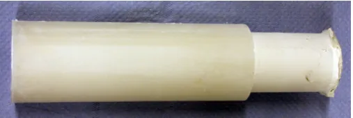
The cloaking shell is made of polydimethylsiloxane (PDMS) doped with melamine formalde-hyde (MF) resin micro particles with a diameter of d= 9.78µm with a standard deviation of 0.18 µm. Shells were made for 0 and 1.00 mg MF resin particles per mL PDMS. For this, the liquid PDMS was degassed using a vacuum desiccator before it was mixed with the micro particles and poured into a metal cast, leading to an outer radius of the shell of 14.5 mm. After mixing this suspension, curing agents were added at a ratio of 1:10 to start the polymerization of the PDMS. This process took about 4 hours at 80◦C. Hereafter, the mold was carefully re-moved. The cloak with 1.00 mg MF resin particles per mL PDMS is shown in Fig. 4.2. In reality the color of the cloak is less yellowish. Ideally, the cloak is completely white (no absorption). The cloak contained tiny bubbles, but they are not visible on the picture.

Figure 4.2: Cloak consisting of 1.00 mg MF resin particles per mL PDMS. In reality the cloak appears more white.

A typical measurement of the intensity on the outbound wall is presented in Fig. 4.3. In the figure false coloring has been using for visibility reasons, where red represents regions with high intensity and blue regions with low intensity. Only ±25 % from the center of the outbound wall is shown.

Figure 4.3: Typical measurement of the intensity (false color) on the outbound wall. Red respresents higher intensity, blue lower intensity. Only the±25% from the center of the outbound wall is shown.

According to Eq. 2.44 the ideal ratio of the diffusivity of the shell and the background medium for this system should beD2/D0=4.97, close to the value of the ratio for the system

of Schittny et al. of 4.72.

4.2

Concentration TiO

in the background medium

without shell). The background medium contained 2.0 g titaniumdioxide per mL water and was stirred manually every time in between the measurements. The resulting intensity as function of the x-position on the outbound wall of the tank (the wall closest to the CCD) was measured. The results of this are shown in Fig. 4.4. Here the intensity is integrated in the y-direction and normalized to the highest intensity. The 25% edge in the y-direction was removed before integrating. For the same concentration, it is expected that the intensity remains constant.

0

100

200

300

0.3

0.4

0.5

0.6

0.7

0.8

0.9

1

Position (mm)

Normalized integrated intensity

Figure 4.4: The integrated intensity in the y-direction as function of the x-position on the outbound wall for repetitive measurements where the background medium was manually stirred each time. The measurements were taken in the order from red to blue.

From the graph it is clear that the concentrations were not the same each time. The intensity of the background, the maximum of the intensity for the different measurements, ranges from 0.5 to 1.0. In the graph the order of the measurements is from red to blue. The intensity lowered every time after stirring. This can be due to that there was still paint on the bottom of the tank initially, and more and more was stirred upwards every time.

The standard deviation of the background intensity is σI = 0.17. Taking the standard deviation twice to obtain the 95% confidence interval for each measurement gives an error of ±0.34 in the intensity. Dividing this by the mean of the intensity of 0.72 the error in the concentration is obtained, since I ∝n−1 (see Eqs. 2.3 and 2.6). The error in the concentration is±0.47 g/L.

4.3

Influence of the position of the object on the intensity

Also the position of the obstacle was varied in the z-direction. From analytic results of Den Outer et al. [18] it is expected that there is a stronger shadow effect if the obstacle is closer to the wall nearest to the camera. Then the light has less time to diffuse into the region where the shadow appeared compared to a larger distance of the obstacle to this wall.

Fig. 4.1) are shifted such that the intensity is minimal atx =0. Only the central region of the intensity profile on the outbound wall is shown; the 25% border is removed before integrating. From the figure it becomes clear that there is indeed a more pronounced shadow effect for smaller distances from the center of the obstacle to the inner side of the outbound wall. The intensity profile is not completely symmetric, probably because the obstacle was not placed fully vertical, due to bumps at the bottom of the container.

−80 −60 −40 −20 0 20 40 60 80

0.5 0.6 0.7 0.8 0.9 1 1.1

Position from center (mm)

Normalized integrated intensity

z₀ = 24 mm

z₀ = 27 mm

z₀ = 29 mm

z₀ = 32 mm

z₀ = 36 mm

z₀ = 40 mm

Figure 4.5: The normalized intensity versus the position for various distances of the center of the obstacle to the inner side of the outbound wall z0(see Fig. 4.1 for a definition of z0). The intensity is integrated

over the y-direction and normalized to the intensity of the background. Only the central region of the intensity profile on the outbound wall is shown.

4.4

Different diffusivity ratios of the shell and the background

medium

For different concentrations of titaniumdioxide in the background medium the resulting in-tensity on the outbound wall was measured. This was done for an obstacle (no shell), a transparent shell (infinite diffusivity) and a cloak with a concentration of 1.00 mg MF resin per mL PDMS. For the latter, Schittny et al. found a diffusion constant ofD2=8.26·104m2/s for

particles with a diameter of dSchittny =10.2 µm. For isotropic scatteringltr =lexapplies (Eq. 2.19). The diffusivity is then proportional to the inverse of the concentration and the extinction cross section (Eq. 2.18): D∝(n·σex)−1.

The concentration in particles per mL PDMS isd3_Schittny/d3higher, but the geometrical cross section is onlyd2_/d2

Schittnywhich is approximately half the extinction cross section (see section

5.1). Correcting for the used particle size here, gives D2=7.92·104m2/s. The required value

of D0 for perfect cloaking for this system should be D0 = 1.59·104m2/s then, compared to

D0=1.75·104m2/s for the system of Schittny et al.

In Fig. 4.6 the results are shown for an obstacle. Again, only the region of±1/4·Lx and

pronounced shadow effect for higher diffusivities of the background medium. This makes sense, because the higher the diffusivity the more ballistic the response of the system is.

−80 −60 −40 −20 0 20 40 60 80

0.5 0.6 0.7 0.8 0.9 1 1.1

Position from center (mm)

Normalized integrated intensity

Obstacle

D₀ = 6.1⋅104 m2/s

D₀ = 3.0⋅104 m2/s

D₀ = 2.0⋅104 m2/s

D₀ = 1.7⋅104 m2/s

D₀ = 1.4⋅104 m2/s

Figure 4.6: The normalized intensity as function of the x-position on the outbound wall for an obstacle for different diffusivities of the background medium. The minimum of the intensity is shifted to x =0

for each curve. The intensity is integrated over the y-direction and normalized to the intensity of the background. Only the region of±25%from the center is shown.

The same measurement was repeated for the cloak as discussed above. The results are depicted in Fig. 4.7.

−80 −60 −40 −20 0 20 40 60 80

0.5 0.6 0.7 0.8 0.9 1 1.1

Position from center (mm)

Normalized integrated intensity

Cloaked obstacle

D₀ = 6.1⋅104 m2/s

D₀ = 3.0⋅104 m2/s

D₀ = 2.0⋅104 m2/s

D₀ = 1.7⋅104 m2/s

D₀ = 1.4⋅104 m2/s

Figure 4.7: The normalized intensity as function of the position on the outbound wall for a cloak for different diffusivities of the background medium. The cloak should work perfectly for D0 = 1.59·

104m2/s. The minimum of the intensity is shifted to x=0for each curve. The intensity is integrated over the y-direction and normalized to the intensity of the background. Only the region of±25%from the center is shown.

For diffusivities aroundD0 =1.59·104m2/s a uniform intensity of somewhat lower than

The cloaking behavior looks better for D0 = 1.4·104m2/s of the background instead of

1.59·104m2/s. But this is misleading. This has to do with the fact that the lower the diffusivity of the background the more time the light has to diffuse into the region where a shadow could appear. For very low diffusivities of the background medium, the intensity on the outbound wall will be pretty uniform, no matter what kind of obstacle is in the middle of the container as long as the obstacle is this small. Thus it is more fair to compare the cloak with the aforementioned obstacle at a fixed diffusivity of the background medium rather than looking at the cloak only. This comparison will be made later in this section.

Finally, the measurement was repeated for a cylinder with a transparent shell. The results hereof are shown in Fig. 4.8.

−80 −60 −40 −20 0 20 40 60 80

0.5 0.6 0.7 0.8 0.9 1 1.1

Position from center (mm)

Normalized integrated intensity

Obstacle with transparent shell

D₀ = 6.1⋅104 m2/s

D₀ = 3.0⋅104 m2/s

D₀ = 2.0⋅104 m2/s

D₀ = 1.7⋅104 m2/s

D₀ = 1.4⋅104 m2/s

Figure 4.8: The normalized intensity as function of the position on the outbound wall for a cylinder with a transparent shell for different diffusivities of the background medium. The minimum of the intensity is shifted to x=0for each curve. The intensity is integrated over the y-direction and normalized to the intensity of the background. Only the region of±25%from the center is shown.

Also here the lines are more flat than in the case of an obstacle (Fig. 4.6), but the well is deeper than with the use of a cloak. In the previous three graphs the intensity profile is not completely symmetric, probably because the different objects did not stand fully upright in the tank.

0

1

2

3

4

5

x 10

0.6

0.7

0.8

0.9

1

D

(m

/s)

Minimum of intensity

Cloak

Obstacle

Figure 4.9: The minimum intensity in the central region of the outbound wall for the cloak and the obstacle as function of the diffusivity of the background. The dotted red and blue lines are shown to guide the eye. The dashed black line shows the diffusivity of the background medium D0 = 1.59·104m2/s

for which perfect cloaking should occur.

From the graph a clear distinction between the cloak and the obstacle can be derived for diffusivities close toD0=1.59·104m2/s (dashed black line) for which a perfect cloaking

be-havior is expected. The cloak leads to a more uniform intensity profile than the obstacle does. For higher diffusivities of the background medium the minimal intensities are comparable for the cloak and obstacle (as discussed before). The cloak does not give a minimal intensity of 1 at D0=1.59·104m2/s, probably due to absorption of both the shell and the white paint that

5

Methods to break the cloak

Two methods to potentially break the cloak are discussed in this chapter. The wavelength dependence of the diffusivity will be discussed, as well as refraction at the interface of the shell and the background medium.

5.1

Wavelength dependence of the diffusivity

So far the diffusivity has been taken as a constant, that is, it is assumed that it is independent of the wavelength of the source. In this section this approximation will be discussed.

The diffusivity is proportional to the inverse of the extinction cross section for the case of isotropic scattering. Using Mie scattering calculations this cross section is calculated for different wavelengths. From here, the wavelength dependence on the diffusivity is calculated. To end with, the influence of the used wavelength on the ratio of the diffusivities of the shell and the background medium is calculated.

5.1.1

Background medium

The background medium consists of deionized water in the system of Schnitty et al. Using the experimental data of Daimon and Masumura [17] and fitting this to the Sellmeier equation an expressing for the refractive index as function of the wavelength can be obtained†

n2_H2O(λ) =1+ 5.689·10

−1_λ2

λ2−5.110·10−3+

1.720·10−1λ2 λ2−1.825·10−2+ 2.062·10−2λ2

λ2−2.624·10−2+

1.124·10−1λ2 λ2−1.068·10

(5.1)

See Fig. 5.1 for a plot of the refractive index as function of the wavelength.

400

1

500

600

700

1.5

2

2.5

3

λ

(nm)

n

H

O

TiO

2

PDMS

MF resin

Figure 5.1: Refractive indices of H2O, TiO2, PDMS and MF resin as function of the wavelength

In this background medium titaniumdioxide particles that act as scatterers are inserted and have a typical diameter of 200 nm [20]. In the approximation that the titaniumdioxide is isotropic the refractive index is equal to [20]

nTiO2 =

2no+ne

3 (5.2)

withnothe ordinary refraction index, which is given by [21]

n2o =5.913+

0.2441

λ2−0.0803 (5.3)

andnethe extraordinary refraction index given by [21]

n2e =7.197+

0.3322

λ2−0.0843 (5.4)

Here the imaginary part of the refractive index is neglected, since it is very small [22]. See again Fig. 5.1 for a plot of this function.

Using Mie scattering simulation software from Zijlstra [23], the scattering efficiency factor, the ratio between the scattering cross section and the geometrical cross section, i.e. Qsca =

400 450 500 550 600 650 700 1.8

2 2.2 2.4 2.6 2.8 3

λ (nm) Q sca

Background medium

Figure 5.2: The scattering efficiency factor for titaniumdioxide as function of the wavelength. The red line is a linear fit to the data.

The graph has a sinusoidal character. In the case of polydisperity (heterogeneous size distribution) the course of the graph will be smoothed [15]. This is probably the case for the household paint that Schittny et al. used. The red line is a linear fit to the data.

5.1.2

Cloak

The cloak is made of mono disperse MF resin particles with a diameter of 9.78 mm (standard deviation 0.18 mm). The refractive index for visible wavelengths of those particles is extrapo-lated from [24]. This MF resin particles are surrounded by PDMS with a refractive index that is highly dependent on the wavelength in the visible spectrum [25]. The refractive indices of those materials are shown in Fig. 5.1.

400 450 500 550 600 650 700 2.05

2.1 2.15 2.2

λ (nm)

Q sca

Shell

Figure 5.3: The scattering efficiency factor for the shell. The red line is a linear fit to the data.

As before, the graph has a sinusoidal character. Since the melamine is fairly monodisperse (homogeneous size distribution) there is less smoothing of the graph by means of different particle sizes, but still plays an important role [15].

5.1.3

Ratio of the diffusivities

The ratio of the diffusivities of shell and the background medium is the only thing that matters for a perfect cloak (see section 2.3). The diffusivity is proportional to the energy velocity and the inverse of the scattering efficiency factor. The energy velocity in both domains is given by the vacuum light speed divided by the refractive index of the most abundant material in the first approximation. That is in the background medium water and in the cloak domain the PDMS. The multiplication factor for the ratio of the diffusivities of the shell and the back-ground D2/D0is thus equal to the ratio(Qsca,0·n0)/(Qsca,2·n2). This ratio is plotted in Fig.

400 450 500 550 600 650 700 0.8

0.9 1 1.1 1.2 1.3 1.4

λ (nm)

(Q

sca,0

⋅

n 0

)/(Q

sca,2

⋅

n 2

)

Figure 5.4: The multiplication factor for the ratio of the diffusivities of the shell and the background as function of the wavelength.

Since polydispersity leads to averaging, a linear fit to the data has also been plotted. At 700 nm the ratio of D2/D0increased a factor 1.05. Gradually increasing the wavelength will

cause higher intensities at the center of the outbound wall, up to 3% for red light (Fig. 3.4). It is clear that the cloak no longer works perfectly. However, it remains questionable whether this is detectable with the used setup as discussed in chapter 4 due to experimental errors.

5.2

Refraction and reflection at the interface of the cloak and

the background medium

At the interface of the shell and the background medium there is refraction and reflection, since the refractive index of the shell (PDMS) differs from the background medium (water). Schittny et al. do not account for this. Light that is incident on the shell from the background medium will refract according to Snell’s law [26]

nisinθi=ntsinθt (5.5)

0

20

40

60

80

0

20

40

60

80

θ

(°)

θ

(°)

Figure 5.5: The angle of refraction as function of the angle of incidence for a water to PDMS transition (blue line). The black dashed line indicates the case when the incident and refracting medium have the same refractive index.

In the graph the blue line gives the angle of refraction as function of the angle of incidence for a water to PDMS transition. The black dashed line indicates the case when the incident and refracting medium have the same refractive index (no refraction). It is apparent from the graph that the light refracts towards the normal and thus more light tends to go effectively more towards the cylinder that should be hidden.

Also reflection occurs due to the mismatch in refractive index of the shell and the back-ground medium. The reflectivity from water to PDMS is 1% and is about 8% from PDMS to water [15].

6

Conclusion

The cloak of Schittny et al. has been recreated and tested. A cloaking behaviour was clearly observed in Fig. 4.7. However, the intensity in the middle region of the outbound wall of the container with the background medium was still about 7% lower than the intensity of the background, probably caused by absorption of both the white paint on the cylinder as well as the shell itself. The white paint on the cylinder could be replaced by making the cylinder itself out of a white material such as teflon.

Because the intensity becomes more and more uniform as the diffusivity of the background medium lowers, the intensity in the center using the cloak should be compared to the use of an obstacle. This is also studied and the results are depicted in Fig. 4.9. The cloak shows indeed a more uniform resulting intensity than the obstacle for the expected perfect cloaking condition. An obstacle with a transparent shell lies in between (Fig. 4.8).

The magnetic stirrers that were used at the bottom of the container were not powerful enough, so manual stirring was necessary. This lead to a large error in the concentration. The accurary of the measurements can be improved by using both stirrers at the top of the container and at the bottom. Also the bottom of the tank should be made completely flat such that the stirrers can spin faster without changing their position. The tiny bubbles in the cloak could be removed by placing the PDMS and the melamine for a longer time in a better vacuum.

In section 2.3 the condition for perfect cloaking was derived analytically. That this condi-tion works was subsequently demonstrated using simulacondi-tions in COMSOL Multiphysics. In the absence of absorption in the system and for perfect diffuse reflection at the cylinder, the condition results in a uniform intensity at the outbound wall. For 3D simulation the resulting intensity was not completely uniform, but this is possibly caused by the fact that the system is not infinitely high and/ or by the used mesh size.

One method to potentially break the cloak is making use of the fact that the ratio of the diffusivities of the shell and the background medium is wavelength dependent. This results in intensities up to 3% more in the middle region than intended for red light. By increasing the wavelength of the light of the source a peak in intensity in the centre should occur and the cloak could be, in theory, detected. This is however not measurable with the used experimental setup, because the relative error in the concentration of the background medium was 8.5%. In further research the absorption can be studied as well as the ratio of diffusivities outside the visible spectrum.

7

References

[1] R. Schittny et al., “Experiments on transformation thermodynamics: Molding the flow of heat,”Phys. Rev. Lett., vol. 110, no. 19, pp. 195901–195905, 2013.

[2] F. Gömöry et al., “Experimental realization of a magnetic cloak,”Science, vol. 335, no. 6075, pp. 1466–1468, 2012.

[3] D. Schurig et al., “Metamaterial electromagnetic cloak at microwave frequencies,”Science, vol. 314, no. 5801, pp. 977–980, 2006.

[4] D.A.B. Miller, “On perfect cloaking,”Optics Express, vol. 14, no. 25, pp. 12457–12466, 2006.

[5] R. Schittny et al., “Invisibility cloaking in a diffusive light scattering medium,” Science, vol. 345, no. 6195, pp. 427–429, 2014.

[6] E. Hecht,Optics, ch. 7, pp. 299–301. Pearson Education, Inc., 2002.

[7] E. Marakis, “Taming light propagation through strongly scattering media,” Master’s the-sis, University of Crete, 2014.

[8] P.N. den Outer,Multiple light scattering in random discrete media. PhD thesis, University of Amsterdam, 1995.

[9] B. Bret, Multiple Light scattering in porous gallium phosphide. PhD thesis, Van der Waals-Zeeman Instituut, 2005.

[10] R. Schittny et al., “Invisibility cloaking in a diffusive light scattering medium (supplemen-tary material),”Science, vol. 345, no. 6195, pp. 427–429, 2014.

[11] S.E.P. Faez, “Breakdown of diffusion approximation for light propagation in nano-porous gap sponges,” Master’s thesis, FOM Institute for Atomic and Molecular Physics, 2007.

[12] F. Van Beijnum, “Light takes no shortcuts - frequency dependence of the controlled prop-agation of light in random scattering materials,” Master’s thesis, University of Twente, 2009.

[13] G.W. Milton,The theory of composites, ch. 7, pp. 113–117. Cambridge University Press, 2002.

[14] D.J. Griffiths,Introduction to electrodynamics, ch. 3, pp. 137–139. Prentice-Hall, Inc., 1999.

[15] J. Bertolotti,Light transport beyond diffusion. PhD thesis, University of Florence, 2007.

[17] M. Daimon and A. Masumura, “Measurement of the refractive index of distilled water from the near-infrared region to the ultraviolet region,” Applied Optics, vol. 46, no. 18, pp. 3811–3820, 2007.

[18] P. N. den Outer , Th. M. Nieuwenhuizen, and A. Lagendijk, “Location of objects in multiple-scattering media,”J. Opt. Soc. Am. A, vol. 10, no. 6, pp. 1209–1218, 1993.

[19] P.P. Veugelers and B.M. Tel, “Algemene practicumhandleiding,” 2011. Handbook.

[20] L.E. McNeil and R.H French, “Multiple scattering from rutile TiO2 particles,”Acta

Mate-rialia, vol. 48, pp. 4571–4576, 2000.

[21] J.R. DeVore, “Refractive indices of rutile and sphalerite,” Journal of the Optical Society of America, vol. 41, no. 6, pp. 416–419, 1950.

[22] W.L. Vos et. al, “Broadband mean free path of diffuse light in polydisperse ensembles of scatterers for white light-emitting diode lighting,”Applied Optics, vol. 52, no. 12, pp. 2602– 2609, 2013.

[23] P. Zijlstra, “Mie-theory calculations using Matlab.” Internal report, 2005.

[24] H.B. Liu et al., “Optical properties of melamine formaldehyde resin,”Acta Physico-Chimica Sinica, vol. 16, no. 6, pp. 563–567, 2000.

[25] D.C. Miller et al., “Analysis of transmitted optical spectrum enabling accelerated testing of multijunction concentrating photovoltaic designs,”Optical Engineering, vol. 50, no. 1, pp. 013003–1–013003–17, 2011.

[26] F.L. Pedrotti et al.,Introduction to optics, ch. 2, pp. 16–22. Pearson Education, Inc., 2007.

[27] R. Elaloufi, R. Carminati, and J.-J. Greffet, “Time-dependent transport through scattering media: from radiative transfer to diffusion,”J. Opt. A: Pure Appl. Opt., vol. 4, pp. S103– S108, 2002.

[28] S. Chandrasekhar,Radiative transfer, ch. 1, pp. 1–10. Dover Publications Inc., 1960.

A

Radiative transport equation

The radiative transport equation describes how light propagates in a scattering, absorbing and emitting medium. In this appendix this equation will be derived for a stationary system. This derivation is based on [27–29].

A.1

Scattering and absorption

The most important parameter in radiative transfer theory is the spectral radiance I(r, ˆs,ν,t) or specific intensity as it is called in old literature [7]. Then the power P through a surface element dA in a solid angle dΩ around the direction ˆscan be described using this spectral radiance and is given by

dP=dI(r, ˆs,ν,t)cos(θ)dνdAdΩ (A.1)

for radiation within a frequency interval (ν,ν+dν) at a time t [27–29]. See Fig. A.1 for a situation sketch. In this relation θis the angle between sand the normal vector of dA. This construction is called apencil of radiation.

ˆ

s

dA

dΩ

θ

Figure A.1: Pencil of radiation

If radiation is propagating a distance dsin the direction of ˆs, radiation will be lost due to both scattering and absorption. At first, only scattering is considered. Analogously to Eq. 2.2, the radiation lost due to scattering can be described by

dI=−ρσscIds (A.2)

Therefore the radiation power is reduced by a rate of

or with dN=ρcos(θ)dAds

dP=−σscIdνdNdΩ (A.4) So far, the angular distribution the scattered radiation has not been considered. The question remains which fraction of radiation from another pencil of radiation ˆs0(θ0,φ0) = (sinθ0cosφ0, sinθ0sinφ0, cosθ0) is scattered into an element of solid angle dΩ0 at an angle of Θto the direction of incidence of the initial considered pencil of radiation ˆs. To do so, aphase

function p(cosΘ) =p(ˆs·sˆ0)can be introduced. The aforementioned fraction is then

dP=−σscIdνdNdΩp(cosΘ)dΩ

0

4π (A.5)

The rate of power loss in all directions is therefore

dP=−σscIdνdNdΩ

Z

p(cosΘ)dΩ

0

4π (A.6)

For the case of no absorption, the phase function should equal one

Z

p(cosΘ)dΩ

0

4π =1 (A.7)

If also absorption is taken into account, more power should be lost

Z

p(cosΘ)dΩ

0

4π =a≤1 (A.8)

It turns out that [29]

a= σsc

σex (A.9)

A.2

Emission

Until now only losses by means of scattering and absorption were studied, but emission was disregarded. An emission coefficientjcan be defined such that

dP=jdνdNdˆs (A.10)

gives the amount of radiant power originating from dN particles emitted into a solid angle element dΩfor light within a frequency interval (ν,ν+dν). The amount of radiation that is scattered from a pencil radiation in the direction of ˆs0 into a pencil radiation in the direction of ˆs0is according to Eq. A.5

dP=σscdNdνdΩp(cosΘ)Isinθ

0_d

θ0dφ0

4π (A.11)

Equating the previous two expressions gives the emission coefficient

j(θ,φ) = σsc 4π π Z 0 π Z −π

p(cosΘ)Isinθ0dθ0dφ0 (A.12)

The ratio between the extinction coefficient and the emission coefficient is called the source functionJ.

J= j

σex (A.13)

A.3

The equation of transfer

With all the above it is possible to derive the radiative transport equation. For this, imagine a small cylinder with a cross section dAand a height dsthrough which radiation within the frequency interval (ν,ν+dν) propagates in the direction of the normal of dA (θ = 0). The difference in radiant power between the two faces and confined to a solid angle dΩis

dI

dsdνdAdsdΩ (A.14)

This must come from the difference between the emitted radiation (Eq. A.10) and the radiation loss (Eq. A.3, including absorption this time)

jρdνdAdsdΩ−σexρIcos(θ)dνdAdΩ (A.15) Or

dI

ds =jn−σexnI (A.16)

Using Eq. A.13, this can be rewritten to

lexdI

ds =J−I (A.17)

or

lexsˆ· ∇I(r, ˆs,ν) = a 4π

Z

Acknowledgements

The work for this bachelor thesis has been carried out at the Complex Photonic Systems Group at the University of Twente. I would like to thank my daily supervisor Lyuba Amitonova for such good care, commitment to a succesfull conclusion, and for providing constructive feedback. And in particular I would like to thank her for helping me out with the simulation model in COMSOL. And also thanks to Sergei Sokolov for his assistance with the simulation model.

Besides I would like to specially thank Pepijn Pinkse, my supervising professor, for thinking along, his creative solutions, and for bringing me in touch with the right persons. From both supervisors I also greatly appreciate their flexibility, such that I was able to organize the Week of Inspiration, as well as the freedom I got to go my own way.

Next to them, it was without Andreas Schulz utterly impossible to develop the cloaks and this report had been very different, so a very heartfelt thank you to him. Also I would like to thank Allard Mosk, Devashish, Evangelis Marakis, and Maryna Meretska for the helpful discussions and for giving me new insights.

Last but not least I enjoyed the working atmosphere of the group incredibly. I was in good company of other inspiring and ambitious students and staff, which made the last phase of my Bachelor very enriching. For this I would like to express my gratitude to everyone. I had a wonderful time.

Rik de Ruiter