Adaptive Output Tracking for Nonlinear Network Control
Systems with Time-Delay
Jimin Yu, Haiyan Zeng
College of Automation, Chongqing University of Post and Telecommunications, Chongqing, China Email: [email protected], [email protected]
Received August 25, 2012; revised September 11, 2012; accepted September 17,2012
ABSTRACT
The problem of adaptive output tracking is researched for a class of nonlinear network control systems with parameter uncertainties and time-delay. In this paper, a new program is proposed to design a state-feedback controller for this sys-tem. For time-delay and parameter uncertainties problems in network control systems, applying the backstepping recur-sive method, and using Young inequality to process the time-delay term of the systems, a robust adaptive output track-ing controller is designed to achieve robust control over a class of nonlinear time-delay network control systems. Ac-cording to Lyapunov stability theory, Barbalat lemma and Gronwall inequality, it is proved that the designed state feedback controller not only guarantees the state of systems is uniformly bounded, but also ensures the tracking error of the systems converges to a small neighborhood of the origin. Finally, a simulation example for nonlinear network con-trol systems with parameter uncertainties and time-delay is given to illustrate the robust effectiveness of the designed state-feedback controller.
Keywords: Time-Delay; Network Control Systems; Backstepping Design; Adaptive Control; Output Tracking
1. Introduction
Network control system is a real-time closed-loop feed-back control system composed of sensors, controllers, actuators, etc. The advantages of network control sys-tems are its easy installation and maintenance, and its high reliability and flexibility [1,2]. In recent decades, there are lots of progresses in the study of stability of the network control systems [3-6].
However, in the closed-loop control of the network control system, the data transmission process is often produce time-delay. The time-delay of network control system often affects the stability and performance of the system, and may even cause the instability of the entire system [7]. Therefore, the impact of the time-delay on network control system needs to be considered when studying network control systems and designing control-lers. In [8], the authors analyzed the source of the time-delay of network control system. For the time-delay problem of network control system, a maximum allow-able delay bound satisfying the requirement of stability was proposed in [9], and the maximum delay caused by the network was estimated in [10]. For designing con-trollers of network control systems, in [11], the authors discussed a class of uncertain systems’ adaptive control scheme, and in [12] authors analysis robust stability of networked control systems with uncertainty. Although
some progresses are made in linear network control sys-tems, nonlinear network control systems with parameter uncertainties and time-delay needs to be studied. For example, in [13-17], the authors study the problems of adaptive robust control for uncertain systems and high- order uncertain nonlinear systems, and analyze the stabil-ity of the systems by Lyapunov stabilstabil-ity theory. But these papers did not consider the situation of the systems with time-delay.
2. Problem Description
In this paper, we consider a class of nonlinear network control systems with parameter uncertainties and time- delay, this system is described as
1
1
1
1
, , ,
,
1 1
, , ,
,
T
i i i i i
i i i
T
n n n n
n n n
x d t x u x x t
g x t h x t
i n
x d t x u u x t
g x t h x t
y x
(1)
where i
1, , i
1, ,
T i
x x x R i n , u R , and
y R are respectively the states, the control input and
system output, 1 is a vector of
un-known constant parameters, di(·) ≠ 0, ψi(·) and
, , T q
q R
ig
are unknown smooth functions, hi(0) = 0 (1 ≤ i ≤ n) is
also an unknown smooth functions, τis time-delay, and
τ≥ 0.
The objective of this paper is to design an adaptive feedback controller. The designed controller ensures the state of the closed-loop systems is bounded and the tra-jectory of output y(t) can asymptotic track reference sig-nal yr(t).
Assumption 1 For smooth function di(t, x, u), i = 1, ···,
n there exist functions : i i
c R R and : i 1
i
c R R
satisfies 0 < ci(x1, ···, xi) ≤di(t, x, u) ≤ci(x1, ···, xi + 1),
xn+1 = u.
Assumption 2 Because we have hi(0) = 0, then the
hi(x1(t)) can be expressed as hi(x1(t)) = γi(x1(t)), and
γi(x1(t)) satisfies the following assumption
1
1
i x t p x ti
where pi(x1(t)) is a known and smooth enough function.
Lemma 1 If the real number a≥ 0, b≥ 0, m≥ 1, then
there exist the following inequality
1
1
m m
a m
a b
m b
.
Proof for any real number x ≥ 0, y > 0, n > 0, by
Young inequality, we have
1 1
1
1 1
n n n n
xy x
n n
y .
Let a = x, 1
n b
n
y, m = n + 1 then we can release to Lemma 1.
Barbalat lemma [18] If x(t) is a uniformly continuous
function, and
0
lim t d
t
x exists and is bounded, then lim
0.tx
3. Adaptive Controller Design
In this section, by using the backstepping recursive method, we design a robust adaptive output tracking controller. The designed ideas of this method are de-scribed as follows: for the i-th equation of the system, constructed a suitable Lyapunov function, and designed virtual control law αi, the designed αi makes the
subsys-tem consist of previous i equations is stable, therefore, in step n, the designed controller u which makes the system consist of n equations stability is the true controller that makes the closed-loop control systems globally stable.
Step 1 Reference signal yr is a smooth function and
bounded, and its derivative r is also bounded, the
out-put tracking error is defined by ε1 = x1 – yr.
y
Constructed Lyapunov function as
2
1 1
1 1 1 d
2 2 2
t T
t
V q
x s s,where λ are positive, ˆ, ˆ is estimates of the unknown constant parameter θ. Calculating the deriva-tive of V1 along with system (1), we have
1 1 1
1 1 2 1 1 1 1 1 1
1 1
1 ˆ 1
2 ˆ
1 1 ˆ
2 T
T
r
T
V q x t q x t
d x g y h x t
q x t q x t
(2)
Because is bounded, presence non-negative smooth function r
y
,ˆw1 1 , satisfies
1 1 1 1
ˆT ,ˆ
r
g y w
.
By Lemma 1, for any real number σ that greater than zero, let a 1 w1
1,ˆ , b = σ, so that exists a smoothfunction 1
1,ˆ 0, satisfies
2
1w1 1,ˆ 1 1 1,ˆ
. (3) By using Young inequality, let constant ξ1 > 0 we have
12 2 2
1 1 1 1 2 1 1
1
1
2 2
h x t h x t
, (4)
select
2
1 1
2 1 1
q x t h x t
,
then we have
2
2
21 1 1 1 1
2 2
1 1
1 1
q x t h x t x t
, (5)
where ρ1(x1(t)) is a smooth function.
have
2
2 2
1 1 1 2 1 1 1 2 1 1 1
1
2 2 1
1 1
1 ˆ ,
2
1 ˆ
2
T
V d x x t
z
Designed virtual controller as
2 1
1 1
2 1 1 1
1 1
ˆ
2 ,
2
n c x
,
where 1(·) is smooth function that is greater than zero.
So that we can release to
2
1 1 1 1 2 1 1 2
2 2
1 1 1
2 1
1 ˆ
1 2
T
V n d x c z
n x t
1
And because –ε1α2≥ 0, by assumption 1, we have
2
1 1 1 1
2 2
1 1 1 1 1 2 2
2 1
1 ˆ
1 2
T
V n z
n x t c x
where η1 = 0.
Step 2 Let ε2 = x2 – α2, constructed Lyapunov function
as
2
2 1 2
1 1
d
2 2
t t
V V
q x s sCalculating the derivative of V2 along with system (1),
we have
2 1 2 2
2
1 1 1 1 1 2
2 2
1 1 1 2 2 3 2 2
2 1
2
2 1 2 1 1 1 1
1
2 2
2 2 2 1
1 2
1 ˆ
1
+ g
2
+ +g +
ˆ
+ ˆ +
1 +
2
T
T
T
T r
r
V V q x t q x t
n z c
n x t d x
d x h x t
x
y h x t
y
q x t q x t
Let
2
2 2 1
1
2 1 2 2
2
2 1 2
,
,
, ˆ
x
z z
Then we have
2
2 1 1 1 2 2 2 2 3
2 2
1 1 1 2 2 2
2 1
2 2
2 1 2 1 2
1
2
2 2 2 1 1
1
2 2 1
1 ˆ
+ g
2
+ +g ˆ
1 ˆ
1
+ .
2
T
T
r r
T
V n c x d x
n x t
d x z y
x y
z h x t
x
h x t q x t q x t
2
(6)
There exists a non-negative smooth function
2 1, ,2 ˆ
w , satisfies
2 2
2 2 1 2 1
1
2 1 2
ˆ
g +g ˆ
ˆ , ,
T T
r r
d x y z
x y
w
+ 2
2
By Lemma 1, let a2 w2
1, ,2 ˆ
, b = σ so thatthere exists a smooth function 2
1, ,2 ˆ
0, satisfies
2
ˆ
2 w2 1, ,2 ˆ 2 2 1, ,2
2
x
. (7) And because 1 x22 1 2 , combined with
Lemma 1, there exists a smooth function
2 1, ,2 ˆ 0
satisfies
2 2
1 1, 2 1 2 2 1 2 2 1, 2 ˆ
c x x x ,
. (8) By using Young inequality, let constant ξ2 > 0, μ2 > 0,we have
22 2 2
2 2 1 2 2 2 1
2 1
2 2
h x t h x t
2 2 2
2 2
2 1 1 2 2 1 1
1 2
1
2 2
h x t h x t
x
Select
2
2
2 1 1 1
2 2
2 2
1 1
q x t h x t h x t
2 2
2 1 1 1
2 2
2 2
2 2
2 2
1 2 1 1 1 1
2 2
2 2
1 1
1 1
q x t h x t h x t
x t x
t
Then we have
22 2 1 2 1 1
1
2 2
2 2
2
2 2 1 2 1
2
2
2
2 2
2
2 2 1 1 1
2
2
2
2 2
2
2 2 1 2 1
2 1 + ( ( )) 2 1 2 2 1 2 2 1 2 2
h x t h x t
x
q x t q x t
x t x t x t (9)
Substituting (7), (8), (9) into (6), we have
2
2 1 2 2
2 2 2
1 1 2 1 1
2 2
1 2
2
2 2
2
2 2 3 2 2 2 2
1 ˆ 1 2 1 1 2 2 + 2 T
V n z
n x t x t
d x
Designed virtual controller as
2 2
2 2
3 2 2 2
2 1 2
1
2 ,
n
c x x
where 2(·) is a smooth function that is greater than zero.
By assumption 1, we have
2 2
2 1 2 2 2
2 2
2
1 1 2 2 3
2 1 1 ˆ 1 2 1 2 T j j j
V n z
n x t c x 2
Step i After the recursive design step i-1, we can get a
group of smooth virtual controller as
1 1
2 1 1 2 2
1 1
, ,
, ,
, .
r
i i i i i i
y x
x x
where smooth function k(·) > 0, k = 1, ···, i – 1.
Constructed Lyapunov function as
2
1 2 1
1 1
d
2 2
t
i i i t
V V
q x s sThe derivative of Vi–1 as following
1 2
1 1 1
1 1 2 2 1 2 1 1 1 2 1 1 2 1 ˆ i
i j i i
j i j j j T i i
V n i c x
i n x t
z 1 i i
(10)Similar to step 2, we can prove (10) is also established in the step i.
Constructed Lyapunov function as
2 1 1 1 d 2 2 ti i i t
V V
q x s sIts derivative is given by
1 2 1 1 1 1 2 2 1 1 2 1 1 1 1 1 1 1 1 2 1 2 1 ˆ ˆ ˆ ii j i i i i
j i j j j T i i T
T i i
i i i i i r
r
i
T i
i j j j j j
j j
V n i c x
n x t
z
d x g y
y
d x g h x t
x
1 1 1 + . 2 i ii h x t
q x t q x t
Let 1 1 1 1 , , , ˆ i i
i i j
j j
i i i i
i
i i i
x z z
1 1 2
1 2 1 1 1 1 2 2 1 1 2 1 1 1 1 1 1 21 1 ˆ
2 1
ˆ
ˆ
i
i j i i i i
j
T i
j i i
j j
i i
i i i j j j
j j
T
T i T i
i i i r i i i
r
V n i c x
n x t
i d x d x g
x
g y z
y
z
1 1 1 1 1 + . 2 i ii i j
j j
h x t h x t
x q x t q x t
(11) There exists a non-negative smooth function wi(·),sat-isfies
1 1 1 1 ˆ ˆ iT i T
i i j j j i
j j
T
i i
r i i
r
g d x g
x
y z w
y i
By the Lemma 1, there exists a smooth function
βi(·) ≥ 0 satisfies
2
i wi i i
(12) Similar to step 2, there exists a smooth function
i
(·) ≥ 0 satisfies
1 2 2
1 1
1
i
i i i i j i i
j
c x
. (13)By using Young inequality, let constant ξi > 0, μi > 0,
we have
2 2 2
1 2 1
1
2 2
i
i i i i i
i
h x t h x t
2 1 2 1 1 1 2 1 2 1 1 2 1 2 i i ii j i
j j
i
j i
j i
i h x t
x
h x t
select
2
1 2
1 1
2 2
1
1 i 1
i j
j
i i
q x t h x t h x t
then we have
1 2 2 1 1 2 2 1 1 2 2 2 21 1 1 1
2 2 1 1 1 1 1 i i j j i i i i j j i i
q x t h x t h x t
x t x t
Then we have
1 1 1 1 2 2 2 1 2 2 21 2 1 2 1
1 2 2 2 2 1 1 2 1 + ( ( )) 2 1 2 2 1 1 2 2 1 2 2 i i
i i i j
j j i i i i i j j i i i i i i
h x t h x t
x
q x t q x t
i
x t x t
x t
Then we have
2 1 2 2 1 1 2 2 1 1 2 1 2 1 2 1 2 1 ˆ i ii j i i i
j
i
j
j j
T
i i i i i
V n i d x
n x t i
z i
Designed virtual controller as
2 1 1 1 2 , , i i ii i i i
i i
n i
c x x
where i(·) is a smooth function that is greater than zero.
By assumption 1, we have
2 2 2 1 1 2 1 1 1 1 1 1 2 1 ˆ . i ii j j
j j j
T
i i i i i i
V n i n x t
i c x z
Step n After repeated recurrence and proof, in the step
n, constructed Lyapunov function as
2 1
1 1 d
2 2
t
n n n t
V V
q x s s
2
1
2 2
1 1
2 1
1 1
1 ˆ
1 2
T n
n j n
j n
j
j j
n n n n
V n
n x t
c x
zn
(14)
From (14), we can obtain adaptive control law u and parameter ˆ following as
1
2
1 1
2 , , n
n
n n
n
n n
u
c x x n n
(15)
ˆ n
z
(16) where n(·) is a smooth function that is greater than zero.
Then, we have
2 21 1
2
1 1
1 2
n n
n j j
j j j
V n n x t 2
.
When n is large enough, then we have
2
1
n
n j
j
V n
Select 2 1
pn n j
j
, then we have
0
0
p dt
n n
V t V t
t n t . Therefore, we get 0 0
p d 0
.t
n t V t n t
By Barbalat lemma, we get , and then we have
lim pn 0
t
limtj 0
, j = 1, ···, n. So that we get
lim 0
t y t y tr .
So that the entire design procedure is reasonable.
Theorem 1 Considering closed-loop systems (1),
un-der assumption and Lemma, there exist a state feedback control law u and control law parameter ˆ. The closed- loop system is bounded for all allowable uncertainties and the output tracking error converges to a relatively small area, which satisfies
1 2 2
0Bt
r n
y t y t A B V e .
Proof
2
1
n
n j n
j
V n BV
A
where
min 2, 0
B
d . 2t t d
n
A n
q x s sBy Gronwall inequality, we have
0(0) .
Bt
n n
Bt n
V t A B V A B e
A B V e
And because
2 1
0 2
B t
j V tn A B Vn e
,
So that we have
1 2 2
0Bt
r n
y t y t A B V e .
In summary, for any real number ε0 > 0, in limited
time T > 0, the closed-loop system satisfies
r
0, 0y t y t t T .
4. Simulation Example
In order to show the effectiveness of the design scheme, we choose the nonlinear network control system with parameter uncertainties and time-delay as following:
1 2 1 1
2 1
1
T
x x x x t
x u x t
y x
(17)
In the simulation, for the closed-loop system (17), we choose the reference signal yr(t) = sint, time-delay τ =
0.01s, θ = 0.2, ξ1 = 1, ξ2 = 2, σ = 0.02, λ = 1, the initial
conditions x1(0) = 1, x2(0) = 0.5, ˆ(0) = 0.1, According
to (15) and (16), the control law u and the parameter of control law ˆ following as
2 2
2 2
2 2
2 2
1 1
1 2
2
2 2
1 2
1
2 2
1 1
4 4 2
ˆ 4
2 4
ˆ ˆ
ˆ 1
4
1
,
4 2
T r r
T T
r r
w
u x
x y
y x x
x x y
x y
2
2
1 1 2 1
1
1 1
2 2
1 1 2
2 1
1 ˆ
ˆ
( )
4
2 4
r
r
T r r
x x y x
x
x x y
x y
1
x y x x
x
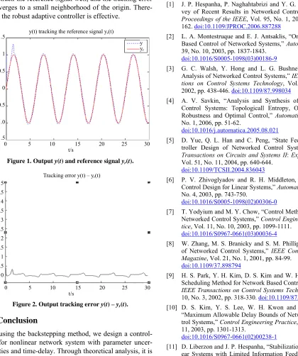
The simulation results are shown as in Figures 1 and 2.
It can be observed that the output of closed-loop system can track the reference signal well, and the tracking error converges to a small neighborhood of the origin. There-fore the robust adaptive controller is effective.
y(t) tracking the reference signal yr(t)
1.5
1
0.5
0
–0.5
–1.0
–1.5
0 5 10 15 20 25 30 t/s
y,
yr
[image:7.595.59.285.85.176.2]y yr
Figure 1. Output y(t) and reference signal yr(t).
Tracking error y(t) – yr(t)
0 5 10 15 20 25 30 t/s
5 4.5 4 3.5 3 2.5 2 1.5 1 0.5 0
y –
yr
Figure 2. Output tracking error y(t) – yr(t).
5. Conclusion
By using the backstepping method, we design a control-ler for nonlinear network system with parameter uncer-tainties and time-delay. Through theoretical analysis, it is shown that the designed robust adaptive output tracking
pressed the effectiveness of the scheme.
controller is feasible. The simulation results further
ex-6. Acknowledgements
part by the Natural Science
REFERENCES
[1] J. P. Hespanha Y. G. Xu, “A
Sur-This work was supported in
Foundation of Chongqing (CSTC) under Grant No. 2009BB3280, and the National Natural Science Founda-tion of China under Grant No. 60873200.
, P. Naghahtabrizi and
vey of Recent Results in Networked Control Systems,” Proceedings of the IEEE, Vol. 95, No. 1, 2007, pp. 138- 162. doi:10.1109/JPROC.2006.887288
[2] L. A. Montestruque and E. J. Antsaklis, “On the Model-
-9
Based Control of Networked Systems,” Automatica, Vol. 39, No. 10, 2003, pp. 1837-1843.
doi:10.1016/S0005-1098(03)00186
ushnell, “Stability [3] G. C. Walsh, Y. Hong and L. G. B
Analysis of Networked Control Systems,” IEEE Transac-tions on Control Systems Technology, Vol. 10, No. 3, 2002, pp. 438-446. doi:10.1109/87.998034
[4] A. V. Savkin, “Analysis and Synthesis of Networked
.2005.08.021
Control Systems: Topologicall Entropy, Observability, Robustness and Optimal Control,” Automatica, Vol. 41, No. 1, 2006, pp. 51-62.
doi:10.1016/j.automatica
te Feedback Con-[5] D. Yue, Q. L. Han and C. Peng, “Sta
troller Design of Networked Control Systems,” IEEE Transactions on Circuits and Systems II: Express Briefs, Vol. 51, No. 11, 2004, pp. 640-644.
doi:10.1109/TCSII.2004.836043
[6] P. V. Zhivoglyadov and R. H. Middleton, “Networked
2)00306-0
Control Design for Linear Systems,” Automatica, Vol. 39, No. 4, 2003, pp. 743-750.
doi:10.1016/S0005-1098(0
l Methodologies in [7] T. Yodyium and M. Y. Chow, “Contro
Networked Control Systems,” Control Engineering Prac-tice, Vol. 11, No. 10, 2003, pp. 1099-1111.
doi:10.1016/S0967-0661(03)00036-4
[8] W. Zhang, M. S. Branicky and S. M. Phillips, “Stability of Networked Control Systems,” IEEE Control Systems Magazine, Vol. 21, No. 1, 2001, pp. 84-99.
doi:10.1109/37.898794
[9] H. S. Park, Y. H. Kim, D. S. Kim and W. H. Kwon, “A Scheduling Method for Network Based Control Systems,” IEEE Transactions on Control Systems Technology, Vol. 10, No. 3, 2002, pp. 318-330. doi:10.1109/87.998012 [10] D. S. Kim, Y. S. Lee, W. H. Kwon and H. S. Park,
2)00238-1
“Maximum Allowable Delay Bounds of Networked Con-trol Systems,” Control Engineering Practice, Vol. 11, No. 11, 2003, pp. 1301-1313.
doi:10.1016/S0967-0661(0
ilization of
Nonlin-pp. 910-915. doi:10.1109/TAC.2005.849258 [11] D. Liberzon and J. P. Hespanha, “Stab
[image:7.595.73.493.212.714.2]Automatica [12] D. Yue, Q. Han and J. Lam, “Network-Based Robust
HControl of Systems with Uncertainty,” , Vol. 41, No. 6, 2005, pp. 999-1007.
doi:10.1016/j.automatica.2004.12.011 [13] L. Wei and R. Pongvuthithum, “N
Stabilization of Cascaded Systems withonsmooth Adaptive Nonlinear Param-eterization via Partial-State Feedback,” IEEE Transaction on Automatic Control, Vol. 48, No. 10, 2003, pp. 1809- 1816. doi:10.1109/TAC.2003.817932
[14] Z. Y. Sun and Y. G. Liu, “State-Feedback Adaptive Sta-bilizing Control Design for a Class of High-Order Non- linear Systems with Unknown Control Coefficients,” Journal of Systems Science and Complexity, Vol. 20, No. 10, 2007, pp. 350-361. doi:10.1007/s11424-007-9030-5 [15] Z. Y. Sun and Y. G. Liu, “Adaptive Stabilization for a
Large Class of High-Order Uncertain Nonlinear Sys-tems,” International Journal of Control, Vol. 82, No. 7,
2009, pp. 1275-1287. doi:10.1080/00207170802549529 [16] Z. Y. Sun, Y. G. Liu and Z. G. Liu, “An Adaptive
Con-troller for a Class of High-Order Nonlinear Systems with
rol for a Class of Nonlinear Systems,” 3rd
In-Control of Nonlinear Systems with Uncer-Unknown Control Coefficients,” Proceedings of the 30th Chinese Control Conference, Yantai, 22-24 July 2011, pp. 266-271.
[17] N. B. He, C. S. Jiang and Q. Gao, “Adaptive Backstep-ping Cont
ternational Conference on Measuring Technology and Mechatronics Automation, Shanghai, 6-7 January 2011, pp. 322-325.
[18] N. B. He, C. S. Jiang and Q. Gao, “Robust Adaptive Backstepping